Interactive parallel fluid solver using the Lattice-Boltzmann method and CUDA

(1)

INTERACTIVE PARALLEL FLUID SOLVER USING THE LATTICE-BOLTZMANN METHOD AND CUDA

Jorge Mario G. Mazo

EAFIT UNIVERSITY School of Engineering

Department of Informatics and Systems MEDELL´IN

(2)

INTERACTIVE PARALLEL FLUID SOLVER USING THE LATTICE-BOLTZMANN METHOD AND CUDA

Graduation project for the degree of: Computer Scientist

Assessor

Prof. Dr. Manuel Julio Garc´ıa

EAFIT UNIVERSITY School of Engineering

Department of Mechanical Engineering MEDELL´IN

(3)

“Well, it’s 1 a.m. Better go home and spend some quality time with the kids.” Homer Simpson

To my mother for all her support and patience during all these years. Also to my brother, my master and best friend. And to my sister, that although she is away, she has been closer than anyone else. They know that without them, this journey could not have been completed.

(4)

Abstract

Particle methods have been gaining momentum in the Computational Fluid Dynam-ics world, for their computational simplicity and inherent parallelism. This has lead the field to jump to new hardware technologies that exploit the parallelism in a whole new way.

This project is an interactive parallel implementation of the Lattice Boltzmann Method that runs on a hyper parallel architecture as a modern GPU and uses CUDA tech-nology for its implementation. First the mathematical concepts of the method are introduced, then the implementation is done using the SIMD paradigm, to later on attack the visualization and interactivity simple way.

(5)

Acknowledgements

There were many people involved on the development of this project and I would like to thank the following people: my advisor, Prof. Manuel J. Garcia, for returning me the faith in my degree. Also the fine crew of the Applied Mechanics Research Laboratory, Juan (abuelo) Duque, Santiago (kid) Orrego, Santiago (muerzo) Giraldo and Doriam for making the lab a fun place to work and learn. My friends Andres (chapa) Chaparro y Gustavo (tavo) Betancur, the university would have been such a boring place without those two guys.

Last but not least to my girlfriend Luisa (snake) Machado, grandma, all my aunts, my cousins and my nephew Juan Manuel, thank you all for your constant support.

(6)

3.3 Boundary conditions . . . 26 3.3.1 Periodic . . . 27 3.3.2 Bounce–back . . . 28 3.3.3 Von Neumann . . . 29 3.3.4 Dirichlet . . . 32 3.3.5 Corner nodes . . . 32 3.3.6 Moving boundary . . . 33 3.4 Units conversion . . . 34 3.4.1 Direct conversion . . . 35 3.4.2 Dimensionless conversion . . . 36 3.5 Algorithm summary . . . 37 4 CUDA implementation 38 4.1 Introduction . . . 38

4.2 GPUs as super computers. . . 39

4.3 Architecture of a GPU . . . 41

4.4 The need for speed. . . 41

4.5 CUDA . . . 42

4.5.1 Programming model . . . 42

4.5.2 Threads . . . 42

4.5.3 Memory layout . . . 44

4.6 LBM on the GPU . . . 46

5 Visualization and interactivity 49 5.1 Basic concepts . . . 49 5.1.1 Visualization . . . 49 5.1.2 Interactivity . . . 49 5.1.3 OpenGL . . . 50 5.2 Interactive tool . . . 52 v

(8)

5.2.1 Example. . . 52 5.2.2 Color scale . . . 53 5.2.3 Commands . . . 54 6 Numerical Experiments 56 6.1 Numerical results . . . 56 6.1.1 2–D Poiseuille flow . . . 56

6.1.2 Other common flows . . . 57

6.2 Computational results . . . 57

7 Conclusions 61 7.1 Future Work. . . 61

Bibliography 65 A Units Example 66 A.1 Channel case . . . 66

A.1.1 Initial approach . . . 67

A.1.2 Calculatingτ . . . 68

A.1.3 Different approach to calculateδt . . . 68

A.1.4 CalculatingN x . . . 68

(9)

List of Tables

1.1 Examples of correlation of properties with functionality and efficiency

of technical systems . . . 3

6.1 Poiseuille flow error committed by the solver . . . 58

6.2 Speed in MLUPs achieved by the GPU and CPU . . . 58

6.3 Speed in MLUPs achieved by different block sizes . . . 59

(10)

List of Figures

1.1 Numerical simulation procedure of engineering problems (Sch ¨afer). . 6

1.2 Mesh of an F–22 airplane(NASA). . . 7

1.3 Requirements and interdependences for the numerical simulation of practical engineering problems(Sch ¨afer).. . . 11

1.4 GPU performance improvements over CPU(RAMA HOETZLEIN).. . . 13

2.1 HPP lattice scheme . . . 15

2.2 HPP collision rules . . . 16

2.3 FHP hexagonal grid . . . 17

2.4 FHP collision probability . . . 18

2.5 FHP three particle head on collision rule . . . 19

3.1 LBM cartesian grid and vectors of the D2Q9 lattice.. . . 23

3.2 Two common lattice schemes for the Lattice Boltzmann Method . . . . 24

3.3 Vectors of the D2Q9 lattice. . . 24

3.4 LBM streaming step . . . 26

3.5 Stream step for a periodic boundary . . . 27

3.6 Pre–Stream step for a bounce–back boundary for a timet . . . 28

3.7 Post–Stream step for a bounce–back boundary for a timet . . . 29

3.8 Bounce–back of direction–specific densities . . . 29

3.9 Post–Stream step for a bounce–back boundary for a timet+dt . . . . 30

3.10 Post–Stream boundary node showing unknown direction–specific den-sities . . . 30

3.11 Corner node problem of boundary condition . . . 33

3.12 Post–Stream boundary node showing bounced direction–specific den-sities . . . 34

(11)

4.2 Design difference between GPUs and CPUs, taken from [NVI10] . . . 40

4.3 Memory bandwidth for the CPU and GPU, taken from [NVI10] . . . 40

4.4 Modern GPU architecture, taken from [KmWH10] . . . 41

4.5 Heterogenous programming model, taken from [NVI10] . . . 43

4.6 CUDA thread organization, taken from [NVI10] . . . 44

4.7 Transparent thread scalability, taken from [NVI10] . . . 45

4.8 CUDA memory hierarchy, taken from [KmWH10] . . . 46

4.9 LBM runs the same algorithm over each node of grid . . . 47

4.10 CUDA implementation in this work . . . 48

5.1 Simplified version of the Graphics Pipeline Process, taken from [wik10e] 51 5.2 Von Karman street . . . 52

5.3 Color saturation of a cavity flow, at the same timet . . . 53

5.4 Cavity flow pressure field . . . 54

5.5 MLUPS displayed . . . 54

6.1 Predicted velocity profile of Poiseuille flow . . . 57

6.2 Acceleration gained using GPU . . . 59

A.1 Sample Channel . . . 67

B.1 Point in polygon. . . 71

(12)

List of Algorithms

1 Lattice Boltzmann Algorithm. . . 37 2 Point inside the polygon . . . 71

(13)

Chapter 1

Introduction

The mankind nature to try to understand what it is around, has driven humans to study the environment we are immersed in... fluids. We are surrounded by fluids, water and air, and until recently we knew little about the behavior of those and the impact they have in our lives.

1.1

Mechanics of Fluids

Fluid mechanics is a filed that study the substances that continually flow under an applied shear stress and the forces on them. It can be divided into fluid statics, the study of fluids at rest, and fluid dynamics, the study of fluids in motion [wik10c]. Fluid dynamics, is an active field of research with many unsolved or partly solved problems. This makes the field, an interesting subject, to get involved in the scientific world.

1.1.1

Historical review

With only a rudimentary knowledge of fluid flow humans built wells, channels, pump-ing devices etc. With the exception of the works of Archimedes (287 – 212 B. C) on the principles of buoyancy, little knowledge of the ancient times is present on modern fluid mechanics. After the fall of the Roman Empire there is no record of advances in fluid mechanics until Leonardo da Vinci (1425–1519). He unleashed a new era in hydraulic engineering, he studied the flow of turbulent currents, the flight of the birds and the forces involved, although his work was impressive it was more artistic than

(14)

1.1. MECHANICS OF FLUIDS CHAPTER 1. INTRODUCTION science.

After da Vinci hydraulics gained momentum with great scientific contributions from Galileo, Torriceli, Marioti, Pascal, Bernoulli, Euler and d’Alembert. All their works were magnificent but there was always discrepancies between the theory and the practice, this discrepancy lead to the born of two schools of thought that still ex-ist today, the mathematica field of fluid mechanics know as hydrodynamics and the practical filed known ashydraulics.

Near the middle of the 1800s Navier and Stokes succeeded modifying the general equations for ideal fluid motion to fit in the viscous fluid, narrowing breach between hydraulics and hydrodynamics. Towards the end of that century four advances were crucial to the development of the fluid mechanics science, and there were: (1)The-oretical and experimental work by Reynolds, (2)Dimensional analysis by Rayleigh, (3)Use of model by Froude, Reynolds et. al and (4)Experimental and theoretical progress in aeronautics by Lanchester, Lilienthal, kutta, Joukwsky, Betz and Prandtl. The most important contribution was made by Prandtl in 1904 when he introduced the boundary layer, linking the ideal and real fluid motion for fluids with small viscosity [SWV96]. This contribution by Prandtl laid the ground of modern fluid mechanics.

1.1.2

Navier–Stokes and the fluid motion

Fluid motion can be seen in many different forms, from simple flows such as laminar flows in a pipe, to very complex flows including high degrees of turbulence. Many flows have been analyzed experimentally, however nowadays for more complex fluid flows is more convenient to develop a numerical approach capable of simulating many different flows, not yet analyzed experimentally.

In the following sections of this chapter a review of the equation of fluid motion will be presented. A set ofclassical numerical methods, to solve such equation will be presented, to later on move to small introduction to the relatively new particle methods and its implementation in new parallel hardware architectures.

Fluid motion of an incompressible fluid is governed by the continuity equation

(15)

1.2. NUMERICAL METHODS CHAPTER 1. INTRODUCTION

and the Navier–Stokes equation.

ρ ∂u ∂t +u· ∇u =_−∇p+µ_∇2u+f (1.2)

whereρ is density, u is velocity, p is pressure and µis the kinematic viscosity. The Navier–Stokes equation is a non–linear second order partial differential equation with not known analytical solution except for a small number of simplified cases.

With the advent of computer technology there has been attempts to approximate the solution of the Navier–Stokes equation using numerical analysis to simulate fluid flows.

1.2

Numerical methods

The functionality or efficiency of a technical system is always determined by some properties. A deep knowledge of these properties is needed in order to properly modify or optimize these technical system. In engineering and particular to fluid mechanics, some of these properties are:

• flow velocities. • temperature. • pressure

• drag or lift forces

A list with few examples of these properties related to fluid mechanics is given in Table1.1.

Property Functionality

Aerodynamics of vehicles Fuel consumption Pressure drop in vacuum cleaners Sucking performance

Pollutants in exhaust Environmental burden

Table 1.1: Examples of correlation of properties with functionality and efficiency of technical systems

(16)

1.2. NUMERICAL METHODS CHAPTER 1. INTRODUCTION

For engineering, the study of these properties are important for the redevelop-ment and enhanceredevelop-ment of products or processes. The knowledge gained from the study of important variables of fluid motion can help engineers to:

• improve efficiency • improve of durability • reduce pollution • save raw material

• have a better understanding of a process

In the industrial world cost reduction might be the key term related to the list men-tioned above but for scientists some times is more important to have a better under-standing of the process subject of study.

The importance of numerical methods arises from checking the available ods to gain knowledge on the properties of complex systems. The list of these meth-ods is very limited and be expressed as follows:

• Theoretical methods.

• Experimental investigations. • Numerical simulations.

Theoretical methods: analytical consideration of the equations of complex problem is not usually viable, the equations governing realistic physical phenomena are so complex (usually non–linear partial differential equations) that they are not solvable analytically for most of realistic applications.

Experimental investigations: aim to to obtain the required system information by the experimental tests. In many cases this can be rather problematic: the measures of the object are too big or too small making difficult to measure variables, the process elapses for a very small fraction of time to takes very long time to end, object of study cannot be accessed (a galaxy), the experiment is too risky, and the most important aspect for the industry is that experiments are time consuming and expensive.

(17)

1.2. NUMERICAL METHODS CHAPTER 1. INTRODUCTION

Numerical simulations: in–between theoretical methods and experimentation, in recent years numerical simulation has become a well established scientific and industrial discipline. Here physical phenomena is studied by means of numeri-cal methods on computers. The advantages of these compared to experimen-tation are:

• Faster results at lower costs.

• Parameter variations on the computer are usually easy.

• More comprehensive information about variables of the system.

An important prerequisite for exploiting the usefulness of numerical simulations are of coursecomputers. The booming in the computer industry has for sure helped the take–off of the numerical simulations, but numerical simulations are not and will never be a full replacement for experimental investigations and in general experi-mental validation should be accomplished to verify the accuracy of the numerical simulation.

The development of numerical methods is nothing new, Gauß and Euler where already working on numerical methods but due to the large number of computations required to approximate an equation no real benefit was extracted until the computer era. All the advances in computers like faster processors each year, better memory schemes, etc. have helped the mankind to really exploit the numerical simulations, however it was not just only the development in computers that helped the field to succeed but mayor improvements in numerical algorithms and better measurement tools. One can see that improvements in numerical simulation in the future are going to be fantastic, emerging new technologies like hyper–parallel processors (GPUs just to mention one), and new fast adaptive numerical methods will allow us to simulate more complex systems than ever before.

Based on this assumption one can presume that the demand for specialist in numer-ical simulation will be increasing in the near future, therefore the need to train and research on these topics.

Many aspects are involved during a numerical simulation. One mayor problem that arises in numerical modeling is the continuous analysis – usually engineering problems are differential or integral equations derived from continuum mechanics – continuum solutions are not viable due the fact the computational resources are

(18)

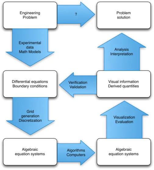
1.2. NUMERICAL METHODS CHAPTER 1. INTRODUCTION Engineering Problem Experimental data Math Models Differential equations Boundary conditions Algebraic equation systems Problem solution Grid generation Discretization Algorithms Computers Verification Validation Algebraic equation systems Visualization Evaluation Visual information Derived quantities Analysis Interpretation ?

Figure 1.1: Numerical simulation procedure of engineering problems (Sch ¨afer). limited and a discrete approach has to be taken. The unknown quantities have to ex-pressed by a finite number of values, this process is know asdiscretization [Sch06] and it has two main tasks:

• Discretization of the problem domain. • Discretization of the equations.

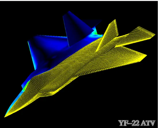
The discretization of a continuous problem consists in the division of the continuous domain in space and time into smaller sub–domains know aselements. The descrip-tion of a topology discretized by elements is know as mesh. Figure 1.2 shows the computer generated mesh of a war airplane.

(19)

1.2. NUMERICAL METHODS CHAPTER 1. INTRODUCTION

is because problems modeled with differential equations are expressed in terms of continuum variables in space and time.

There are several numerical techniques, to approximate the differential equations, and these are continuously improving due to the larger research in the area. Some of these techniques would be briefly reviewed in Section1.4.

An overview of setting up a numerical simulation can be seen on in Figure 1.1. Starting with an engineering problem that is described either by experimental data or differential equations and boundary conditions. This model is discretized into a set of algebraic equations suitable for solving with computers. The solution is accomplished by different techniques and the data is analyzed to obtain the problem solution.

(20)

1.3. COMPUTATIONAL FLUID DYNAMICS CHAPTER 1. INTRODUCTION

1.3

Computational Fluid Dynamics

Computational Fluid Dynamics or CFD is the analysis of systems involving fluid flow, heat transfer and associated phenomena such as chemical reactions by means of computer–based simulations[VM95]. The technique is very powerful and has a lot of industrial and scientific applications such as:

• aerodynamics • hydrodynamics • turbo–machinery • chemical process • meteorology • biomedical engineering

Since the 1960s the aerospace industry has been leading the way in the CFD arena integrating the methodology to the all its manufacturing chain. The CFD has lagged behind other numerical simulation techniques due to the tremendous com-plexity of the fluid flows. But the introduction of cheap high–performance computing solutions and easier programming models, leaded CFD to enter the industrial com-munity in the 1990s.

1.3.1

How does CFD works?

Pre–Processor

The pre–processor consist of the input of data parameters of a flow problem to a CFD program, this input is described in a form that the solver can understand. The activities at this stage include: meshing, setting fluid properties, choosing the solver and specifying boundary conditions.

Solver

The solver is where the numerical methods kick–in. After you have a model of a physical system, it’s necessary to compute the solution. Usually, the model is so

(21)

1.4. NUMERICAL METHODS FOR CFD CHAPTER 1. INTRODUCTION

large and complex that numerical methods are needed to approximate the solution, rather than attempting to get an “exact” solution.

Numerical solvers have a basic characteristics, and these have to efficient not just numerically but also computationally.

Many streams of numerical methods for CFD exist today, the classic approach using elements and the new trends usingparticles.

Post–processor

After the problem has been solved, the results are usually sets of data that cannot be easily interpreted by humans. The post–processor is a visualization tool that presents the output of the solver in such a way that can be easily interpreted and analyzed by people. Some of the possibilities that post–processors give, are: vector plots, particle tracers, viewing manipulations, etc. Also post–processing offers the possibility to operate the solver data into new variables of interest such as energy, vorticity, etc.

1.3.2

Problem solving with CFD

When solving fluid flow problems, we have to be aware that the physics are complex and that the solution is going to be at best as good as the physics and at worst as its operator. The user of CFD must have skills in a number of areas prior to set-ting up, running, and evaluaset-ting a solution. On CFD many assumptions have to be made according to the physics of the problem, and importation decisions regarding the modeling of the problem have to be taken. These decisions can determine the result of the problem, sometimes yielding improper results.

Also a good understanding about the numerical method is also crucial, key math-ematical concepts such as convergence, consistency and stability have to be always present for the CFD operator.

1.4

Numerical methods for CFD

Many methods have being created to study the fluid flows. The classical ones, the ones that have received more research and the trust of the industry are: the fi-nite difference method, fifi-nite elements method, spectral method and fifi-nite volume

(22)

1.4. NUMERICAL METHODS FOR CFD CHAPTER 1. INTRODUCTION

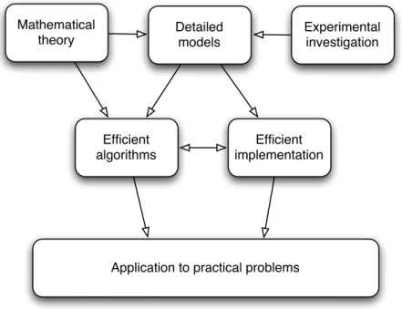
method. These methods will be explained in more detail below. Although they differ, the basic requirements for numerical simulations are the same for all methods, and these(requirements) are shown on Figure1.3.

1.4.1

Finite difference method (FD)

The FD methods describe the unknown function at the points of grid co–ordinate lines. Truncated Taylor series expansions are often used to generate finite difference approximations of the derivatives of the unknown functions in terms of point samples of the functions at each grid point and its immediate neighbors.

1.4.2

Finite elements method (FEM)

The FEM approximate solutions of partial differential equations (PDE) as well as of integral equations. The solution approach is based either on eliminating the dif-ferential equation completely (steady state problems), or rendering the PDE into an approximating system of ordinary differential equations, which are then numer-ically integrated using standard techniques such as Euler’s method, Runge-Kutta, etc[wik10b].

1.4.3

Spectral method (SM)

The SM approximate the unknowns by means of truncated Fourier series or series of Chebyshev polynomials. Unlike finite element method or the finite difference method the approximations are not local but valid throughout the entire computational do-main. The weighted residuals concept is also used to minimize the error similar to the finite element method.

1.4.4

Finite volume method

The FVM was originally developed as a special finite difference formulation. The method consists in three steps: the formal integration of governing equations over all the elements, converting the integral equations into a system of algebraic equations and then solving those system via an iterative method. The first step distinguishes the FVM from the other techniques because the resulting statements express the

(23)

1.5. PARTICLE METHODS “THE NEW TREND” CHAPTER 1. INTRODUCTION

exact conservation of relevant properties for each element[VM95].

In general all these methods involve the solution of large systems of linear equa-tions, making parallel computing practically a must for realistic applications.

Mathematical

theory Detailed models

Experimental investigation Efficient algorithms Efficient implementation

Application to practical problems

Figure 1.3: Requirements and interdependences for the numerical simulation of practical engineering problems(Sch ¨afer).

1.5

Particle methods “the new trend”

During the last few decades a new trend has been gaining popularity among the CFD community. This trend know as particle methods. Particle methods have be-come one of the most useful and widespread tools for approximating solutions of partial differential equations in a variety of fields. In these methods, a solution of a given equation is represented by a collection of particles, located in points xi and carrying masseswi. Equations of evolution in time are then written to describe the dynamics of the location of the particles and their weights.

Many particle methods exist, for example Smoothed Particle Hydrodynamics a mesh– free method, Molecular Dynamics, Lattice–Boltzmann, etc.

(24)

1.5. PARTICLE METHODS “THE NEW TREND” CHAPTER 1. INTRODUCTION

carrying physical information [eth10], this approach is deceivingly simple, yet power-ful and natural, method for exploring physical systems as diverse as planetary dark matter and proteins, unsteady separated flows, and plasmas.

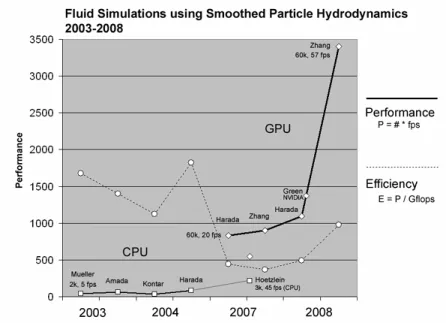
One big advantage of the Particle Methods is the inherent parallelism. This is due that in most cases each particle or packet of particles can be computed inde-pendently. This makes convenient the use of massively parallel architectures such as Graphic Processing Units (GPUs) to implement these numerical methods. The speed–up achieved but such architectures can be impressive in most application as shown in the Figure1.4. The figure shows how the raw power of GPUs has helped to get dramatical improvements in performance, but it also shows how the efficiency, has been dropping which means that hardware architectures are not been exploited to their fullest.

The Lattice Boltzmann Method was chosen for this work, because its highly par-allel capabilities, also the method uses a rectangular fixed grid, and Fix Grid FEM is a mayor area of research in the laboratory where this work is being done. This will allow future ideas of coupling between the two methods for the analysis of complex fluid–structure interactions.

This work presents a novel approach to interactive fluid simulations. A reliable and parallel–friendly method was necessary to achieve speeds fast enough to allow the user to interact with the simulation. The user would be able to move objects inside a fluid domain and it will get physically accurate feed back of different fluid variables as pressure, speeds and vorticity in almost real time, without the need of a post processing tool.

To get near real time speed a fast computing architecture is also needed, and most NVIDIA GPUs provide enough power, to supply the demanding needs of interactive simulations.

Finally, it has to be noted, that the arena of the parallel architectures is changing fast. The cell architecture (the one used by the Sony Play Station 3) is becoming every day more appealing for the implementation of scientific applications because of its high powered parallel processors and its low cost [KPP06].

(25)

1.5. PARTICLE METHODS “THE NEW TREND” CHAPTER 1. INTRODUCTION

Figure 1.4: GPU performance improvements over CPU(RAMA HOETZLEIN).

1.5.1

Document structure

The first part of the document is an introduction and theoretical view of the method subject of study. This first chapter was an introduction and presentation of the work realized in this project. Then on chapter 2, a review of the cellular automata is made as an introduction to the Lattice Boltzmann Method. Chapter 3 is a description of the Lattice Boltzmann Method and some others aspects particular to this project and the method itself.

The second part of the document consist in the computational aspects of the work, which are GPU computing and implementation of the method covered in chapter 4, and visualization and interactivity covered in chapter 5.

Finally the numerical results and benchmarks are described in chapter 6, and con-clusions and future work on chapter 7.

(26)

Chapter 2

Lattice gas automata

2.1

Background

A cellular automaton (CA) is a discrete model studied in mathematics, physics, mi-crostructure modeling and other sciences. It consists of a regular grid of finite cells, each one has a finite number of states, such as 1 and 0. For each cell, a set of cells (usually including the cell itself), known as neighborhood is defined relative to the specified cell.

An initial statet= 0is selected by assigning a state for each cell. A new generation is created after setting t = t+δt, according to some fixed rule, usually, a mathe-matical function [wik10a]. This determines the new state of each cell in terms of the current state of the cell and the states of the cells in its neighborhood.

2.2

Lattice gas automata

The lattice gas automata (LGA) also know as the lattice gas cellular automata (LGCA) is a cellular automata known as the precursor of the Lattice Boltzmann Method [Suc01]. Here with the purpose of introducing the Lattice Boltzmann Method is pre-sented a small review of the LGA methods.

The purpose of LGAs is to simulate the behavior and interaction of many single particles in an ideal gas [Vig09]. Unfortunately these are based on boolean mathe-matics which are unfamiliar for most people.

(27)

2.3. THE HPP MODEL CHAPTER 2. LATTICE GAS AUTOMATA

A cellular automata consist of a lattice geometry where the intersection points can take a finite number states. The model evolves in discrete time steps. The state of each corner is determined by its own state and the state of its neighbors at the previous time step. A gas is modeled as set of spheres that travel over the lattice. The collision between spheres is modeled by a set of elastic collision rules that ensure conservation of massm and momentum~p. The LGA, as molecular dynamics, works on a microscopic (lattice) level, but macroscopic quantities as densityρand velocityu

can be recovered from this level making possible the study of fluids at a macroscopic level.

2.3

The HPP model

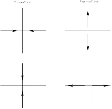
The HPP model was proposed by Hardy, Pomeau, and de Pazzisin in two landmark publications in 1973 [HPdP73a,HPdP73b]. In the HPP model the lattice is squared so each node has four neighbors. The particles can have four possible velocities determined bye_i = sin[π₂(i₋1)]i+ cos[π₂(i₋1)]j withi= 1..4as seen on figure2.1.

e2

e1 e3

e4

Figure 2.1: HPP lattice scheme

Each time step the particles are moved towards the ei direction. When two or more particles arrive to the same node during a time step a collision occurs. To meet the conservation of mass and momentum principles, the number of particles and the total velocity must be the same before and after the collision. When two particles collide they bounce into a direction perpendicular to their original direction as seen on figure 2.2. This preserves momentum as the sum of the velocities of the two particles is zero in both configurations. When three of four particles arrive to a same

(28)

2.3. THE HPP MODEL CHAPTER 2. LATTICE GAS AUTOMATA

P ost−collision P re−collision

Figure 2.2: HPP collision rules

node the only configuration that guarantees conservation of mass and momentum is the same configuration before the collision therefore the state is not changed (and cannot be changed). As a result in the method behaves as there was no collision. The collisions are deterministic, so each collision has one and only one possible re-sult. For this reason, this model has a property calledtime reversal invariance, that means that the model can be run in reverse to recover any earlier state.

The numerical density can be easily calculated, as the sum of all particle on a node at any given time.

ρ=X i

n_i (2.1)

Whereni is the boolean occupation number(0or1)expressing the number of parti-cles at a node with velocity ei. In this same way the velocity ucan be easily calcu-lated.

u= P

ieini

ρ (2.2)

(29)

2.4. THE FHP MODEL CHAPTER 2. LATTICE GAS AUTOMATA

2.3.1

Advantages and disadvantages

The HPP has some notable advantages and weakness. One big advantage is the boolean nature of the model, which makes its implementation using short ints ex-tremely fast.

Another advantage is the inherit parallel nature of the model, as each node can be computed independently only using the information of the particles.

Thetime reversal invariance feature is one of the greatest advantages as not many CFD models let you “travel” back in time.

Although this good advantages the HPP has one mayor flaw: it fails to achieve rotational invariance. This means that vortices using the method would look squared [Bui97], because of this the method was abandoned for simulation of fluid flows. Many other advantages and weaknesses exist in the method, but they are out of the scope of this review.

2.4

The FHP model

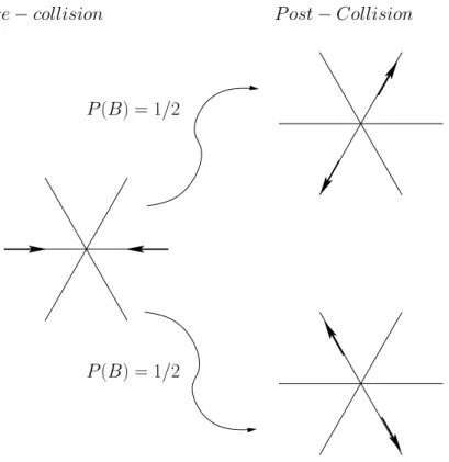
In 1986 Frisch, Hasslacher and Pomeau introduced the FHP model, moving from a square lattice to a hexagonal lattice, this added rotational invariance to the model which leads to the proper recovery of the Navier–Stokes equations[FHP86].

e6 e1 e2 e3 e4 e5

Figure 2.3: FHP hexagonal grid

The lattice velocity vectors are defined bye_i = cos[π₃ ₋π₆]i+ sin[π₃ ₋ π₆]j as shown in figure 2.3. The hexagonal grid allows that for a heads–on collision there is two

(30)

2.4. THE FHP MODEL CHAPTER 2. LATTICE GAS AUTOMATA

probable paths random chosen for the bounce as seen on figure2.4, this conserves mass and momentum in the same way as expressed in section2.3, but the introduc-tion of a probability makes the modelstochastic, this fact makes impossible thetime reversal invariance.

P ost₋Collision

P(B) = 1/2

P re₋collision

Figure 2.4: FHP collision probability

The FHP model also has a resolution for a three–particle collision this means that collision bounces back each particle back the way it came. This is shown in Figure 2.5, for all other collisions of four or more particles, no change should be computed[FHP86]. There are too many collisions allowed by this model, and the way to calculate can be found in [Bui97].

Many variations to the FHP model exist, these introduce new collision rules and resting particles. Interested readers should check into [Bui97] for a greater coverage of the different models of cellular automata.

(31)

2.4. THE FHP MODEL CHAPTER 2. LATTICE GAS AUTOMATA

P re

−

collision

P ost

−

Collision

Figure 2.5: FHP three particle head on collision rule

2.4.1

Advantages and disadvantages

The FHP model is essentially the HPP model with a change of the lattice geometry and extended collision rules set, therefore in inherits most of the advantages that HPP has.

Due to the stochastic nature of the model thetime reversal invariance is lost.

One big advantage over HPP is the introduction of the rotational invariance that per-mits to recover the incompressible Navier–Stokes equations.

One mayor disadvantage is the hexagonal mesh, such mesh elements are very computer–unfriendly[ST05], and hexagonal meshers are scarce, reason why the model did not take–off in the CFD world.

(32)

Chapter 3

Lattice Boltzmann Method

In 1998 McNamara and Zanetti proposed a fix to boolean nature of the Lattice Gas Automata[MZ88]. They removed the Boolean occupation numberni with an ensem-ble average

fi =hnii

sofi is a number between0and1. With this modification the evolution equation of a lattice gas automata became thelattice boltzmann evolution equation.

f(~x+~e, t+ 1)₋f(~x, t) = Ω(~x, t) (3.1)

McNamara and Zanetti proposed a way to simulate the ensemble average di-rectly in the numerical method instead of it being a theoretical quantity in an analytic derivation to prove the method’s conformance to the Navier–Stokes equation. The Equation3.1represents the main equation of study for the Lattice Boltzmann Meth-ods.

Since the method is no longer keeping track of single particles, it is are not longer in the microscopic scale. It has moved to amesoscopicscale, which means that one is now tracking averaged packets of particles.

It is mentioned here that from now on, vectors ~x, ~p and ~e are going to be just

(33)

3.1. BOLTZMANN EQUATION CHAPTER 3. LATTICE BOLTZMANN METHOD

3.1

Boltzmann equation

A familiar equation in the world ofstatistical mechanics the Boltzmann equation rep-resents the particle density in the position range x+dx and the momentum range

p+dp1at timet

f(x, p, t)dxdp

If there are no collisions, then at timet+dtthe position of particles starting atx

is going to be x+dx and the new momentum is going to be p+dp. This allows to calculate the momenta and positions of particles fort+dt if we know these values at timet:

f(x+dx, p+dp, t+dt)dxdp=f(x, p, t)dxdp (3.2) The Equation 3.2 is know in the Lattice Boltzmann Method world as the streaming step.

However there are collisions that result in particles at (x, p) not arriving at (x+

dx, p+dp)and particles that arriving at(x+dx, p+dp)but did not come from(x, p). It is setΓ−dxdpdtequal to the number of molecules that do not arrive to the expected phase space due to collisions during timedt. In the same wayΓ+dxdpdtis set to the number of particles that start somewhere different to(x, p)and end at(x+dx, p+dp). If this notion is added to equation3.2the following term is obtained:

f(x+dx, p+dp, t+dt)dxdp=f(x, p, t)dxdp+ [Γ+₋Γ−]dxdpdt (3.3) The first order terms of a Taylor series expansion of the left hand side of the Equation 3.3give the Boltzmann equation:

u_{· ∇x}f+F _{· ∇p}f+ ∂f

∂t = Γ

+₋_Γ−

(3.4) Where_∇x is (_∂x∂ ,_∂xβ∂ , ...), ∇x is (_∂p∂,_∂pβ∂ , ...), F is an external force andf is the dis-tribution function. It is to note that although Equation3.4was derived using an ideal gas as reference it can be derived for an arbitrary chemical component [ST05].

In its complete form Equation 3.4is a nonlinear integral differential equation and

(34)

3.2. LBM FRAMEWORK CHAPTER 3. LATTICE BOLTZMANN METHOD

it is particularly complicated to solve. With the Lattice Botlzmann methods an ap-proximation to the Equation3.3 is found with the particle perspective. This solution contains thecollideandstreamnotions, central to the Lattice Boltzmann Method and avoid one to solve the rather complicated Equation3.4.

3.2

LBM framework

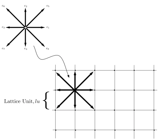
The lattice Boltzmann models simplify Boltzmann’s original concept by reducing the number of possible particle spatial positions and momenta from a continuum to a few possible results, and similarly the time is discretized totime steps. Particle positions are now confined to the nodes on the lattice, variations of momenta are reduced to8 directions and3 magnitudes, mass is reduced to a single particle mass. Figure 3.1 shows the cartesian lattice and velocitiesei wherea= 0, ...,8,e0 represents particles

at rest.

Not every lattice is appropriate for the Lattice Boltzmann Method. There are several conditions that have to be met to give the lattice sufficient isotropic behavior and allow a full recovery of the Navier–Stokes Equation [Suc01]. Some schemes have gained popularity due to easy implementation, some of these are shown in Figure3.2for the 2D and 3D cases.

Figure 3.3 shows the model known as the D2Q9. It is 2 dimensional (D2) and contains9velocities (Q9). This model has became the defacto standard for2D do-mains. Since this work comprehends a 2D domain the D2Q9 lattice was selected and it is used throughout this document. From now on when referring to a lattice, it is understood as the model mentioned above.

To comply with the isotropy condition, the 2DQ9 model must have the magnitude of the vector e_i and set of weights ω_i for each velocity. The velocity magnitude is given by ei =          0 for i= 0 1 for i= 1,2,3,4 √ 2 for i= 5,6,7,8

(35)

3.2. LBM FRAMEWORK CHAPTER 3. LATTICE BOLTZMANN METHOD

·

e0 e1 e2 e3 e4 e5 e6 e7 e8

{

Lattice Unit

, lu

Figure 3.1: LBM cartesian grid and vectors of the D2Q9 lattice. and the weights corresponding to the model implemented in this work are

ω_i =          4/9 fori= 0 1/9 fori= 1,2,3,4 1/36 fori= 5,6,7,8

3.2.1

Macroscopic variables

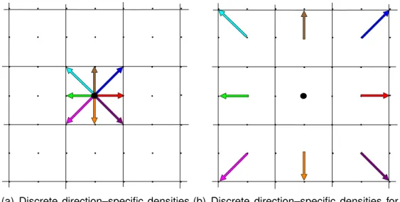
Since the method usesstatistical mechanics which is a great mathematical tool for dealing with large populations, of particles in this case, the frequencies can be con-sidered as direction specific fluid densities [ST05]. This the fluid density can be

(36)

3.2. LBM FRAMEWORK CHAPTER 3. LATTICE BOLTZMANN METHOD

(a) D2Q7 hexagonal lattice

28 Chapter 4 The lattice Boltzmann method

Table 4.2:Lattice vector bases and their weights for the D1Q3 and D3Q15 lattices. The complete set of vectors is all spatial permutations of the vectors given here.

(a) D1Q3 lattice Vector Weighting (0) t0= 2/3 (±1) ts= 1/6 (b) D3Q15 lattice Vector Weighting (0,0,0) t0= 2/9 (±1,0,0) ts= 1/9 (±1,±1,±1) tl= 1/72

Figure 4.2:The vectors of the D1Q3 lattice.

Figure 4.3:The vectors of the D3Q15 lattice.

(b) D3Q15 lattice

Figure 3.2: Two common lattice schemes for the Lattice Boltzmann Method

e0 e₁ e2 e3 e4 e5 e6 e7 e8

Figure 3.3: Vectors of the D2Q9 lattice. calculated using the following relationship:

ρ=

8

X i=0

fi (3.5)

and the macroscopic velocityu, is an average of the discrete velocitiese_i, weighted by the directional densities:

u= 1 ρ 8 X i=0 f_ie_i (3.6)

These two simple equation allows us to jump from the discrete microscopic velocities of the method to a continuum of macroscopic velocities that represent the fluid’s motion.

(37)

3.2. LBM FRAMEWORK CHAPTER 3. LATTICE BOLTZMANN METHOD

3.2.2

The equilibrium distribution function

The equilibrium distribution is used to simulate the collision between fluid particles. It can be derived from the Maxwell–Boltzmann velocity distribution from statistical mechanics: f_ieq(x) =ω_iρ(x) 1 + 3ei·u c2 + 9(ei·u)2 2c4 − 3u2 2c2 (3.7) It is proven that the equilibrium distribution of Equation 3.7 conserves mass and momentum [Vig09]. Equation 3.7is not the only equilibrium function available. This function can be modified to simulate different fluids like plasmas, non–newtonian fluids, etc.

3.2.3

The BGK model

So far the collision operatorΩ has not been discussed. The collision operator was proposed by Qian, d’Humieres, and Lallemand as a simplified collision operator sim-ilar to the one proposed for the Boltzmann equation by Bhatnagar, Gross, and Krook in 1954 [Vig09]. The BGK collision operator is given by

Ωi =−

1

τ [fi−f

eq

i ] (3.8)

whereτ is a free parameter known as the relaxation time, and f_ieq is the equilib-rium distribution function of particles. The collision operator represents the relaxation time of the distribution functionfi towards the equilibrium fieq. It is proven that this collision operator conserves mass and momentum [Suc01].

If we replace the BGK collision operator in Equation3.1the Lattice Boltzmann BGK model is obtained f_i(x+e_i, t+ 1) = 1₋ 1 τ f_i(x, t) + 1 τf eq i (x, t) (3.9)

It has to be mentioned that the value ofτ, – the time relaxation parameter –, cannot be chosen arbitrary because as τ _→ 0.5numerical instabilities arise in the method [ST05].

(38)

3.3. BOUNDARY CONDITIONS CHAPTER 3. LATTICE BOLTZMANN METHOD

·

(a) Discrete direction–specific densities for timet

·

(b) Discrete direction–specific densities for timet+dt

Figure 3.4: LBM streaming step

3.2.4

Streaming

In the streaming step, the direction–specific densities are moved one grid–node away in the direction they are pointing. This process can be seen on figure3.4.

3.2.5

Numerical kinematic viscosity

For the BGK D2Q9 model the numerical viscosity, which is not related to the physical viscosity, but to the relaxation parameter, is given by:

νlb = 1 3 τ ₋1 2 (3.10) Note that as mentioned on section 3.2.3 numerical instabilities arise when τ ap-proaches1/2. A value of τ = 1 is the safest [ST05] to keep the method numerical stable.

3.3

Boundary conditions

The Lattice Boltzmann Method has a rich set of boundary conditions, for many dif-ferent situations. All these boundary conditions vary in stability and convergence.

(39)

3.3. BOUNDARY CONDITIONS CHAPTER 3. LATTICE BOLTZMANN METHOD

In this work we are going to use periodic boundaries, bounce–back, and Zou/He for the flux and pressure boundary conditions. These boundary schemes are simple to implement and they are stable [LCM+08] in the range of the work comprehended here.

3.3.1

Periodic

With the periodic boundary conditions the system is closed by the edges and they are treated as they are attached to the the opposite edges of the domain. These boundaries as useful to simulate infinite domains, or finite repetitive (periodic) do-mains.

The boundary is easy implemented, the direction–specific densities pointing to out-side of the domain arestreamed to the corresponding directions in the other side of the domain as seen on Figure3.5.

·

(40)

3.3. BOUNDARY CONDITIONS CHAPTER 3. LATTICE BOLTZMANN METHOD

3.3.2

Bounce–back

As mentioned above the bounce–back boundaries are particularly simple and they have played a mayor role in making the Lattice Boltzmann Method popular for mod-eling complex geometries. The easiness of this boundary is that you just have to set a particular node as a solid boundary and nothing else has to be done. For ex-ample the a node marked with a 1 means that is a fluid and a node marked with a 0 is considered a solid boundary. No special treatment is necessary direction–wise or whatsoever. This makes the programming rather simple and makes the method suitable to complex geometries such as the found in porous media.

Here it is mentioned that many bounce–back schemes exists, but we are going to concentrate in the mid–plane full bounce–back. In this mode the solid wall (dark colored on the image) is between two lattice nodes as seen Figure3.6.

·

Figure 3.6: Pre–Stream step for a bounce–back boundary for a timet

After the direction–specific densities are streamed they are “absorbed” by they solid temporarily as outlined on Figure3.7. Then the direction–specific densities are reflected to the opposite direction. This process is shown in Figure 3.8. Finally in the next time step the direction–specific densities are streamed back into the fluid domain as seen in Figure3.9.

(41)

3.3. BOUNDARY CONDITIONS CHAPTER 3. LATTICE BOLTZMANN METHOD

·

Figure 3.7: Post–Stream step for a bounce–back boundary for a timet

·

Figure 3.8: Bounce–back of direction–specific densities

3.3.3

Von Neumann

Von Neumann or flux boundary conditions set the flow speed at a boundaries. A velocity vector (both components) are specified at the node from which density/pres-sure is computed.

Not just the density/pressure has to be computed, also unknown direction–specific densities appear at the boundaries and these have to be calculated properly to con-serve mass and momentum. Lets consider the inlet of a channel, at the first node on the east side, after the streaming step, some direction–specific densities are

(42)

un-3.3. BOUNDARY CONDITIONS CHAPTER 3. LATTICE BOLTZMANN METHOD

·

Figure 3.9: Post–Stream step for a bounce–back boundary for a timet+dt

known (shown dashed) as seen on Figure3.10.

·

Figure 3.10: Post–Stream boundary node showing unknown direction–specific den-sities

Using the know velocity set at the boundary and using Equations3.5,3.6and3.7 and assuming that direction–specific densities parallel to the boundary are equal to

(43)

3.3. BOUNDARY CONDITIONS CHAPTER 3. LATTICE BOLTZMANN METHOD

0, one can find the unknown direction–specific densities.

Let’s suppose that one want set a von Neumann boundary condition on the North lid. According to Figure 3.3, the direction–specific densities that have to be solved aref7, f4 andf8. The condition is a vertical velocity towards the south

u₀ = [0, v₀] (3.11)

Using Equation 3.6, one gets two equations, one for each component of the ve-locity vector

0 =f₁₋f₃+f₅₋f₆₋f₇ +f₈ (3.12) and

ρv0 =f2−f4+f5+f6 −f7−f8 (3.13)

As proposed by [ZH97], one can assume that the bounce–back is preserved in the direction normal to the boundary, so

f2−f2eq =f4 −f4eq (3.14)

This is a system of four equations and four unknowns, and it can be solved as follows. Equations3.5and 3.13have the unknown direction–specific densitiesf7, f4 and f8,

so they can be rewritten with those variables on the left hand side.

f4+f7 +f8 =ρ−f0−f1−f2 −f3−f5−f6 (3.15)

f₄+f₇ +f₈ =f₂+f₅+f₆₋ρv₀ (3.16) They the right hand sides are equated

ρ₋f₀₋f₁₋f₂₋f₃₋f₄₋f₅₋f₆ =f₂+f₅+f₆₋ρv₀ (3.17) and solve forρ

ρ= f0 +f1+f3+ 2(f2+f5+f6)

1 +v₀ (3.18)

Now, from Equation3.14one can solve forf4. As this equation contains the

(44)

3.3. BOUNDARY CONDITIONS CHAPTER 3. LATTICE BOLTZMANN METHOD

on Equation3.7, yielding

f4 =f2−

2

3ρv0 (3.19)

Substituting Equations3.12 and 3.19into the Equation 3.13 it can be solved for f7.

Equation3.19is used to replacef4 and Equation3.12is used to replacef8.

f7 =f5 +

1

2(f1−f3)− 1

6ρv0 (3.20)

to solve forf8, the last step can be repeated, except that Equation3.12is nows used

to substitute forf7 f8 =f6− 1 2(f1−f3)− 1 6ρv0 (3.21)

Now all the direction–specific densities are known, and the system configured properly to start a simulation.

3.3.4

Dirichlet

These boundary conditions constrain the pressure/density at the boundaries of the domain. The solution of these boundaries is very similar to the von Neumann ones. A density is specified at the node and with this information the speed is computed, and the remaining unknown direction–specific densities. Note that specifying density is equivalent to specifying pressure because they are related via an Equation of State of an ideal gas [Suc01]. For the D2Q9 the relationship is given by

p= ρ

3 (3.22)

The computation of the pressure boundary conditions, is very similar to the flux ones. Now instead of having a velocity, a density is specified at the node and the ve-locity vector is unknown. With this known density, the same process can be followed to solve for the unknown velocity and unknown direction–specific densities.

3.3.5

Corner nodes

With the model presented on Sections3.3.4and3.3.3serious problems arise at the corner nodes.

(45)

3.3. BOUNDARY CONDITIONS CHAPTER 3. LATTICE BOLTZMANN METHOD

·

(a) Pre–streaming of direction–specific densities

·

(b) Post–streaming of direction–specific densities

Figure 3.11: Corner node problem of boundary condition

direction–specific densities are known as seen on Figure 5.3(b), and we don’t have enough data to use Equations3.5,3.6and3.7to solve for the unknown densities.

Zou and He proposed a solution for this situation using the off–equilibrium den-sities. The idea is to bounce the know densities as seen on Figure 5.4. After the stream two densities are still unknown (show dashed), but now Equations 3.5, 3.6 and3.7can be used to find the two missing densities[ZH97].

It is quite obvious that these two densities after the streaming step do not aport any-thing to the fluid (they both are pointing towards outside the domain) but their value is needed to properly calculateρ, and this is going to be needed if we want o satisfy the conservation of mass.

This approach is different for velocity and pressure boundary conditions. It is fully developed for the pressure boundary conditions, for the velocity boundaries, some assumptions have to be made in order to retrieve all the values, this assumption introduces “noise”, that make the boundary prone to instabilities [ZH97].

3.3.6

Moving boundary

One of the novelty of this work is the ability to move objects inside the fluid inter-actively. Moving objects inside the fluid is a complex task since is prone to break the continuity of the model, this problem is solved by computing the new direction–

(46)

3.4. UNITS CONVERSION CHAPTER 3. LATTICE BOLTZMANN METHOD

·

Figure 3.12: Post–Stream boundary node showing bounced direction–specific den-sities

specific densities each time the object is moved. Also a new moment has to be computed, because the movement of the object adds a momentum to the particles towards the direction it is moved [Lad94].

f_i0 =fi−2ρ

wi(~ci·~u)

c2

s

(3.23) Where f_i0 are the bounced direction–specific densities fi, and ~u is the velocity of the moving obstacle inside the fluid. One key issue emerges of “when” to move the obstacle. In this work, the motion of the object is done based on the speed of the object. With this speed, it can be calculated the number of iterations needed to achieve onedx, and since this is a discrete system, the object will not be moved until all the iterations needed to move the object onedx have been calculated.

3.4

Units conversion

Lattice Boltzmann Method simulations represent the physics of actual macroscopic systems, but the method works at a microscopic level. This introduces the need to

(47)

3.4. UNITS CONVERSION CHAPTER 3. LATTICE BOLTZMANN METHOD

convert physical macroscopic units to microscopic units orlattice units.

There are two approaches to this conversion: the first one consist in converting from physical units straight to lattice units, and a more popular one that uses and intermediate dimensionless system to do the conversion.

There are several reasons why taking a intermediate step is preferred. Discrete vari-ables chosen, using this path, are directly related to important numerical parameters of the method, which have an impact on the accuracy and the stability of a simulation of the system [Lat08]. Also one may be in a situation in which there is no physical system to refer, like when you are benchmarking an article.

For these reasons more attention is going to be put into the second approach and a full developed example is shown in AppendixA.

3.4.1

Direct conversion

In this method the lattice units are related to physical units through the time step∆t

and the node spacing ∆x. The subscript is used to identify physical units is p and lb to identify Lattice Boltzmann Method units. The methodology described here is presented in Sukop and Thorne’s book [ST05].

The time step is given by the equation

∆t= νp

c2

s,p(τ −1/2)

(3.24) Whereν is the kinematic viscosity,cs,pis the speed of the sound, andτ the only free parameter is the relaxation time.

In the same way the space step is given by the equation:

∆x= νp

cs,lbcs,p(τ−1/2)

(3.25) The only missing parameter iscs,lb which can be found with the relation

cs,p =cs,lb

∆x

(48)

3.4. UNITS CONVERSION CHAPTER 3. LATTICE BOLTZMANN METHOD

The Equation3.26can be used to convert any desired speed from physical units to lattice units.

Similary for the pressure the resulting equation is

pp =p0,p

ρ_lb ρ0,lb

(3.27) Wherep0 is the reference pressure and ρ0,lb is the reference density. One can use the Equation3.22to relate the density and pressure to find the unknown parameters of this equation.

3.4.2

Dimensionless conversion

The dimensionless approach is described by L ¨att [Lat08]. In this approach a physical system is converted to a dimensionless system denoted by the subscriptd, and then converted lattice system. Taking dimensionless path is required for instance when analyzing lattice Boltzmann accuracy [Vig09].

For example one can use characteristic length l0 and time t0 and use them as a

base, to convert units to a dimensionless system. Take the physical timetp. This is given in a dimensionless notation by

td =

t_p t0,p

(3.28) and a lengthl can be described as

ld =

lp

l0,p

(3.29) In the same way, a unit conversion is introduced for other variables, based on a dimensional analysis. Take for example the physical velocityup:

up =

l0,p

t0,p

ud (3.30)

In the dimensionless system, the characteristic length and time of the system are both normalized to1. Then the dimensionless system is discretized into a grid

(49)

3.5. ALGORITHM SUMMARY CHAPTER 3. LATTICE BOLTZMANN METHOD

withN x nodes used to resolve its characteristic length. N iter time steps are used to resolve the system’s characteristic time. Space and time are then divided into intervalsδx andδtrespectively.

δx = 1

N x (3.31)

δt= 1

N iter (3.32)

And with this simple definition other variables, such as velocity and viscosity, are eas-ily converted between dimensionless system and lattice system through dimensional analysis: ud = δx δtulb (3.33) νd= δx2 δt νlb (3.34)

Although this a process looks complicated, it will be clarified by the example described on AppendixA.

3.5

Algorithm summary

A summary of the algorithm implemented in this work is presented here. One can notice the simplicity of the algorithm, which is one of the advantages of the method. Also it is noticeable, that for each time step the same algorithm is applied to each lattice node what makes the method fully data parallel and therefore convenient to a GPU implementation.

Algorithm 1Lattice Boltzmann Algorithm

while(TRUE)do

Calculate macroscopic variables: _→ρ=P8

i=0fi andu= _ρ1P8i=0fiei

Stream: _→f(~x+~e, t+ 1)₋f(~x, t) = Ω(~x, t)

Move obstacle: _→f_i0 =fi−2ρwi(~ci·~v)/c2s

Apply boundary conditions Collide: _→f_ieq(x) =ωiρ(x) h 1 + 3(ei_c2·u)+ 9(ei·u)2 2c4 −3u 2 2c2 i end while

(50)

Chapter 4

CUDA implementation

4.1

Introduction

Computers based on a single central processing unit (CPU), saw rapid performance increases and cost reductions for more than two decades. During this performance drive, software developers relied on advances on hardware technology to increase the speed of their applications. This trend, however, has slowed down since 2003, due to the power consumption and overheating issues of CPU cores[KmWH10]. Since then almost all CPUs have switched to multi–core models, where multiple pro-cessing units are placed onto a single chip to increase performance keeping power consumption and heat at a lower levels. This switch had a big impact on the soft-ware developer community due to the fact, that optimizations on performance where no longer handled by hardware, and had to be addressed by programmers during the coding of the software.

Traditionally software applications where written as sequential programs, these programs will only run on one of the processing cores, and will not achieve perfor-mance increases on modern multi–core CPUs. Now programs have to be written as parallel programs. Programs in which multiple threads of execution cooperate to achieve the functionality faster.

The parallel programming is nothing new. The scientific community has been developing parallel programs for decades. These programs run on large scale ex-pensive computers (clusters). Due to cost only few applications where allowed to run

(51)

4.2. GPUS AS SUPER COMPUTERS CHAPTER 4. CUDA IMPLEMENTATION

on those computers, making parallel software development rare and scarce.

4.2

GPUs as super computers

Since 2003 a kind of multi–core processors called Graphics Processing Units (GPU), have lead the race for computing performance. This performance gap is shown in Figure4.1 !"#$%&'()*(+,%'-./0%1-,! ! ! ! ! >17/'&()?)*( >@-#%1,7?6-1,%(A$&'#%1-,;($&'(B&0-,.(#,.( C&8-'D(E#,.F1.%"(G-'(%"&(!63(#,.(963( ! "#$!%$&'()!*$#+),!-#$!,+'.%$/&).0!+)!12(&-+)34/(+)-!.&/&*+2+-0!*$-5$$)!-#$!678!&),! -#$!978!+'!-#&-!-#$!978!+'!'/$.+&2+:$,!1(%!.(;/<-$4+)-$)'+=$>!#+3#20!/&%&22$2! .(;/<-&-+()!²!$?&.-20!5#&-!3%&/#+.'!%$),$%+)3!+'!&*(<-!²!&),!-#$%$1(%$!,$'+3)$,! '<.#!-#&-!;(%$!-%&)'+'-(%'!&%$!,$=(-$,!-(!,&-&!/%(.$''+)3!%&-#$%!-#&)!,&-&!.&.#+)3! &),!12(5!.()-%(2>!&'!'.#$;&-+.&220!+22<'-%&-$,!*0!@+3<%$!A4BC! !"#$% &'(% )$$#% &*(% +,-% )$$.% )$$/% )$$1% )$$0% )$$2% !"#/% !".$% 30$% 304% 32$% 35)% 36)$$% &*(% 9'-% !78% 9':% &*(% 9H2==(I(9&>-'0&(9HJ(2K=( 9L2(I(9&>-'0&(LK==(9HJ! 9K=!I!9&>-'0&!KK==!9HJ( 9M)!I!9&>-'0&!ML==!9HJ! 9M=!I!9&>-'0&!MK==!9HJ! N:O=!I!9&>-'0&!PK==!3@%'#! N:<Q!I!9&>-'0&!>J!QLQ=!3@%'#! N:<=!I!9&>-'0&!>J!QK==! #;$%3<=% >7-?)%@*7% #;)%3<=% <'-,?-A7B(% !"#$% !".$% 304% 32$% 32$% CDA-'% 32$% CDA-'% !7-AEB77F% G-?HI7AA%JJ% K77FI-?HA% <'-,?-A7B(%

Figure 4.1: Performance gap between GPUs and CPUs, taken from [NVI10] Such a large performance gap hasmotivated developers to move the computa-tionally intensive parts of a program to GPU for execution. These computacomputa-tionally intensive parts of the program is where the parallel programming focuses, because where more work is done, there is more chances of performance increases due to parallelization techniques.

The reason for such a large performance difference between the GPU and CPU, is that the GPU is specialized for compute–intensive, highly–parallel computations, exactly what graphics rendering is about, and therefore designed in such a way that more transistors are devoted to computing. In the other hand, CPUs are optimized for sequential code and I/O. For these reasons CPUs need more advanced control logic, and cache. This difference can be see on Figure4.2.

Not only the amounts in transistors makes a difference, memory bandwidth is also an important issue. GPUs have been operating at approximately 10x the bandwidth

(52)

4.2. GPUS AS SUPER COMPUTERS CHAPTER 4. CUDA IMPLEMENTATION! !"#$%&'()*(+,%'-./0%1-,! ! ! !234(5'-6'#771,6(8/1.&(9&':1-,(;*<! ! ;! ! !

=16/'&()>?*( @"&(852(3&A-%&:(B-'&(@'#,:1:%-':(%-(3#%#(

5'-0&::1,6(

! "#$%!&'%()*)(+,,-.!/0%!123!)&!%&'%()+,,-!4%,,5&6)/%7!/#!+77$%&&!'$#8,%9&!/0+/!(+:!8%! %;'$%&&%7!+&!7+/+5'+$+,,%,!(#9'6/+/)#:&!²!/0%!&+9%!'$#<$+9!)&!%;%(6/%7!#:!9+:-! 7+/+!%,%9%:/&!):!'+$+,,%,!²!4)/0!0)<0!+$)/09%/)(!):/%:&)/-!²!/0%!$+/)#!#*!+$)/09%/)(! #'%$+/)#:&!/#!9%9#$-!#'%$+/)#:&=!>%(+6&%!/0%!&+9%!'$#<$+9!)&!%;%(6/%7!*#$!%+(0! 7+/+!%,%9%:/.!/0%$%!)&!+!,#4%$!$%?6)$%9%:/!*#$!&#'0)&/)(+/%7!*,#4!(#:/$#,.!+:7! 8%(+6&%!)/!)&!%;%(6/%7!#:!9+:-!7+/+!%,%9%:/&!+:7!0+&!0)<0!+$)/09%/)(!):/%:&)/-.!/0%! 9%9#$-!+((%&&!,+/%:(-!(+:!8%!0)77%:!4)/0!(+,(6,+/)#:&!):&/%+7!#*!8)<!7+/+!(+(0%&=! @+/+5'+$+,,%,!'$#(%&&):<!9+'&!7+/+!%,%9%:/&!/#!'+$+,,%,!'$#(%&&):<!/0$%+7&=!"+:-! +'',)(+/)#:&!/0+/!'$#(%&&!,+$<%!7+/+!&%/&!(+:!6&%!+!7+/+5'+$+,,%,!'$#<$+99):<!9#7%,! /#!&'%%7!6'!/0%!(#9'6/+/)#:&=!A:!B@!$%:7%$):<.!,+$<%!&%/&!#*!');%,&!+:7!C%$/)(%&!+$%! 9+''%7!/#!'+$+,,%,!/0$%+7&=!D)9),+$,-.!)9+<%!+:7!9%7)+!'$#(%&&):<!+'',)(+/)#:&!&6(0! +&!'#&/5'$#(%&&):<!#*!$%:7%$%7!)9+<%&.!C)7%#!%:(#7):<!+:7!7%(#7):<.!)9+<%!&(+,):<.! &/%$%#!C)&)#:.!+:7!'+//%$:!$%(#<:)/)#:!(+:!9+'!)9+<%!8,#(E&!+:7!');%,&!/#!'+$+,,%,! '$#(%&&):<!/0$%+7&=!A:!*+(/.!9+:-!+,<#$)/09&!#6/&)7%!/0%!*)%,7!#*!)9+<%!$%:7%$):<! +:7!'$#(%&&):<!+$%!+((%,%$+/%7!8-!7+/+5'+$+,,%,!'$#(%&&):<.!*$#9!<%:%$+,!&)<:+,! '$#(%&&):<!#$!'0-&)(&!&)96,+/)#:!/#!(#9'6/+/)#:+,!*):+:(%!#$!(#9'6/+/)#:+,!8)#,#<-=!

)*?

!234

C(#(8&,&'#D>5/'$-:&(5#'#DD&D(

!-7$/%1,6(4'0"1%&0%/'&(

A:!F#C%98%$!GH

Interactive parallel fluid solver using the Lattice-Boltzmann method and CUDA