Q ingju Liu
Subm itted for th e Degree of Doctor of Philosophy
from the University of Surrey
UNIVERSITY OF
SURREY
C entre for Vision, Speech and Signal Processing Faculty of Engineering and Physical Sciences
U niversity of Surrey Guildford, Surrey GU2 7XH, U.K.
O ctober 2013
All rights reserved INFORMATION TO ALL USERS
The qu ality of this repro d u ctio n is d e p e n d e n t upon the q u ality of the copy subm itted. In the unlikely e v e n t that the a u th o r did not send a c o m p le te m anuscript and there are missing pages, these will be note d . Also, if m aterial had to be rem oved,
a n o te will in d ica te the deletion.
uest
ProQuest 27606655Published by ProQuest LLO (2019). C op yrig ht of the Dissertation is held by the Author. All rights reserved.
This work is protected against unauthorized copying under Title 17, United States C o d e M icroform Edition © ProQuest LLO.
ProQuest LLO.
789 East Eisenhower Parkway P.Q. Box 1346
Humans with normal hearing ability are generally skilful in listening selectively to a particular speech signal in the presence of competing sounds and background noise, such as a “cocktail party environment” . It is however an extremely challenging task to replicate such capabilities with machines. Bhnd source separation (BSS) is a promis ing technique for addressing this problem, which aims to recover the unknown source signals from their mixtures without or with little knowledge about the source signals and the mixing process. Among the existing BSS approaches, independent compo nent analysis (ICA) and time-frequency (TF) masking, are two popular choices for addressing the cocktail party problem, especially in a controlled environment, as these methods use few physically plausible assumptions about the sources and the mixing process. However, these algorithms are conducted mainly in the audio-domain, and their performance is limited by the acoustic distortions due to background noise and room reverberation, especially when such distortions become prominent. It is known th at both speech production and perception are bimodal processes, involving intrinsic interactions between audition and vision. For instance hp-reading helps the listener to better understand the target speech in a noisy and reverberant environment with multiple competing speakers. This thesis therefore considers the research question:
can the visual modality be useful for improving the performance of audio-domain B SS algorithms!
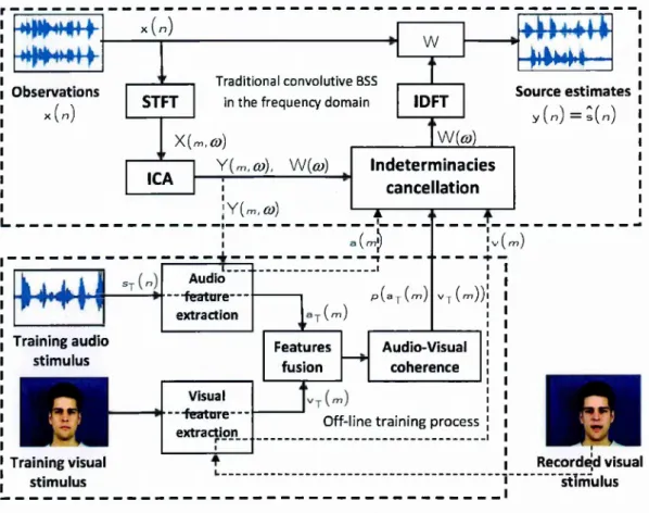
To this end, two key challenges have been studied in this thesis. Firstly, a proper evaluation of the audio-visual (AV) relationship, i.e. robust AV coherence modelling th a t takes into account the cross-modality differences in size, sampling rate and di- mensionahty. To address this problem, a global method with feature-based statistical characterisation, as well as a local method with sparse audio-visual dictionary learn ing (AVDL) have been proposed. Secondly, fusion of the modelled AV coherence with audio-domain BBS for separation of reverberant, noisy and underdetermined mixtures. To address this problem methods such as coherence maximisation and constrained TF masking have been used. Three schematic AV-BSS algorithms have therefore been developed to implement these ideas. In the first method, we consider speech mixtures in a controlled environment with relatively short reverberation, where parallel ICAs are applied to the noisy convolutive speech mixtures in the frequency domain. The statistically characterised AV coherence is maximised to resolve the permutation prob lem associated with ICA. In the second method, room environments with a stronger level of reverberation are considered, where voice activity cues are integrated into a TF masking technique for interference reduction. The voice activity cues are detected from the video signals, which further enhance the audio-domain separation via a novel interference removal scheme. In the third method, instead of modelling voice activity, more explicit audio spectral information about the target speech is provided by the vi sual stream, through AVDL th a t exploits speech sparsity. The AV coherence modelled by AVDL is then used to constrain the TF masks, for separating reverberant and noisy speech mixtures acquired in real-room environments.
tionary learning (AVDL), convolutive speech mixtures, noisy speech mixtures
Email: [email protected]
First and foremost, I would like to thank my supervisor Dr. Wenwu Wang for his invaluable guidance and continuing support throughout my research, and, of course, for offering me this great opportunity to work on the DSTL project “Multimodal bhnd source separation for robot audition” , and for patiently dragging me back whenever I hijacked my research direction to somewhere else. I would also like to thank my co-supervisor Dr. Philip Jackson for his advice on my research work, and especially his guidance to improve my presentation skiUs. I would like to express my deepest appreciation to Prof. Jonathon Chambers from Loughborough University, Prof. Josef Kittler and Dr. Mark Barnard, for their kind help th a t has greatly improved my writing skills.
I am very grateful to University of Surrey, for providing me with University of Surrey Scholarship. In addition, I would hke to extend my gratitude to my parents and my two sibhngs, without their support and encouragement, I doubt I could have focused on my research. I would also hke to thank my teachers Prof. Ju Liu and Assoc. Prof. Jiande Sun, both from Shandong University, for having introduced me into my research field and shown great concern for any progress I have made since. I would hke to express my great appreciation to my friend Gregory, for showing me th a t hot Thai curry is actuahy very delicious, and talking philosophy so much th at I would rather continue my research work.
I would like to thank the fohowing people. Dr. Eng-Jon Ong, Dr. Christopher Hum- mersone. Dr. Rivet Bertrand from GIPSA-Lab, Dr. Andrew Aubrey from Cardiff University, and Dr. Michael Mandel from Ohio State University, for directly or indi rectly providing data or Matlab code th at I have used during my study.
2.1 A simplified cocktail party scenario with two speakers and two sensors . 15
2.2 Schematic diagram for a typical 2 x 2 BSS s y s t e m ... 16
2.3 Schematic diagram for a typical 2 x 2 FD-BSS system based on parallel I C A s ... 23
2.4 Schematic diagram for a typical 2 x 2 AV-BSS s y s t e m ... 36
2.5 One video frame from the V1-C-V2 d a t a b a s e ... 46
2.6 One video frame from the XM2VTS d a ta b a s e ... 47
2.7 One video frame from the LILiR d a ta b a s e ... 47
3.1 Flow of the proposed AV-BSS system to use the AV coherence to resolve the permutation problem ... 53
3.2 Gaussian distributions of the AV features extracted from four vowels . . 55
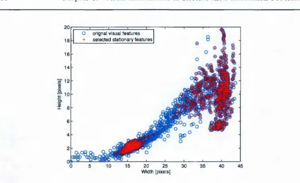
3.3 Visual frame selection scheme ... 58
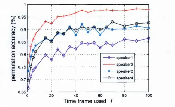
3.4 Permutation accuracy with different number of time f r a m e s ... 62
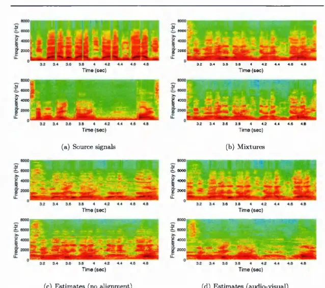
3.5 Spectrograms of the original source signals and their estimates with and without applying the AV sorting sc h e m e ... 63
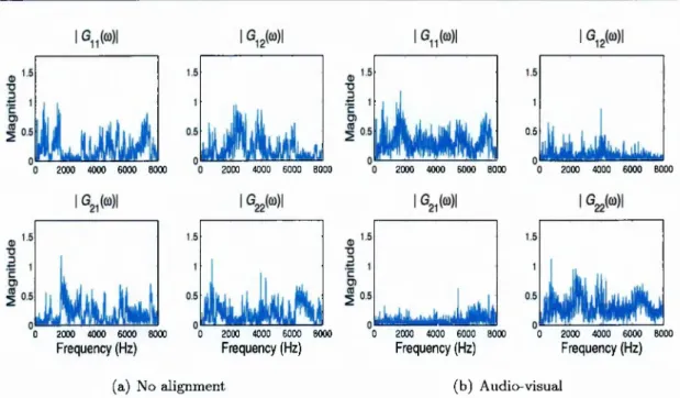
3.6 Global filters in the frequency d o m a i n ... 65
3.7 Plot of |G ii| • IG2 2I — IG1 2I • IG2 1I without n o is e ... 66
3.8 Plot of |G ii| • IG2 2I — IG1 2I • IG2 1I with 10 dB Gaussian white noise . . . 67
3.9 Average SINR m e asu re m e n ts... 69
4.1 Flow of our proposed VAD-incorporated B S S ... 72
4.2 Spectrograms of the original source signals and their estimates after audio-domain B S S ... 76 4.3 Block correlation and energy ratio of the spectra of two source estimates 80
4.4 The two-stage boundaries for interference d etectio n ... 81 4.5 Comparison of our proposed visual VAD algorithm with the
ground-truth, Aubrey et al.’ method and the SVM m e th o d ... . 84 4.6 Spectrograms of the source estimates after VAD-BSS... 87 4.7 SDR evaluations without noise and with 10 dB Gaussian n o i s e ... 90 4.8 PESQ evaluations without noise and with 10 dB Gaussian noise 91
5.1 Flow of our proposed AVDL-incorporated B S S ... 95 5.2 Demonstration of the generative model for A V D L... 98
5.3 Combine and to obtain 109
5.4 The generative atoms and the synthetic d a t a ... 112 5.5 The converged AV atoms learned from the synthetic data using AVDL
and Monaci’s competing m e t h o d ... 114 5.6 The converged AV atoms learned from the synthetic data with extra
convolutive n o i s e ... 115 5.7 The approximation error comparison of AVDL and Monaci’s method
over the synthetic d a t a ... 116 5.8 The converged AV atoms learned from the multimodal LiLIR database
(short sequences) using AVDL and Monaci’s competing m e th o d ... 118 5.9 The converged AV atoms after applying our proposed AVDL algorithm
to the multimodal LiLIR database (long sequences)... . . . 119 5.10 Comparison of the audio mask, the visual mask, the AV mask with the
ground-truth I B M ... 122 5.12 Comparison of the AV mask generated by a symmetrical linear combi
nation with masks in Figure 5 . 1 0 ( b ) ... . 124 5.11 SDR evaluations without noise and with 10 dB Gaussian noise . . . 127 5.13 OPS-PEASS evaluations without noise and with 10 dB Gaussian noise . 128
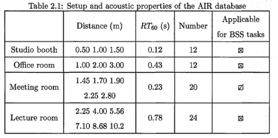
2.1 Setup of the AIR d atab ase... 44
2.2 Setup of the BRIR d a ta b a se ... 45
3.1 Effect of I on SINR ... 68
3.2 Effect of EFT size on S I N R ... 69
5.1 Computational complexity quantisation for AVDL and Monaci’s com peting m e t h o d ... 106
List o f Figures vi
List o f Tables viii
1 Introduction 1 1.1 W hat is B S S ? ... 2 1.2 Why AV-BSS? ... 4 1.3 C o n trib u tio ns... 6 2 Literature Survey 9 2.1 Technical background ... 9 2.2 Audio-domain B S S ... 13
2.2.1 Mixing model categorisation... 14
2.2.2 Instantaneous BSS solutions... 17
2.2.3 Convolutive BSS solutions... 21
2.3 Audio-visual coherence... 27
2.3.1 Visual information categorisation... 28
2.3.2 AV coherence m o d ellin g ... 30
2.4 Audio-visual B S S ... 34
2.4.1 Direct estimation of separation filters ... 36
2.4.2 Addressing audio-domain BSS h m ita tio n s ... 37
2.4.3 Providing additional in fo rm atio n ... 38
2.5 Audio quahty assessment m e tric s ... 39
2.6 Potential applications ... 42
2.7 Database d escrip tio n ... . 43
2.7.1 Mixing filters d a ta b a se ... 43
2.7.2 Multimodal d atab ase... 45
2.8 S u m m a r y ... 48
3 V isual Inform ation to R esolve th e P erm utation Problem 51 3.1 Introduction... 52
3.2 Feature extraction and fusion ... 54
3.2.1 Extraction of audio and visual features... 54
3.2.2 Robust feature frame s e le c tio n ... 56
3.2.3 Feature-level fusion... 57
3.3 Resolution of the permutation problem ... 60
3.4 Experimental r e s u lts ... 62
3.4.1 Data, parameter setup and performance metrics ... 62
3.4.2 Experimental e v a lu a tio n s • • • 64 3.5 S u m m a r y ... 70
4 V isual Voice A ctiv ity D etectio n for AV-BSS 71 4.1 Introduction... 72
4.2 Visual V A D ... 73
4.3 VAD-incorporated B S S ... 76
4.3.1 BSS using IPD and I L D ... 76
4.3.2 Interference re m o v a l... 77
4.4 Experimental r e s u lt s ... 82
4.4.1 Visual VAD e v a lu a tio n s... . . 82
4.4.2 VAD-incorporated BSS evaluations... 85
5 A udio-V isual D ictionary Learning for AV -BSS 93
5.1 Introduction... 94
5.2 Audio-visual dictionary learning (AVDL) ... 96
5.2.1 Coding s t a g e ... 99
5.2.2 Learning s t a g e ...104
5.2.3 C o m p le x ity ... 106
5.3 AVDL-incorporated B S S ... 106
5.3.1 Audio TF mask generation using binaural c u e s ...107
5.3.2 Visual TF mask generation using A V D L ...107
5.3.3 Audio-visual TF mask fusion for B S S ... 108
5.4 Experimental e v a lu a tio n s ...110
5.4.1 AVDL e v a lu a tio n s ...I l l 5.4.2 AVDL-incorporated BSS ev alu atio n s... 120
5.5 S u m m a r y ... 129
6 C onclusions and Future R esearch 131 6.1 C onclusions... 131
6.1.1 Resolve the permutation p ro b lem ... 131
6.1.2 Visual voice activity detection for B S S ...132
6.1.3 Audio-visual dictionary learning for B S S ...133
6.2 Future re s e a rc h ... 134
A List o f A cronym s and Sym bols 137
B List o f Pu blications 143
Chapter
1
Introduction
Real-world phenomena involve complex interactions between elements of a diverse na ture, which can be observed from different sensory modalities, such as vision, hear ing, touch, taste and smell. To enrich perception of the surrounding world, human brains have the ability of multisensory integration, where audio and vision are often involved when it comes to speech interpretation. For instance, looking at the speaker’s lip movements benefits understanding of the utterance, especially in adverse hstening environments. In 1954, Sumby and Pollack [100] wrote:
...if visual factors supplementary to oral speech are utilised, we can tolerate higher noise interference levels than if visual factors are not utilised...the results suggest th at oral speech intelligibility may be appreciably improved in many practical situations by arrangement for supplementary visual ob servation of the speaker.
(Sumby and Pollack 1954)
Sumby and Pollack described the unrecognised visual effect upon speech perception, which was, twenty years later, demonstrated by the famous “McGurk effect” [65], which illustrates th at human brains interconnect the coherent audio and visual modahties rather than deal with them in isolation. A growing body of research has been conducted in the field of audio-visual processing, to facilitate applications ranging from speech
recognition [79, 63, 81], identification [93], enhancement [34], localisation [74], to more recent source separation tasks [97, 109]. Real-world acoustic environments are, most of the time, constituted by the sounds we are interested in as weU as the interfering sources, therefore, the ability to distinguish and separate the source of interest while ignoring irrelevant sounds from their mixtures is of critical importance to guarantee a quick response to changes of the surrounding world. Blind source separation (BSS) [19], which recovers the underlying unknown sources from their mixtures observed at the sensors, is a versatile tool for achieving this separation task. However, existing BSS algorithms are often used in controlled environments in the audio-domain, whose performance deteriorates in adverse conditions with the presence of strong background noise and reverberation. Exploiting the relationship between coherent audio and visual streams and the fact th a t visual information is not affected by acoustic noise, our research is thereby conducted to address the research question, “can the visual modahty be useful for improving the performance of audio-domain BSS algorithm and how?”
1.1
W h at is B SS?
In a room with a number of people talking simultaneously, a human listener with normal hearing abihty can separate and extract the sound of interest from the received sounds picked up by the ears, which are mixtures of multiple competing sounds and other acoustic noise. This phenomenon is termed as the “cocktail party problem” , first introduced by Cherry [23] in 1953. To mimic such separation ability with a robotic system, i.e. the “machine cocktail party problem” , is however extremely challenging, and one solution is proposed under the framework of BSS. So, what is BSS? Cardoso defined it as follows [19]:
Blind signal {source) separation (BSS) consists of recovering unobserved signals or “sources” from several observed mixtures. Typically the obser vations are obtained at the output of a set of sensors, where each sensor receives a different combination of the source signals.
The term “blind” is used since neither the source signals nor the mixing process is known in advance. Not confined to the acoustic domain for separation of speech mixtures, BSS techniques can also be applied in other domains where a sensor array picks up source signals, e.g. radar or sonar signals. However, in this thesis, we consider BSS only for the cocktail party problem.
Hérault and Jutten [45] derived the first unsupervised BSS learning rule, using a re cursive fully interconnected neural network in 1983. Later they defined the adaptive learning rule with the terminology “independent component analysis” (ICA), which ex ploits the mutual independence of the source signals. Since their pioneering work, many ICA-based BSS algorithms [20, 27, 13, 48, 38] have been developed. These algorithms directly obtain the linear demixing filters for separating the independent sources, which work effectively in controlled environments.
Another emerging group of BSS algorithms operate in the time-frequency (TF)-domain using masking techniques [44, 11, 9, 84, 113, 41, 61], i.e., TF points of the same source are grouped together for recovery, where the TF mask indicates the hkelihood of each point originating from a source. The TF masking technique originates from computa tional auditory scene analysis (CASA) [17, 107], which (1) first segregates the sound track into small elements using certain TF representations, and (2) then clusters each element to different sources using cues such as onset, periodicity, harmonicity and com mon locations.
Despite being studied extensively for decades, the performance of existing BSS algo rithms is still limited in real-world acoustic environments. In near ideal conditions, e.g., an auditory scene with a relatively low level of noise and reverberation, the previously introduced algorithms achieve good results th at meet human perception-level require ments. However in adverse conditions, e.g. an acoustic environment where the speakers outnumber the sensors (under-determined), where there exist strong background noise and high reverberation (noisy and reverberant), where the speakers are moving around (time-varying), these audio-domain algorithms deteriorate steadily. Therefore, BSS re mains a scientific challenge th at needs further study, whose modelhng and algorithmic solutions are likely to enlighten a wide range of applications, including hearing aids or
prostheses, human-machine interface, surveillance, and automatic speech recognition.
1.2
W h y AV -BSS?
As stated previously, the performance of the existing audio-domain BSS algorithms is hmited in adverse environments. To improve speech intelligibility corrupted in such conditions, complementary information robust to acoustic noise would be helpful. The intrinsic audio-visual bimodality, weU acknowledged as a basic speech characteristic, might provide such information to assist audio-domain BSS. Indeed, both the audio (auditory) and the video (visual) signals produced by a speaker are the result of the same articulatory gestures, and not surprisingly, the video signal contains additional information to the associated soundtrack, which otherwise might be unobserved in adverse acoustic conditions. For example, use of vision in the form of hp-reading benefits comprehension of a noise-corrupted conversation. Therefore, the visual stream contains complementary information to the audio stream. For instance, Robert-Ribes et al. [87] pointed out th at the phonetic contrasts least robust in auditory perception in acoustic noise were the most visible ones. In addition, a growing body of studies have shown the “audio+speaker’s face” condition improves speech intelligibility compared to the “audio only” situation [100], since human brains integrate the multisensory signals [65, 90, 18, 67] instead of dealing with them in isolation.
The complementary relationship between the coherent audio and visual stimuli forms the basis of audio-visual (AV) speech processing, which has recently been adopted for speech separation tasks, leading to a family of the so-called AV-BSS algorithms. This thesis aims to address the main research question of AV-BSS as stated at the beginning of this chapter, and several sub-questions th at arise as a result, leading to a group of technical challenges:
(1) W hat kind visual information should be used, i.e., how can a reliable audio-visual coherence be modelled?
(2) How to overcome the cross-modal differences between the audio and visual stimuli in size, sampling rates, and dimensionality?
(3) How to fuse the audio-visual coherence with audio-domain BSS algorithms for the separation of reverberant, noisy and under-determined mixtures?
These questions will be studied throughout this thesis, and new AV-BSS algorithms will be proposed. In particular, to assist audio-domain BSS, Question 1 will be addressed via a statistical modelling method using Gaussian mixture models (GMMs) and a sparse representation approach using audio-visual dictionary learning (AVDL), in Chapters 3 and 5 respectively. Visual voice activity information is also used in Chapter 4. Question 2 will be solved by the feature extraction and synchronisation in Chapters 3 and 4, and a sparse structure representation in Chapter 5. Question 3 will be answered using three different paradigms in Chapters 3-5.
The thesis is organised as follows: The background knowledge and a literature review of the related work are introduced in Chapter 2. A novel ICA-based AV-BSS method is presented in Chapter 3, where the AV coherence maximisation is apphed to address the permutation ambiguity, which is related to ICA techniques used in the frequency do main. The proposed algorithm is tested in noisy and relatively low-reverberant environ ments, using data from the multimodal XM2VTS database [1] and another multimodal database containing different combinations of vowels and consonants. In C hapter 4, an AV-BSS algorithm combining TF masking with voice activity cues is developed, which consists of the visual voice activity detection (VAD) training, and the fusion of audio-domain BSS with the detected voice activity cues. Experimental results in noisy and highly-reverberant room environments demonstrate the performance improvement of our proposition, using the multimodal LILiR corpus [94]. Chapter 5 describes an alternative method for modelhng the AV coherence. Rather than globally modelling the joint distribution of the synchronised AV features, a method modelling the lo cal structures of the AV data is proposed, i.e. AVDL, which exploits the temporal structures and sparsity of speech signals. The proposed AVDL is then combined with an audio-domain BSS algorithm for further enhancement, which is also tested on the LILiR corpus in noise and reverberant environments. Chapter 6 concludes the thesis with recommendations for future work. Lists of acronyms and mathematical symbols are also appended, to improve readabihty of the thesis.
1.3
C ontributions
The major contributions of this thesis are summarised as follows:
(1) An AV-BSS method based on ICA and AV coherence maximisation is proposed, which uses the visual information to mitigate the permutation ambiguity, an essential limitation of ICA techniques when applied in the TF domain. In the off-line training process, we characterise statistically the AV coherence using CMMs, whose parameters are estimated via an adapted expectation maximisation ( AEM) algorithm. To eliminate outliers th a t affect the AV coherence modelhng, a robust feature selection scheme is thereby adopted. In the on-line separation process, a novel iterative sorting scheme is developed to address the permutation ambiguity, based on coherence maximisation and majority voting.
(2) A novel audio-domain BSS enhancement method is proposed, which integrates the voice activity information obtained from the video stream. Mimicking aspects of hu man hearing, binaural speech mixtures are considered. In the off-line training process, a speaker-independent voice activity detector is formed via Adaboost training of the manually labelled visual feature vectors. In the on-hne separation process, the TF masking technique is used, which analyses statistically the interaural phase difference (IPD) and interaural level difference (ILD) cues to cluster probabilistically each TF point of the audio mixtures to the source signals. The voice activity cues are also detected via the visual VAD algorithm, and integrated into the TF masking BSS algo rithm via a novel interference removal scheme. Based on Mel-scale frequency analysis, the interference removal scheme is operated in two stages. In the first stage, the inter ference is detected in each block with a strict boundary. In the second stage, in the neighbourhood of the blocks being detected as interference in the previous stage, the residual is detected with a relatively loose boundary.
(3) A new AV-BSS algorithm is developed, which incorporates AVDL into source sep aration and is apphed for the separation of reverberant and noisy mixtures.
In the off-line training process, a novel AVDL technique is proposed for modelling the AV coherence under the sparse coding framework. This new method attempts
to code the local bimodal-informative temporal-spatial structures of an AV sequence. Our proposed AVDL algorithm follows a commonly employed two-stage coding-learning process, and each AV atom in our dictionary contains an audio atom and a visual atom spanning the same temporal length. The audio atom is the magnitude spectrum of an audio snippet while the visual atom is composed of several consecutive frames of image patches, focusing on the movement of the whole mouth region.
In the on-line separation process, the proposed AVDL is integrated into the T F masking technique for enhancement, where two parallel mask generation processes are combined to derive a noise-robust AV mask. The audio mask is generated via T F masking, while the visual mask is generated via AVDL, which are then combined to generate a robust AV mask for extracting the target source from the mixtures, by using a non-linear weighting function.
Literature Survey
2.1
Technical background
Prom the well-known cocktail party problem (effect) [23], we know th at a human with normal hearing ability can extract and focus on one sound of interest from its sound mixtures, while ignoring the other competing sounds and background noise at a multi speaker scenario. To mimic such ability with machines is the so-called machine cocktail party problem, and two popular methods, i.e. computational auditory scene analysis (CASA) and blind source separation (BSS), have been widely used for this purpose. Of which, CASA [17, 107] exploits the mechanisms of the human auditory system by computational means, which is however beyond the scope of this thesis. BSS [45], which is an array signal processing technique th at recovers the unknown sound sources from their observed mixtures, is exploited due to its versatility and computational efficiency. The term “blind” refers to the fact th at there is very limited or no prior information available, about the sources or the mixing process. In other words, BSS is an un-supervised machine learning problem, which optimises the output using only the information observed at the mixtures and no off-line labelled training is needed. BSS has a wide range of apphcations for the processing of e.g. radar signals, medical images and financial time series. In this thesis, we only focus on the use of BSS for speech source separation tasks.
better understanding of the techniques behind different BSS methods, the basic m ath ematical and statistical concepts are briefly introduced as follows. The first one is related to statistics, which are measures of some certain attributes of a stationary sig nal X with the distribution f( x) . Stationary means th at f ( x ) does not change with the increasing number of samples. More specifically for a time series such as a noise or sound signal, the stationarity or non-stationarity exhibits time-invariant or -varying statistics. Different statistics can be calculated using different functions, for example, the mean p = x f ( x ) dx, the variance cr^ = (x — p)^f (x) dx, and the i-th standardized moment f ( x ) dx. Specifically if i > 2, the z-th moment is ref-ered to as a high-order statistic. When z = 3, it is the skewness th at measures the symmetry of f{x)', when i = 4, whose value minus three is the kurtosis th at measures the shape of f{x). Very similar to moments, cumulants are another sets of statistics and provide an alternative way to evaluate a distribution. Both the high-order mo ments and high-order cumulants are often exploited in BSS systems. To reduce the computational complexity, pre-whitening, or “standardisation” as named in [27], is of ten applied before applying BSS, which removes a set of low-order terms in high-order statistics. Pre-whitening decorrelates a multivariate signal x = [xi,X2, ..., xp]'^, and transforms it to a space with a unit covariance: E'{zz^} = I, where the superscript T denotes transpose and z = B x is the decorrelated signal with the transformation matrix B. This pre-whitening process can be viewed as principal component analysis (PCA) based on singular value decomposition (SVD) of x or eigenvalue decomposition (EVD) o fx x T
Gaussian white noise (OWN) has very special statistics with a normal (Gaussian) dis tribution f {x) = exp —( ^ ^ ) ^ . Moments of high orders (higher than two) are specified values for GWN while its cumulants beyond the first two are zeros. As op posed to the Gaussian distribution whose kurtosis (the forth cumulant) is zero, the Super-Gaussian distribution has positive kurtosis, and visually it has heavy tails, such as the Laplacian distribution. Speech signals are super-Gaussian. A sub-Gaussian dis tribution such as the uniform distribution, in contrast to super-Gaussian, has negative kurtosis and visually thin tails. The term “white” in GWN means th at all frequency components are present in the spectrum with equal energy, as in white fight. Coloured
noise, as opposed to the “white” noise, yields variation in the spectrum. Another term associated with “white” is “non-whiteness” , which denotes the spectrum of a stationary process have different values at different frequency bins, i.e., different auto-correlation coefiicients at different time-lags.
As mentioned previously, statistical cues of source signals are often exploited by BSS techniques. However, for speech signals, direct estimation of the above statistics may result in errors, since they are non-stationary, i.e. their distribution and statistics vary with time. One solution is to convert them to some transform domain. Fortunately, speech signals are quasi-stationary, or short-term stationary, which means a signal is overall non-stationary and can be approximated as stationary in a short time period. Therefore, speech signals can be converted into the time-frequency (TF) domain based on quasi-stationarity, which is a representative domain of time sequences after applying short-time Fourier transform (STFT). STFT can be achieved by first segmenting a time series into parallel blocks and then applying Fourier transform to each block. In the T F domain, statistical cues such as independence cues can be exploited.
Bell and Sejnowski [13] categorised BSS into two types [13]. In the first type of BSS algorithm, neural networks with Hebbian-type learning are exploited. Neural networks are information processing paradigms inspired by animal central nervous systems, i.e. brains, which are widely used in the field of machine learning and pattern recognition, where a set of neurons (non-hnear functions) work in unison to solve specific problems. Hebbian-type learning is an un-supervised learning algorithm based on only local infor mation, which is self-organised to detect the emergent collective properties. Therefore, such a neural network learns and operates simultaneously, which is adapted to on-line data rather than dealing with data in batch mode. In the second type of BSS algorithm, specific contrast functions are optimised. A contrast function is continuous-valued, non quadratic and depends only on a single extracted output signal; whose maxima under suitable source or coefficient constraints correspond to separated sources [59]. An ex plicit contrast is generally characterised by high order statistics, such as moments and cumulants measured from data in batch mode.
component analysis (ICA) and TF masking respectively. In the first BSS algorithm, the ICA [27] technique is used, which is a computational method for separating a multivariate signal into additive subcomponents. There are two assumptions applied to the multivariate signal as follows. (1) Each variable Xi in the multivariate signal is assumed to be non-Gaussian. (2) Different variables X{ and xj are mutually or pairwise independent from each other, which means the joint probability p(xi,Xj) is the products of their marginal probability p ( x i )p (x j) . Entropy, a measure of disorder, can be used to evaluate the Shannon mutual independence from information point of view. In the second BSS algorithm, TF masking is used, which originates from CASA. The TF masking technique keeps or attenuates the audio information of the mixture by applying a factor at each TF point, and all the factors associated with the recovery of one source signal form a TF mask. If each factor value is either 0 or 1, then a binary mask is generated. Otherwise, a soft mask is generated with each factor value spanning between [0 1].
However, one limitation of the existing BSS algorithms is th at their performance de grades steadily in adverse environments, e.g. with the presence of a high level of noise and strong reverberation as well as multiple competing speakers. To improve the in telligibility of noise corrupted speech, additional information th at is complementary to the audio input is highly desirable. Vision, not affected by acoustic noise, contains such promising information due to the bimodal nature of speech signals, for both the speech production and perception processes [65]. This promising additional visual information about the audio modality, i.e. the complementary relationship between concurrent au dio and visual streams originating from the same event, is termed as the audio-visual (AV) coherence. Using the AY coherence to assist traditional BSS is an emerging ap plication in the field of joint AV signal processing, leading to a family of the so-called AV-BSS algorithms.
We need to stress that, although there are advantages of using visual cues to assist BSS, there are also some limitations. For instance, there is a strict requirement to the quality of the video, distorted video such as blurred or low-resolution videos therefore may degrade the AV-BSS performance. Also, in some cases, the visual cues may mislead the corresponding audio part, which is also demonstrated in the McGurk effect [65]
when the visual /g a / plus an audio /h a / leads to the wrong perception of /d a /. We assume the quality of visual sequences is good enough to benefit rather than degrade the performance of BSS systems.
Another limitation is th at AV-BSS algorithms are often accompanied with an off-line training process, which implies they cannot handle cases where no training set about the target source(s) is available. This training process aims to model the AV coherence, which works as a prior information for BSS systems. As we have stressed previously, BSS algorithms are called “blind” since there is no prior information available. There fore, the additional information coming from the AV coherence, to some extent, makes the BSS methods less blind. Nevertheless, we still use the name AV-BSS instead of AV-SS, since the former has been commonly used. AV coherence modelling can be achieved by different mathematical tools, e.g., statistical characterisation of the joint AV probability in the synchronised AV feature space, visual voice activity detection (VAD) and audio-visual dictionary learning (AVDL) to capture the tem poral struc tures. Of which, the AVDL technique involves both audio and visual modalities, in contrast to the normal dictionary learning algorithms applied to monomodal data. A novel AVDL algorithm is proposed in Chapter 5, and one essential novelty of our propo sition is the utilisation of locality constraints with analytical solution as opposed to the commonly-used sparse-coding strategy. In other words, our proposed AVDL resembles the properties of locality-constrained linear coding (LLC) widely used in image coding, which utilises the locality constraints to project each descriptor into its local-coordinate system, and the projected coordinates are integrated by max poohng to generate the final representation.
2.2
A udio-dom ain B SS
A general introduction of the technical background is first given, to help the readers to understand the basic mathematical and statistical concepts and definitions used in this thesis. Before we continue to introduce the existing BSS algorithms in detail in this section, we need to stress the general setting throughout this thesis. Firstly, the simplest 2 x 2 cases are considered for the ease of understanding, i.e., two microphones
and two speakers, which can be generalised to the condition with multiple microphones and speakers. To mimic human hearing scenarios, the two microphones are allocated at the positions of two ears using a dummy head. Secondly, real-room environments are considered which involve reverberation and background noise. We consider the ideal situation when both the listener and the speakers are immobile, i.e., moving around and head rotations are not allowed, which exhibits a time-invariant mixing process. Thirdly, of the two source signals, one is supposed to be the target and the other as interference, and we are only interested in the target speech. As a result, evaluations of BSS algorithms are apphed to the target signal while ignoring the competing speech.
The performance of existing BSS methods relies strongly on the complexity of the mixing model, i.e., how the sources are mixed within the “cocktail party” scenario, as discussed next.
2 .2 .1 M ix in g m o d e l c a te g o r isa tio n
Typically in a cocktail party environment, there are multiple concurrent active speakers, as well as some background noise such as clinking of glasses and light music. Due to the surface reflections in rooms and the propagation of sound in air, sound sources and interference come to a listener’s ears from both direct and reverberant paths, as demonstrated in Figure 2.1. So the question is how can we model the mixing process for machines to accommodate the diffuse surface reflections, noise and other complex constraints in an enclosed room?
Assuming an ideal noiseless anechoic environment where the sounds directly come to the microphones without being distorted by noise and reverberation, we can consider the simplest mixing model, additive mixing or instantaneous mixing. In such conditions,
K unknown source signals {&&(?%)}, 1 < k < K are scaled and added with different combinations to yield P observations {^p{n)}, 1 < p < P:
K
= ' ^ k p k Sk ( n) , (2.1a)
k=l
Noise Mlc 1
Speaker 2
Figure 2.1: A simplified cocktail party scenario with two speakers and two sensors, where the two sensors (microphones) mimic aspects of a listener’s ears.
where hpk represents the contribution of source k to sensor p. Equation (2.1b) represents the matrix form of the additive mixing process, where x(n) = [xi{n), ...,xp{n)]'^ is the observation vector, s(n) = [si(n), ...,s/^(n)]^ is the source vector at the discrete time indexed by n where H = (hpk) 6 is the unknown non-singular matrix, assumed to be time-invariant.
The additive mixing model has limited practical applicability in real-room BSS tasks, where the reverberant acoustic paths yield a more practical and commonly-used con-volutive mixing. In such conditions, the sources are convolved with different room impulses and collected by the sensors:
K +00
Xpiri) ^ ^ ^ ^ hpiç(^q^Sjç(^n ç), (2.2a)
k = l q = —oo
x(n) = H * s(n). (2.2b)
where H = (hp^) is the mixing tensor with its {p,k)-th element hpk — (hpkiq)) being the mixing filter from source k to observation p and * denotes convolution. For a physically realisable (causal) system, the tap index q of each mixing filter hpk should start from 0 and have an upper bound, depending on the reverberation time. This is often measured by the reverberation time RTqo [89], when reflections of a direct sound decay by 60 dB below the level of the direct sound.
There are also some other issues related to the mixing process. For example, depending on the sensor number P and source number A , BSS mixtures are categorised into over
determined, even-determined and under-determined situations, with P > K, P = K, P < K respectively. The under-determined BSS problem is the most challenging one, since the system is not invertible, and one cannot estimate the demixing filters even given the mixing filters. Considering whether the noise is present in the environment, we have noise-free mixtures and noise-corrupted mixtures. In addition, the noise might be stationary such as Gaussian white noise, or non-stationary and coloured such as speech-hke interference. Also, the speakers and listeners are mobile, i.e., they may rotate their heads and move around during a conversation, which results in a time- varying mixing process as compared to the generally considered time-invariant systems. These situations are much more complex and are beyond the scope of this thesis.
si(n)
►
U n k n o w n
^ ^
S o u rc e
^
m ixing
x.(n)
separation
S2(n)---► ® ^ ^ y z W
Unknown sources Observations Source estim ates
Figure 2.2: Schematic diagram for a typical 2 x 2 BSS system.
Based on different mixing models, different BSS techniques have been developed in the audio domain, exploiting the spatial diversity and characteristics of the sound sources, such as non-stationarity [62, 24, 25, 114], quasi-stationarity [96], non-whiteness [103, 14, 68], non-Gaussianity [20, 39], mutual independence [45, 27, 13, 19, 38], and modelling of other cues such as spatial cues [112, 61, 57, 41]. The schematic diagram of a typical 2 x 2 BSS system is shown in Figure 2.2. Despite of the use of increasingly complex mixing models mentioned above, solutions to instantaneous BSS are the most basic ones, which can be generalised to other complex mixing scenarios via, for example, Fourier transforms. Many instantaneous BSS algorithms have been developed and introduced in detail as follows.
2 .2 .2 I n sta n ta n e o u s B S S s o lu tio n s
Based on the assumption th a t speech signals are uncorrelated stationary ergodic pro cesses, Non-whiteness is an important characteristic of speech signals since they have different magnitudes at different frequency bins, leading to a family of BSS algorithms [103, 14, 68] th at jointly diagonalises the correlation matrices at different time-lags. Tong et al. proposed the algorithm for multiple unknown signal extraction (AMUSE) [103], which involves the successive eigenvalue decompositions of sample correlation matrices, whose solutions get asymptotically close to the least squares source esti mates with an increasing number of measurements. Molgedey et al. [68] successfully separated sources from their (non-)linear mixtures, with simultaneous diagonalisation. Belouchrani et al. proposed second-order blind identification (SOBI) [14], which jointly diagonalises an arbitrary set of correlation matrices, which is a generalisation of the Jacobi technique for the exact diagonalisation of a single Hermitian m atrix [35]. Unlike AMUSE, SOBI allows the separation of Gaussian sources.
Non-stationarity is an essential nature of speech signals, since the statistical properties of their frequency representation change continuously with time. As a result, variances of the source signals are also non-stationary, which is particularly evident when com paring them between silent and active periods. Matsuoka et al. [62] proved th a t such a variance allows the estimation of source signals, and developed a BSS algorithm using neural networks to decorrelate the source estimates. Choi and Cichocki also state th a t [24] “the second-order correlation matrices of the data calculated at several different time-windowed data frames are sufficient for BSS when sources are non-stationary” . As a consequence, a series of decorrelation-based algorithms [24, 25,114] were proposed for instantaneous mixtures, which utilises the joint diagonalisation of several correlation matrices at different time-instants.
The previously introduced BSS algorithms involve explicitly or implicitly the decor relation of a set of covariance matrices. Another set of BSS algorithms decorrelates the sources with high order statistics, which exploits the mutual independence between source signals. These algorithms form the well-known technique called independent component analysis (ICA) [45, 27, 19, 38]. The decorrelation-based BSS algorithms
are equivalent to using ICA techniques up to the second order, in other words, ICA is a higher-order generalisation of principal component analysis (PCA) [27, 39]. For Caussian-distributed source signals, ICA is equivalent to an orthogonal transformation, since high order statistics of Caussian distributed signals are fixed values [39].
ICA aims to find a separation filter, W , for an instantaneous mixture in Equation (2.1) to make the output y(n) as mutually independent as possible,
y(n) = W x(n). (2.3)
Several assumptions are often made to address the ICA problem as follows.
(1) Even-determined or over-determined mixtures where the number of the observa tions is equal to or greater than the number of the underlying sources. More strictly speaking, columns of the mixing filter H in Equation (2.1b) are assumed to be linearly independent. In such cases, the separation filters can be calculated directly from the estimated mixing filters for source separation [19]. Pre-whitening, is often applied to decorrelate the mixtures, and one of its by-products is th at the over-determined cases are transformed to even-determined mixtures. However for the under-determined situ ations, which are not invertible, there does not exist a linear solution for the separation filters even if the mixing filters are known.
(2) Non-Caussianity or up to one Caussian assumption of the sources. Often the third- and the fourth-order statistics (i.e. moments and cumulants) are exploited in ICA. However for Caussian-distributed signals, moments of high orders (higher than two) are specified values while cumulants beyond the first two are zero, which do not contribute any information. As a result, they cannot distinguish two or more Caussian sources. Bell and Sejnowski [13] explained this problem in a more straightforward way th a t “the sum of two Caussian variables has itself a Caussian distribution”.
(3) Last but most importantly, mutual independence between the source signals. The essential objective of ICA is to make the source estimates as mutually independent as possible. Therefore, the independent outputs after ICA are not genuine copies of the original sources, if the sources are dependent with each other. Fortunately different speech signals can be considered as mutually independent [59].
Bell categorised the ICA technique into two different types. One is through neural net works with unsupervised online Hebbian-type learning, as represented by the pioneering work of Jutten and Hérault [45] in 1983. The other one is through unsupervised learn ing in batch mode, which uses explicit estimation of cumulants as the independence criteria, as represented by Comon’s ICA method [27].
The first type of BSS algorithm is from a neural processing perspective. The adaptive H-J algorithm [45] successfully cancels the non-linear cross-correlations of instanta neous mixtures in a simple feedback architecture. Since independence involves the uncorrelatedness of the outputs th at have been applied with non-linear functions, the H-J algorithm th at cancels the non-linear cross-correlations produces independent com ponents, with carefully chosen non-linearities depending on the assumed source distri butions. Even though it lacked a convergence proof when it was proposed, it is the first adaptive learning rule to address the ICA problem. The reason for its success lies in the information-theoretic learning rules th at maximise the mutual information between the mixtures and the outputs, i.e. the information maximisation (Informax) principle as proposed by Linsker [51], further refined by Amari et al. with a natural gradient optimisation [6, 5]. Bell and Sejnowski [13] proved th at the Informax principle was equivalent to the maximisation of the output entropy for an invertible linear mix ing process, and thus derived an unsupervised online learning rule through non-linear sigmoidal neurons, without any assumption of the input distribution. Their proposed algorithm provides relatively robust performance and efficiency for super-Gaussian dis tributed sources. The Informax was later extended to mixed sub- and super-Gaussian distributed signals by Lee et al. [48].
Another widely used neural ICA algorithm is the fixed-point FastICA algorithm [38, 37] proposed by Hyvarinen and Oja. Strictly speaking, it is not an on neural algorithm, since it deals with data in batch mode. However, due to its parallel and distributed structure, as weU as its efficient computation th at requires little memory space, it can still be considered as a neural algorithm. By choosing different non-linearities, a set of kurtosis-based FastICA algorithms is developed. FastICA shows appealing quadratic convergence properties, or even cubic convergence when the source densities are symmetric.
For the second type of BSS algorithm, the independence is explicitly evaluated by a statistical metric such as a contrast function. From an information-theoretic view point, different contrast functions have been used based on different criteria, including the maximum likelihood (ML) principle [19], mutual information minimisation [27] or negentropy maximisation [38]. The ML principle can be used to estimate the parame ters of an underlying statistical model, based on hypothesis about the distribution of the sources. Note, unlike the mutual information as defined in the Informax principle [51] as introduced previously, the mutual information here is evaluated only on the outputs, and its minimisation is equivalent to minimising the sum of the entropies for each output component. These above contrast functions are evaluated on high order statistics, often in the form of cumulants of increasing orders. Focusing on the alge braic properties of the fourth-order cumulants exploiting non-Gaussianity of the source signals, Cardoso et al. proposed a computationally efficient joint approximate diago- nahsation of eigenmatrices (JADE) algorithm [20], where the joint diagonalisation of a set of fourth order cumulant matrices yields the ICA estimates, whose optimisation is achieved by Jacobi rotations. Comon [27] approximated the mutual information evalu ated by the Kullback-Leibler (KL) divergence with Edgeworth expansion of third- and fourth-order marginal cumulants, and his algorithm shows convergence and robustness, even in the presence of strong non-Gaussian noise. Afterwards, the optimisation of the contrast functions, can be achieved by gradient descent algorithms or more sophisti cated Newton-like algorithms.
Note that, there is one intrinsic limitation of the ICA techniques [13, 38, 20, 27]: th at they suffer from indeterminacies of both scale and order, i.e., the estimated independent components are copies of the original independent sources up to different scales and permutations. Comon [27] proved this phenomenon for any contrast of polynomial form in marginal cumulants. This is the well-known scaling ambiguity and permutation ambiguity of ICA:
y(n) = D P s(n ), (2.4)
where D is a diagonal matrix denoting that the source estimates are scaled versions of the original sources, and P is a permutation matrix denoting that the order of the source estimates may not be consistent with the original one.
The previously introduced BSS methods for instantaneous models are limited in real- world environments, where more complex convolutive models are considered due to multi-path sound propagation and room reverberation, as introduced next.
2 .2 .3 C o n v o lu tiv e B S S so lu tio n s
Convolutive mixing models in Equation (2.2) are often considered for real-room mix tures, where the observations are corrupted by room reverberation. To solve this prob lem, time-domain deconvolution algorithms [111, 47, 7, 102, 66] can be apphed. How ever, the time-domain methods are computationally expensive, especially when the mixing filters have long taps. Moreover the inverse of the mixing filters, i.e. the sepa ration filters, may become ill-conditioned in the case of multipath (reverberant) effects, which may result in the loss of identifiabihty. One solution to this challenge is to trans form the time-domain signals to some other domains, in such a way th at the convolutive model becomes a set of parallel instantaneous models, so that the existing separation tools for instantaneous BSS [103, 14, 13, 48, 38, 20, 27] can be used. Fortunately, speech signals are short-time stationary (quasi-stationary), which is the basis of block processing, via, e.g. the most commonly-used short time Fourier transform (STFT) [96, 109, 85, 55, 56, 8, 40, 73, 62, 80, 92]. For instance, STFT can be applied to the m -th short-term signal 5(771, 72) segmented from the original signal 5(72), to obtain the
spectrum in frequency bin w and time frame m:
5 (772, w) = ^ ”(5(772,72)).
Another advantage of the STFT representation is th at the mixtures become more sep arated than those in the time-domain. Consequently, each time-frequency (TF) point can be clustered to a single source (assuming th at only one source is dominant at each TF point of the mixture) with TF masking techniques.
In the following two subsections, we will focus on two frequency-domain BSS (FD-BSS) methods. The first method is based on parallel ICAs in different frequency bins, while the second one uses TF masking techniques exploiting sparsity of the spatial cues. Both methods have been used in our work. We need to stress that, we consider only
2 x 2 cases in this thesis for the simplicity of understanding, and evaluations of the BSS algorithms are focused on the target speaker. However, both sub-classes, as will be introduced subsequently, can be generalised to more than one competing speakers. The T F masking-based BSS algorithm is constrained to a particular setting of sensors positioned around a dummy head. The thesis only considers even-determined BSS problems which cover over-determined BSS problems, even though the TF masking- based method is available for the underdetermined situations.
F D -B S S b a se d on IC A
After applying STFT to each of the observed signals, we get an instantaneous mixing model in each frequency bin w ignoring the noise and convolutive components extending beyond the duration of the analysis frame,
X(m,uj) = Jî{u})S{m,üj), (2.5)
where X { m , u ) = [Xi(m, a;),..., A'p(m,o;)]^ is the observation vector in frequency bin
uj and time frame m, and H(w) is the Fourier transform of the time-invariant mixing filters. Then in each frequency bin w, an ICA [27] for instantaneous models is applied to obtain the independent outputs Y (m, u) = [yi(?n, w ),..., y)^(m, w)]^, i.e. the estimates of the source components at each frequency bin:
Y ( m , u ) ='W{cjj)X{m,oj) = S {m ,u ). (2.6) Since the mixing filter H(w) is time-invariant, its inverse separation filter W(w) should also be time-invariant, i.e. not dependent on time index m. Separated components at each channel associated with the same source are then grouped together and trans formed back to the time-domain via inverse short time Fourier transform (ISTFT), for generating the source estimates.
However, at different frequency bins, the ICA-separated components are inconsistent in their order and scale, caused by the indeterminacies as introduced in Equation (2.4) in the previous subsection.
The inconsistency of the scale at different frequency bins results in the scaling problem. Take a 2 x 2 convolutive system for example, the ICA-separated components may have
inconsistent scales such th at at different frequency bins when u j = 1,2, . . . , ! ) :
, . . . , for all m,
Si (m ,l) aiiSi (m,2)
¥2(171,1) _ _S2(m,l) ) }^(Tn,2) «2 2% (771,2)
where a n and 0 2 2 represent linear filters with unknown weights, probably not equal
to 1. Consequently, if we directly apply the ISTFT to the first components for all the frequency channels and collect them into one source, i.e., [si(:, 1), a n s i( :, 2),...], the recovered source would be distorted (coloured) by some non-hnear filter. This is the so called scaling ambiguity associated with FD-BSS, which introduces self-distortion.
In the same way, if the ICA-separated components have inconsistent orders
, . . . , for all m. 'Y i { m ,i y Si (m,l) ¥ i(m ,2) S2 (m,2)
¥2(771,1) S2(m,l) 5 Y2(m,2) Si (m,2 )
The first components in each channel, [5i(:, 1), S2(b 2),...], would contain spectral in
formation from both sources. This is the well-known permutation problem th at results in cross-distortion.
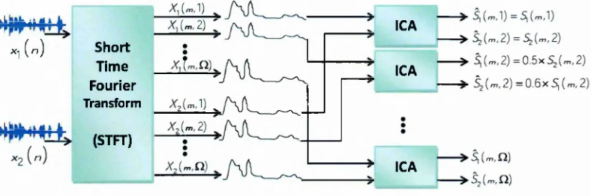
The diagram of a typical ICA-based FD-BSS method is shown in Figure 2.3, the asso ciated scahng and permutation problems are also illustrated.
XI (n) S h o rt Tim e Fourier Transform (STFT) ICA ICA ICA
Figure 2.3: Schematic diagram for a typical 2 x 2 FD-BSS system based on parallel ICAs. Independent ICAs are applied at different frequency channels before the sources are reconstructed in the time domain. The permutation and the scaling ambiguities are demonstrated in the outputs of the first two channels, i.e. when w = 1 and w = 2, and Q is the total number of the frequency channels.
Compared to the self-distortion caused by the scaling ambiguity, which is equivalent to filtered versions of the original sources, the permutation problem results in more severe
(indeed intolerable) distortion in the form of crosstalk interference between sources, which is also a technical challenge we want to address in Chapter 3. These ambiguities need to be addressed before the reconstruction of the sources in the time domain. To mitigate the scaling problem, the minimal distortion principle (MDP) [62, 92] can be applied.
To address the permutation problem, many algorithms [8, 80, 40, 73, 92, 64, 82] have been proposed. For example, the approach in [8, 80, 82] utilises the continuity of the spectral components in adjacent frequency channels, which assumes there is some interconnection between different frequency bins. The method in [40, 73] uses direction of arrival (DOA) estimation, where DOA denotes the direction of a propagating wave reaching to a sensor array, which is caused by the propagation models of sounds in air and can be modelled by beamforming techniques. The algorithm in [92] combines both of the above cues, and [64] utilises statistical signal models. Of the de-permutation algorithms mentioned above, the methods proposed by Pham et al. [80] and Pahbar et al. [82] respectively are very popular ones.
Principles of Pham ’s proposition are as follows. Suppose the time-centred profile for the k-th source estimate as at the (m, w)-th time frame is denoted as
E'k(m,uj) = \\Y k{ m ,u )f - Ek(uj),
where F'^(w) is the mean of ||y^(m, w)j|^ over time. Denote as the mean of
Ei^(m,u) over frequency, then the permutation matrix in the w-th frequency bin can be estimated by minimising the following objective function:
D{u) = argmmY^\\Ek{rn,uj) - E k { m ) f .
° k,m
This profile calculation and the permutation estimation processes are iteratively done in a bootstrap way until convergence.
In Pahbar’s method, cross-frequency correlation between neighbouring frequency bands is calculated based on a multi-level hierarchical structure, with the assumption th at signal profiles in different bands undergo interrelated changes. In each level, all the frequency bins are grouped to different subsets, and each subset contains two sets of
neighbouring frequency bins. The bottom layers have fine resolutions while the top layers have coarse resolutions. De-permutation is then done by minimising the cross correlation of the associated spectra for each subset. A bottom-to-top flow is applied in the de-permutation scheme.
The above methods are straightforward to implement, and work efficiently for con trolled environments with a low level of noise and reverberation. However in adverse conditions, the utilised properties such as inter-spectral continuity are corrupted by strong noise and reverberation. As a result, the de-permutation performance deteri orates rapidly. In our work presented in Chapter 3, the visual stream, which is not affected by acoustic distortions, is exploited to address the permutation problem.
FD -B SS using T F m asking
Another emerging set of FD-BSS algorithms uses the TF masking technique which clusters each TF point of the mixtures to different sources, where the value of each TF point of the mask indicates the probability of this point coming from a source sig nal. T F masks are estimated from the mixtures via the evaluation of different cues such as onset, periodicity, harmonicity and spatial positions [112, 61, 57, 41]. W ith the assumption th at different sources are disjoint to each other in the TF domain, a hard binary mask [44, 11, 9, 84, 113, 41] can be generated if the prior knowledge of which source occupies each TF point is known. This binary mask is ideal, if the prior knowledge is accurate, e.g. when the contributions of each source to the mixtures are provided. However this disjoint assumption of the sources does not hold for reverber ant mixtures, where different sources contribute partially to each TF point with one dominant source. Therefore, an alternative to the hard binary mask is the soft mask [61, 57], where instead of having a binary value of 0 or 1 for each T F point, a value between [0 1] is obtained to show the proportion of this point belonging to a partic ular source, based on the statistical evaluation of the separation cues. For instance, binaural mixtures are considered in our proposed system in Chapters 4 and 5 to mimic aspects of human hearing. Mandebs state-of-the-art audio-domain BSS method [61] is introduced, exploiting the binaural cues [112] of interaural phase difference (IPD) and
interaural level difference (ILD). The principles of Mandel’s method are summarised as follows.
A source signal arrives at two ears with different time delays and attenuations:
L { m , u ) / R { m , u ) = 10 ^20 ^ ç3Krn,u})^ (2.7)
where L(m,uj) and R{m,uj) are the TF representations of the left-ear and right-ear signals respectively, at the T F point indexed by Two Gaussian distributions are used to model the ILD o;(m,a;) and IPD p{m,oj) for source k at the discretised time delay indexed by r:
P iP D ( m ,a ;|f c ,r ) ~ A /'(4 ^ ( o ; ) ;o - |^ ( a ;) ) ,
(2.0)
P i L D { m , u \ k )
where PiPD(?rt, u\k, r) and pn.D{m, uj\k) are respectively the likelihood of the IPD and the ILD cues at the TF point (m, w) originating from source k at time delay r , parametrised by the means and variances 0 = % T (^), o"^^(w), //;^(w), ?;^(w)}. W ith the independence assumption of ILD and IPD, the likelihood of the point (m, w) originating from source
k at delay r is
P i p d / i l d ( ^ , (^\k, t ) = PiPD(m, uj\k, T )p iL D (? 7 % , u\k)i.pkT, (2.9)
where (pkT is the overall posterior probability of a TF point coming from source k at delay r , as calculated in Equation (2.11a). Under the expectation maximisation (EM) framework, the parameter set 0 can be estimated as shown in Algorithm 1.
After convergence, source k can be estimated from either L(m,uj) or R ( m ,u ), by e.g.
Sk{m,u}) = X^^p(fc,r|m,o;)L(m,a;). To recover sources from only one ear signal how ever may cause information loss. Consequently, the TF mask is applied to both signals to obtain their average as the source estimate in our work.
The above mentioned audio-domain BSS techniques work well in controlled environ ments, e.g., where the mixtures are instantaneous or with a relatively low level of reverberation, noise-free or with a negligible level of noise, and there are only a small number of competing speakers adequately separated in space. However, the quality of BSS-separated speech signals degrades dramatically in adverse environments. To
A lg o rith m 1: F r a m e w o r k o f t h e E M m e t h o d . In p u t: ILD a{m,uj) and IPD p(m,uj), initialised 0 . O u tp u t: Optimised parameter set 0 .
1 In itia lisa tio n : iter = 1.
2 w hile iter < M a x l t e r do % E s te p
Posterior calculation:
% M s te p
Parameter set 0 update:
iter = iter + 1.
address this problem, additional information th at is complementary to the audio input is highly desirable. As introduced previously, there is a complementary relationship between concurrent audio and visual streams, i.e. the AV coherence. The AV coher ence contains promising information robust to acoustic noise, which might be useful to assist BSS systems in adverse conditions, as introduced next.
2.3