Clemson University
TigerPrints
All Dissertations
Dissertations
5-2013
Robust and Efficient Regression
Qi Zheng
Clemson University, [email protected]
Follow this and additional works at:
https://tigerprints.clemson.edu/all_dissertations
Part of the
Statistics and Probability Commons
This Dissertation is brought to you for free and open access by the Dissertations at TigerPrints. It has been accepted for inclusion in All Dissertations by an authorized administrator of TigerPrints. For more information, please [email protected].
Recommended Citation
Zheng, Qi, "Robust and Efficient Regression" (2013).All Dissertations. 1107.
ROBUST AND EFFICIENT REGRESSION
A Dissertation Presented to the Graduate School of
Clemson University
In Partial Fulfillment of the Requirements for the Degree
Doctor of Philosophy Statistics by Qi Zheng May 2013 Accepted by:
Dr. Colin Gallagher, Committee Chair Dr. Karunarathna B. Kulasekera, co-advisor
Dr. Chanseok Park Dr. Xiaoqian Sun Dr. Robert Taylor
Abstract
This dissertation aims to address two problems in regression analysis. One problem is the model selection and robust parameter estimation in high dimensional linear regressions. The other is concerning developing a robust and efficient estimator in nonparametric regressions.
In Chapter 1, we introduce the robust and efficient regression analysis, discuss those two interesting problems and our motivations, and present several exciting results.
We propose a novel robust penalized method for high dimensional linear regression in Chap-ter 2. Asymptotic properties are established and a data-driven procedure is developed to select adaptive penalties. We show it is the very first estimator to achieve desired oracle properties with certainty for high dimensional linear regression. Extensive simulations have been conducted and demonstrate the usefulness of the new technique.
A new local polynomial nonparametric regression is developed in Chapter 3. It minimizes a convex combination of several weighted loss functions simultaneously. The optimal weights are selected by a proposed procedure and adapt to the tails of the error distribution resulting in a procedure which is both robust and resistant. The asymptotic properties have been investigated. We show the resulting estimators are at least as efficient as those provided by existing procedures, but can be much more efficient for many distributions. Its excellent finite sample performance is presented through simulations under a variety of settings. A real data analysis exhibits the usefulness of the proposed methodology.
Dedication
I dedicate this work to my loving parents. It is their love and support that made this work a complete one.
Acknowledgments
I would like to express my gratitude to many individuals who helped me in many ways during this work.
First and my foremost, I am indebted to my co-advisors Drs. C. Gallagher and K.B.Kulasekera for their guidance and support. Their mathematical insights inspired me and helped me make this a success.
I would also like to thank Drs. C. Park, X. Sun, and R. Taylor for their insightful suggestions. Last but not least, I would like to thank the Department of Mathematical Sciences for providing me financial support during my Ph.D studies.
Table of Contents
Title Page . . . i Abstract . . . ii Dedication . . . iii Acknowledgments . . . iv List of Tables . . . viList of Figures . . . vii
1 Introduction . . . 1
1.1 High dimensional linear regression . . . 2
1.2 Adaptively weighted kernel regression . . . 3
2 Adaptive Penalized Quantile Regression for High Dimensional Data . . . 5
2.1 Introduction . . . 6
2.2 The adaptiveL1 quantile regression . . . 7
2.3 Asymptotic Properties . . . 9
2.4 Numerical analysis . . . 13
2.5 Conclusion . . . 14
3 Adaptively Weighted Kernel Regression . . . 16
3.1 Introduction . . . 16
3.2 The adaptively weighted local polynomial regression . . . 18
3.3 Asymptotic Properties . . . 20
3.4 Numerical Studies and Applications . . . 28
3.5 Conclusion . . . 33
Appendices . . . 34
A Proofs for Chapter 2 . . . 35
B Proofs for Chapter 3 . . . 43
C Supplemental Material . . . 49
List of Tables
2.1 Simulation results for model 1 . . . 13
2.2 Simulation results for model 2 . . . 14
3.1 Simulation results for model 1 . . . 29
List of Figures
3.1 Scatter plot and three fittings . . . 31 3.2 Outliers . . . 32
Chapter 1
Introduction
Regression analysis is a fundamental statistical tool for the investigation of the relationships between a dependent variable and one or more independent variables. Of interest is to estimate a function called the regression function, which describes the expected behaviors or characteristics of the dependent variables given the independent variables. A great number of techniques for carrying out regression analysis have been developed and applied to various scientific domains for centuries, and some of them even have become standard procedures for statistical data analysis, such as linear regression and ordinary least squares. However, there are still a lot of open problems in this area, and thus abundant active research is still being conducted. For instance, the least square technique is inefficient if errors are heavy-tailed. More importantly, it could fail to provide reliable estimates if the data set is contaminated by some outliers. Therefore, in recent decades, a great amount of literature has been devoted to develop robust and efficient regression analysis.
Linear regression can be used to detect which among the independent variables are related to the dependent variable, and to measure the effect of independent variables upon the dependent variables. This usage is well known as “model selection and parameter estimation”. Although this has been well studied for the case where the number of independent variables is finite, it is still a big challenge in the situation where the number of independent variables is much larger than the number of observations. One of our aims is to propose a robust estimation which can not only select the true model with probability converging to 1, but also estimate the parameters accurately.
Another attractive problem is so called nonparametric regression, in which we do not as-sume that the underlying regression function is of any particular parametric form. Instead, it is
simply required to be a smooth function. Model misspecification can be avoided by using non-parametric regression. Moreover, nonnon-parametric regression has larger flexility to explain data for which parametric regression models are incapable of capturing the characteristics of the conditional expectation function. We attempt to develop a kernel-based local polynomial estimator to achieve both robustness and efficiency under different errors.
1.1
High dimensional linear regression
Over the last decade, many new applications arising in biometrics, image processing, e-conometrics, and many other fields, have created an increasing demand for high-dimensional data analysis to deal with a large number of variables. In many situations, e.g. climate studies, business intelligence, DNA microarry data, pattern identification problems in social network, the dimen-sionality,p, exceeds the number of observations, n. The dimensionality pcan possibly be of order
O(exp(nα)), for some 0 < α < 1; and may increase with the growth of sample size. But in most situations, only s of them are significant, where s = o(n). Classical subset selection procedures are incapable to provide reliable estimates of regression model parameters due to extremely heavy computational intensity and instability suffering from ‘the curse of dimensionality’. Some of my doctoral research concentrated on developing model selection and parameters estimation procedures for high-dimensional linear models (HDLMS).
Some literature (e.g. Fan and Peng (2004), Huang et.al.(2008a), Huang et.al.(2008b)) has considered modifying penalized estimators (e.g. LASSO, SCAD) for HDLMS, and established the desired oracle property. Here the oracle property of a method means it can correctly select the significant variables with probability converging to 1, and provide asymptotically normal estimators which in the limit perform as well as those fitted with all insignificant variables excluded in advance. However, those techniques are based on the squared loss and hence require stringent moment con-ditions on the unobservable error sequence,{i}, which may not be satisfied by many econometric data sets. To achieve robustness, Candes and Tao (2007) and Belloni and Chernozhukov (2011) at-tempted to integrate the quantile regression into the penalty framework. However, both estimators only achieve the pn/(slog(p)) consistency rate, which is slower than the oracle ratepn
s from He
and Shao (2000).
the literature, we explore robust quantile techniques with fully adaptive penalties to produce an adaptively penalized quantile regression, which can simultaneously select the model and estimate regression regression coefficients. We relax strong moment conditions imposed on {i}, propose a new data-driven procedure to select penalties which completely adapt to magnitudes of regression coefficients, and demonstrate that the adaptively penalized quantile regression is not only robust but also possesses the desired oracle property. This is an advancementd from the existing quantile regression methods for HDLMS. To our best knowledge, this is the first quantile regression estimator to enjoy the oracle property with certainty for high dimensional linear models.
1.2
Adaptively weighted kernel regression
A general nonparametric regression model is defined asyi=m(xi) +σ(xi)i. Since the re-gression functionm(·), does not take any predetermined form, this model has a much larger flexibility to explain data, and hence can be applied in many areas including: group testing, environmental science, social science, etc.
Numerous procedures have been proposed to estimatem(·). Most of them are constructed as local polynomial approximation with two types of loss functions: the least squares (LS) and the quantile check functions. Compared to local LS, the local quantile regression is robust and more efficient for heavy-tailed errors, but may be inefficient for short-tailed errors. Kai et al. (2010) proposed a local composite of quantile regression (CQR), and showed that the local CQR can significantly improve the estimation efficiency of its local LS counterpart for common non-normal errors. However, the loss in efficiency compared to the local LS still exists in many scenarios. In addition to that, it is unclear how many quantiles should be used in the local CQR. Even for a huge data set, increasing the number of quantiles does not necessarily improve the efficiency of estimates (See Kai et al. (2010)).
We develop a new local polynomial methodology for nonparametric regression based on optimizing a linear combination of several loss functions. We propose a simple data-driven procedure to select weights for the convex combination and establish the asymptotic properties of the resulting estimator. We show that the proposed method combines the strengths of LS and quantile regression to gain both efficiency and robustness. It performs at least as well as the local LS or a local CQR for any error distribution, and can improve the estimation efficiency upon LS and CQR for many
distributions. The proposed method is also quite robust and works well even if the error distribution does not have a finite variance. Moreover, we demonstrate we can increase the number of quantiles for a larger data set to achieve more efficiency. Our simulation experiment and real data analysis also exhibited the proposed estimator compete favorably with other methods.
Chapter 2
Adaptive Penalized Quantile
Regression for High Dimensional
Data
In this chapter, we propose a new adaptive L1 penalized quantile regression estimator for
high-dimensional sparse regression models with heterogeneous error sequences. We show that under weaker conditions compared with alternative procedures, the adaptiveL1quantile regression selects
the true underlying model with probability converging to one, and the unique estimates of nonzero coefficients it provides have the same asymptotic normal distribution as the quantile estimator which
uses only the covariates with non-zero impact on the response. Thus, the adaptive L1 quantile
regression enjoys oracle properties. We propose a completely data driven choice of the penalty levelλn, which ensures good performance of the adaptiveL1 quantile regression. Extensive Monte
Carlo simulation studies have been conducted to demonstrate the finite sample performance of the proposed method.
2.1
Introduction
Consider the high dimensional sparse regression model
yi=β0∗+β
∗
1zi1+· · ·+βp∗zip+i, i= 1,· · ·, n (2.1)
where{yi}’s are random variables,{zi}’s arep×1 independent random covariate vectors, and{i} are independent random error terms withP(i≤0|zi) =τ for some quantile indexτ. We allow the dimension of the covariate vector to be very large, possibly of orderO(exp(nα)), for some constant 0< α <1; but the regression parameterβ∗is sparse in the sense that onlys << pof its components are non-zero. Of interest is to identify the nonzero regressors and estimate their regression coefficients as well. Such models have attracted great attention due to the demand for data analysis created by many new applications arising in genetics, signal processing, machine learning, climate change point detection and other fields with high-dimensional data sets available.
Various methods have been developed to identify the unknown model and estimate the corresponding coefficients simultaneously for the high dimensional sparse model (see Fan and Peng
2004; Huanget.al. 2008a; Huanget.al. 2008b), which mostly focus on the penalized least squares
regression. Although some of them enjoy desirable oracle properties (Fan and Li 2001), they gener-ally require stringent moment assumptions (Cram´er condition) on the unobservable homoscedastic random errors,{i}. Therefore, they are not robust and may no be applicable in practice. Compared with least squares, another important statistical method, quantile regression (Koenker and Bassett 1978), is robust and allows relaxation of moment conditions on the heterogeneous error sequence. The advantage of quantile regression goes beyond that: it can provide a more complete model of the relationship between predictors and response variables. (e.g. Koenker 2005), it owns excellent computational properties. (e.g. Portnoy and Koenker 1997), and it has widespread
application-s, (e.g. Yu et.al. 2003, Chernozhukov 2005). Belloni and Chernozhukov (2011) integrate general
quantile regression into an L1 penalty framework for the high-dimensional sparse model. Another
interesting estimator, the Dantzig selector, considered by Candes and Tao (2007), can be consid-ered as a penalized median regression. However, both of these estimators achieve thepn/(slog(p))
consistency rate, which is slower than the oracle rate pn/s from He and Shao(2000). Wang et
al. (2012) proposed a quantile regression with SCAD penalty. Since the objective function is not
not been achieved by any penalized quantile regression for the high-dimensional sparse model. we attempt to overcome the limitations of the existing quantile regression techniques by
combining quantile regression with a fully adaptive L1 penalty function to produce adaptive L1
quantile regression, which can simultaneously select the model and provide a robust estimator pos-sessing oracle properties. Exploiting the ideas of Wanget.al. (2007) and Zou and Yuan (2008), we use the consistent estimator from Belloni and Chernozhukov (2011) to determine adaptive weights. Since we are using quantile loss functions, we do not require the Cram´er condition on the error sequence. Our contributions are summarized as follows:
• First, we show that under mild conditions, the adaptiveL1 quantile regression will select the
correct model with probability converging to 1, and for any quantile index in a compact set in (0,1), the unique adaptive L1 quantile regression estimates are consistent with the oracle
rate pn/s. This is an advancement from the existing quantile regrssion methods for the
high-dimensional sparse model.
• Second, any linear combination of the estimates is asymptotically normal with the same asymp-totic variance as that of the oracle estimator.
• Third, in deriving the aforementioned oracle properties, we propose a new data-driven proce-dure to select the penalty level and show that it satisfies the requirements to achieve the oracle rate.
The rest of the chapter is organized as follows. In Section 2, we define the adaptive L1
quantile regression procedure. In section 3, we study the asymptotic properties of theL1 quantile
regression estimator and discuss the choice of penalty level λn. Numerical studies are presented in Section 4. We give concluding remarks in Section 5, and relegate the technical proofs to the Appendix A.
2.2
The adaptive
L
1quantile regression
We start with introducing notations. We implicitly index all parameter values by the sample sizen, but we omit the index whenever this does not cause confusion. We use the notationa∨b= max{a, b}anda∧b= min{a, b}. We denote thel2-norm byk · k, and the l0-”norm” (the number of
nonzero components)byk · k0. Given a vector δ∈Rp+1, and a set of indicesT ⊂ {0,1,· · · , p}, we denote byδT the vector in whichδT j=δj ifj∈T,δT j= 0 ifj /∈T. Andq∗is theτth quantile of. In order to define the adaptiveL1quantile regression, let us briefly review quantile regression
andL1penalized quantile regression. Letxi= (1,zTi )T. Quantile regression estimator ofβ∗can be obtained by solving ˆ β = arg min β n X i=1 ρτ(yi−xTiβ), (2.2)
whereρτ(t) =τ1(t >0)t−(1−τ)1(t≤0)tis the check function.
Without loss of generality, we assume that the first s+ 1 elements ofβ∗ are nonzero, and the rest are zero. For simplicity, writeβ∗= (βa∗T, βb∗T)
T, whereβ∗
a is a (s+ 1)×1 vector and βb∗ is a (p−s)×1 vector of zeroes. Similarly, we decompose xi as (xTia,x
T ib)
T.
Belloni and Chernozhukov (2011) proposed a penalizedL1 quantile regression estimator ˜β,
which minimizes: ˜ Qτ(β) = n X i=1 ρτ(yi−xTi β) + λn p τ(1−τ) n p X i=1 ˆ σj|βj| (2.3)
where ˆσj =Pni=1xij2/n, j= 1,· · ·, pand obeysP(max1≤j≤p|σˆj−1| ≤1/2)≥1−α→1. Hereλnis the penalty parameter. Ideally, a penalty function should be adaptive in the sense that it penalizes insignificant variables enough to force estimates of their regression coefficients to be zero, but does not overpenalize significant variables, so that the correct model can be identified and hence oracle properties can be attained. However, it can be seen that the penalty for each variable in (3) is of the same order,λn/n, and hence not quite adaptive. A similar issue appears in the estimator proposed by Candes and Tao (2007).
To improve the quantile regression for the high-dimensional sparse model, we attempt to assign fully adaptive weights to different variables and propose the adaptiveL1 quantile regression
estimator ˆβ, which is a minimizer of the objective function
Qτ(β) = n X i=1 ρτ(yi−xTiβ) +λn p X j=1 ωj|βj| (2.4)
where ω ∈ Rp is weights vector chosen to be |β˜|−1 ∧√n, for any p
n/(slog(n∨p))-consistent estimator ˜β of β∗. For example, we can take the estimator from Belloni and Chernozhukov (2011)
as ˜β, which under conditions A1-A3 given below will converge at a sufficiently fast rate. The
the dimensionalitypis fixed.
2.3
Asymptotic Properties
In this section, we state primitive regularity conditions and then establish the asymptotic properties of the adaptiveL1 quantile regression estimator.
2.3.1
Regularity Conditions
The following regularity conditions are assumed throughout the rest of this chapter.
A1 (Sampling and smoothness). For any value x in the support of xi, the conditional density
f|z(|z) is continuously differentiable at eachy∈R, and f|x(|x) and ∂∂f|x(|x) are bounded
in absolute value by constants ¯f and ¯f0uniformly in∈
Randxin the support ofxi. Moreover, the conditional density of |x evaluated at the conditional quantile qx∗ is bounded away from
0 uniformly for any x in the support of xi. That is, there exists a constant f, such that
f|x(qx∗|x)> f >0 uniformly.
A2 (Restricted identifiability and nonlinearity). DefineT ={0,1,· · ·, s}, and ¯T(δ, m)⊂ {0,1,· · ·, p}\ T as the support of themlargest in absolute value components of the vector. For some constants
m≥0 andc≥0, the matrixE[xix0i] satisfies
κ2m:= inf δ∈Af,δ6=0
δ0E[xix0i]δ
kδTST¯(δ,m)k2
>0
where A := {δ ∈ Rp+1 : kδTck ≤ c0kδTk,kδTck0 ≤ n} and κ20 ≤ Cf for some constant Cf. Moreover, q:= 3 8 f3/2 ¯ f0 δ∈infA,δ6=0 E[|xT iδ|2]3/2 E[|xT i δ|3] >0
A3 (Growth rate of covariates) The growth rate of significant variables and all variables allowed is assumed to satisfys3(log(n∨p))2+γ/n→0, for someγ >0.
A4 (Moments of covariate) Covariates satisfy the Cram´er conditionE[|zij|k] ≤0.5CmMk−2k! for some constantdCm,M, allk≥2 and allj= 1,· · ·, p
A5 (Well separated regression coefficients) We assume that there exists ab0>0, such that for all
j≤s,|β∗
j|> b0. We noteb0 could still be unknown to us.
Conditions A1-A5 are commonly assumed in the literature (see e.g. Fan and Peng 2004;
Huanget.al. 2008a; Huanget.al. 2008b, Belloni and Chernozhukov 2011). Condition A1 is slightly
different from Condition D.1 in Belloni and Chernozhukov (2011). The assumption D.1 in Belloni and Chernozhukov (2011), requiring the conditional density at the conditional quantile is uniformly bounded away from 0, can be replaced by a more general condition. In fact, we only need that the conditional density is nonvanishing. Condition A2 requires that there exists a constant Cf, such thatκ20≤Cf. This along with the fact thatκ2m is nonincreasing inm, immediately entails that the smallest eigenvalue of the covariance matrix Σs:=E[xiax0ia] is finite and bounded away from 0.
Condition A3 seems to be a strong assumption at first glance, because it limits the size of significant variables to be less thann1/3, rather thann2/3as shown in Portnoy (1984). However, this
assumption is in accord with Welsh (1989), in which the author showed that if the score function is discontinuous, the growth rate for covariates, p3(log(n))2+γ/n → 0 is sufficient to obtain the consistency and asymptotic normality under the full model. Since we deal with the high-dimensional sparse model, the growth rate would be expected to obeys3(log(n∨p))2+γ/n →0. Condition A4 is important for us to apply Bernstein’s inequality, and hence to establish the sparsity property of the adaptiveL1 quantile estimator. In addition, A5 also impliesP
n
i=1Ekxiak2 ∼O(ns), which is essential for establishing the oracle consistency property. Condition A5 is also required in Huanget. al. (2008b). It assumes that the nonzero coefficients are uniformly bounded away from 0; in other words, the parameter values of the true model are well separated from zero. This assumption can be relaxed to that minj≤s|βj∗|goes to 0 at a suitable rate, at the cost of more complicated technical proofs.
2.3.2
Oracle Properties
We show that the adaptiveL1quantile regression estimator enjoys oracle properties.
Theorem 2.3.1 231 Suppose that assumptions A1-A5 are satisfied. Furthermore, if λn satisfies
λns/
√
n → 0 and λn/(
√
slog(n∨p)) → ∞, then the adaptive L1 quantile regression estimator βˆ
1. Variable selection consistency: P( ˆβb= 0)≥1−6 exp{− log(n∨p) 4 } 2. Estimation consistency: kβˆ−β∗k=Op( r s n)
3. Asymptotic Normality: Letu2
s=αTΣsαfor any vector α∈Rs satisfying kαk<∞. Then
n1/2u−s1αT( ˆβa−βa∗) D
→N(0,τ(1−τ) f2(q∗) )
Remark 2.3.1 β˜ must be at least pn/(slog(n∨p))-consistent. If β˜ is a consistent estimator of β∗ with some faster rate, that is, there is a sequence of an such that ankβ˜−β∗k ∼ Op(1)
and pn/(slog(n∨p)) ∼ o(an), the oracle properties can still be achieved if λns/
√
n → 0 and
λnan/
p
nlog(n∨p)→ ∞.
Remark 2.3.2 The asymptotic normality of any linear combination u−1
s α( ˆβa−βa∗)is a substitute
for the traditional asymptotic normality. Convergence of the finite-dimensional distributions en-sures convergence in sequence space. In practice, hypothesis tests and confidence intervals would be constructed using linear combinations.
2.3.3
The choice of
λ
nThe regularization parameter, λn, plays a crucial role for the adaptive L1 quantile
esti-mator. It controls the overall magnitude of the adaptive weights and should be chosen so that insignificant variables’ regression coefficient estimates shrink to zero, while significant variables are not overpenalized.
Procedures, which are commonly used to selectλn, such as k-fold cross-validation, gener-alized cross-validation (Tibshirani 1996; Fan and Li 2001), and so on, can be applied to chooseλn with some appropriate modification. However, using them may have several drawbacks. First,p, the number of variables in the full model, is increasing as the sample size grows. This factor results in an unpleasant issue in that the number of potential models goes to infinity very quickly, which makes computation much too expensive. Second, their statistical properties are not clearly understood for
(ultra)high-dimensional regression. For example, there is no guarantee thatK-fold cross-validation would provide a choice ofλnwith a proper rate. Third, their statistical properties are still uncharted under the heavy-tailed errors, where quantile regressions are often applied.
Wang and Leng (2007) developed a BIC criterion to select the tuning parameterλnfor least square approximation (LSA) procedure, and its theoretical model selection consistency property has
been demonstrated in Wang et.al. (2007) for fixed dimensionality and in Wang et. al. (2009) for
high-dimensional regression. However, two limitations make such a BIC criterion less favorable in this ultra-high dimensional problem. The first limitation is that one of the requirements in Wang
et. al. (2009) is p < n, which may not be satisfied in the ultra-high dimensional problem. The other limitation is that there is no efficient path-finding algorithm for quantile regression. Thus, we need to search all possible subsets to find the minimum BIC. This could potentially exhaust our computation. One might be able to use the LSA to approximate the quantile regression, and then implement least angle regression slicing (LARS) algorithm to find a solution path in an easier manner, as pointed out in Wang and Leng (2007). However, this would require obtaining a reliable estimate of the inverse of the covariance matrix (see Wang and Leng 2007), which is a difficult problem in the ultra-high dimensional case. Instead we consider an alternative method for selecting
λn.
According to Theorem 2.3.1, a proper λn must satisfy two conditions: λns/
√
n →0 and
λn/(
√
slog(n∨p))→ ∞. We can see thatO(√slog(n∨p)(logn)γ/2) is a suitable choice ofλn under
the condition A5. However, the obstacle is that we do not know the true dimension s. Hence, a
natural problem is can we find a good estimate ofs, or at least get a quantity of orderO(s)? Belloni and Chernozhukov (2011) show that their estimatorkβ˜τk0∼Op(s). If the parameter values of the minimal true model are well separated from zero as condition A7 assumes, thenkβ˜k0∼Op(s). Since
˜
β is consistent, kβ˜τk0 is of order swith a large probability. Therefore, we can use ˜βτ not only to adjust weights for each regression coefficient, but also to get a quantity used to construct a good choice ofλn. In practice, we chooseλn= 0.25
q
kβ˜k0log(n∨p)(logn)0.1/2and it works well in our
2.4
Numerical analysis
To evaluate the finite sample performance of the proposed estimator, we conducted Monte Carlo simulations. We compare the performance of the oracle quantile estimator, theL1 penalized,
postL1penalized quantile estimators (Belloni and Chernozhukov 2011), and the proposed adaptive
estimator. The post L1 penalized quantile estimator is obtained by applying ordinary quantile
regression to the model selected by theL1 penalized quantile regression.
We adopt the simulation settings used in Belloni and Chernozhukov (2011). Consider the regression model 1:
yi=xTiβ+, whereβ= (1,1,1/2,1/3,1/4,1/5,0,· · · ,0)Tandx
i= (1,zTi )Tconsists of an intercept and covariates
zi ∼ N(0,Σ), and the errors are independently and identically distributed ∼ N(0, σ2). The dimensionpof covariate is 500, and the true dimensionasis 6. The regressors are correlated with Σij = ρ|i−j| and ρ = 0.5. We apply the median regression and choose λn = 0.25
q
kβ˜k0log(n∨
p)(logn)0.1/2. We consider three levels of noise σ = 1,0.5 and 0.1. 100 training data sets are
generated, each consisting of 100 observations. We assess model selection by calculating N1: the
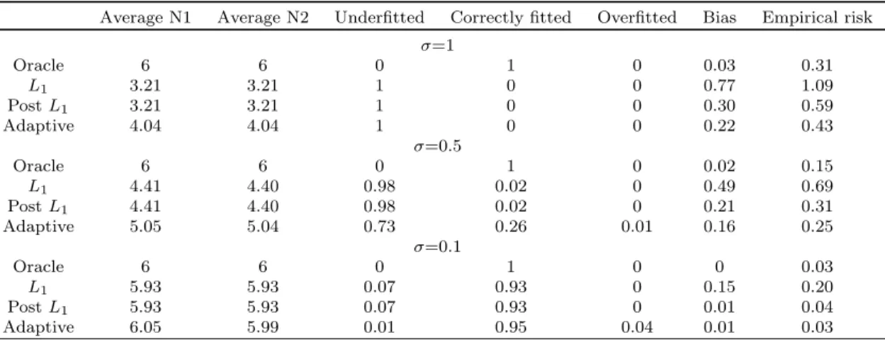
Table 2.1: Simulation results for model 1
Average N1 Average N2 Underfitted Correctly fitted Overfitted Bias Empirical risk
σ=1 Oracle 6 6 0 1 0 0.03 0.31 L1 3.21 3.21 1 0 0 0.77 1.09 PostL1 3.21 3.21 1 0 0 0.30 0.59 Adaptive 4.04 4.04 1 0 0 0.22 0.43 σ=0.5 Oracle 6 6 0 1 0 0.02 0.15 L1 4.41 4.40 0.98 0.02 0 0.49 0.69 PostL1 4.41 4.40 0.98 0.02 0 0.21 0.31 Adaptive 5.05 5.04 0.73 0.26 0.01 0.16 0.25 σ=0.1 Oracle 6 6 0 1 0 0 0.03 L1 5.93 5.93 0.07 0.93 0 0.15 0.20 PostL1 5.93 5.93 0.07 0.93 0 0.01 0.04 Adaptive 6.05 5.99 0.01 0.95 0.04 0.01 0.03
number of covariates selected by each estimator ˆβ, N2: the correct number of covariates selected by each estimaor, and the percentage of underfitted, correctly fitted, and overfitted. We evaluate the estimation accuracy by computing the norm of the bias and the empirical risk [E[xTi( ˆβ−β)]2]1/2. The results are summarized in the Table 1. We can see that although the proposed estimator may
still fail to select some significant variables whenσ is large due to the ultra-high dimensionality, it significantly improves the performance of quantile regression in both model selection and estimation, compared with theL1 penalized , postL1 penalized quantile estimators. Notice that the proposed
estimator does not necessarily treat 0 as an absorbing status even when the initial L1 penalized
estimator provides a zero estimate. This is the advantage of usingωj=|β˜|−1∧
√
n, which provides another opportunity to select the significant regressors, and hence provides better results.
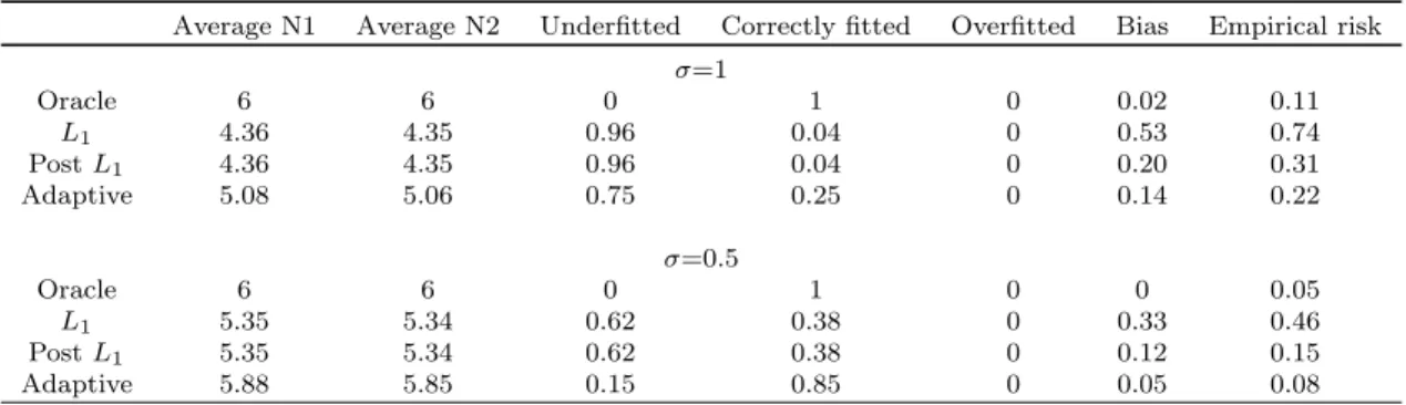
Following Wanget. al(2012), we consider model 2, which is a heterogenous version model 1.
yi=xTi β+ Φ(xi2)
where Φ(·) is the standard normal cumulative density function. We consider σ = 1 and σ= 0.5. And the results are presented in Table 2. Similar conclusions can be drawn from Table 2. All three
Table 2.2: Simulation results for model 2
Average N1 Average N2 Underfitted Correctly fitted Overfitted Bias Empirical risk
σ=1 Oracle 6 6 0 1 0 0.02 0.11 L1 4.36 4.35 0.96 0.04 0 0.53 0.74 PostL1 4.36 4.35 0.96 0.04 0 0.20 0.31 Adaptive 5.08 5.06 0.75 0.25 0 0.14 0.22 σ=0.5 Oracle 6 6 0 1 0 0 0.05 L1 5.35 5.34 0.62 0.38 0 0.33 0.46 PostL1 5.35 5.34 0.62 0.38 0 0.12 0.15 Adaptive 5.88 5.85 0.15 0.85 0 0.05 0.08
methods are able to work for regression models with heterogenous errors. However, as observed from Table 2, the adaptive penalized quantile regression drastically outperformed theL1 penalized , post
L1 penalized quantile estimators in both model selection and estimation.
2.5
Conclusion
In this chapter, the adaptive L1 quantile regression is introduced and studied for
high-dimensional sparse models. It is shown that such an adaptive robust estimator enjoys the oracle properties. In the case of quantile regression we can relax the moment conditions and the constant variance assumption on the error sequence from those used to prove oracle properties of penalized least squares loss methods for high-dimensional data. Our simulation results demonstrate that the
proposed estimator owns satisfactory finite sample performances. Although the oracle properties of a single quantile indexτ are presented here, the result can be easily extended to a finite composite quantile regression [Zou and Yuan (2008)].
Chapter 3
Adaptively Weighted Kernel
Regression
In this chapter, we develop a new kernel-based local polynomial methodology for nonpara-metric regression based on optimizing a linear combination of several loss functions. Optimal weights for least squares and quantile loss functions can be chosen to provide maximum efficiency and these optimal weights can be estimated from data. The resulting estimators are at least as efficient as those provided by existing procedures, but can be much more efficient for many distributions. The data based weights adapt to the tails of the error distribution resulting in a procedure which is both robust and resistant. Furthermore, the assumption of homogeneous error variance is not required. The method is used to model the change of global temperature anomolies over the last 100 years.
3.1
Introduction
Consider a general nonparametric model
Y =m(X) +σ(X), (3.1)
where Y is the response variable, X is the explanatory variable, m(·) is a smooth nonparametric regression function,σ(X) is a smooth function and is random error with a p.d.f. symmetric of 0. Without loss of generality, we assumeE[2
Various methods have been developed to fit this type of model [see e.g. Watson (1964); Wahba (1990); Fan and Gijbels (1996)]. It is fairly common to fit the model weighted least squares (LS) with local polynomial approximation [e.g. Fan and Gijbels (1992)]. However, least squares fitting can be very sensitive to heavy-tailed errors and severe outliers. Consequently least squares based local polynomial regression could fail to produce reliable estimates in some cases. In contrast, quantile regression [Koenker and Bassett (1978)] is robust against outliers, can provide a more complete model of the relationship between predictors and response variables [e.g. Koenker (2005)], owns excellent computational properties. [e.g. Portnoy and Koenker (1997)], and has widespread
applications [e.g. Yu et.al. (2003); Chernozhukov (2005)]. As a result, a substantial amount of
literature has been devoted to study local polynomial quantile regression [see e.g. Fanet al. (1994); Welsh (1996); Yu and Jones (1998)]. For some error structures, local polynomial quantile regression can be more efficient than local least squares polynomial regression. For example, if the error follows a Laplacian distribution, the local median polynomial regression has been demonstrated to be the most efficient [Fanet al. (1994); Welsh (1996); Yu and Jones (1998)]. In other cases, local quantile regression could be arbitrarily less efficient than local LS polynomial regression (e.g., for normal data), resulting from the fact that loss functions of quantile regressions penalize residuals of small magnitude too strongly.
To improve the performance of quantile regression, Koenker and Portnoy (1987) considered L-estimation for linear models. An L-estimator is a weighted average of quantile estimators, which can achieve high efficiency for non-normal data. Bickel (1973) and Koenker (1984) demonstrate that as the number of quantiles used increases, the optimally weighted L-estimator is as efficient
as the maximum likelihood estimator. However, it is difficult to find the optimal weights [see
Portnoy and Koenker (1989)], and the computational cost increases dramatically with the number of quantiles. Instead, Zou and Yuan (2008) introduced composite quantile regression (CQR), which equally weights quantile loss functions. Kaiet al. (2010) adapted composite quantiles to the local polynomial framework. They showed that the local polynomial CQR can significantly improve the estimation efficiency of its local LS counterpart for common non-normal errors. However, the loss in efficiency compared to the LS polynomial regression still exists in many scenarios. In addition to that, it is unclear how many quantiles should be used in the local polynomial CQR. Even for a huge data set, increasing the number of quantiles does not necessarily improve the efficiency of
least squares loss, these estimators can require a large number of quantiles to achieve efficiency
especially when the magnitude of errors is small. Bradic et al. (2011) attempted to minimize
composite loss functions simultaneously which results in a robust and efficient estimator for high dimensional linear regression.
In this chapter, we attempt to embed the usage of a convex combination of loss functions into nonparametric kernel regression to obtain a robust estimator with significant improvement in efficiency. Different from the combination of LS and least absolute deviation (LAD) for errors with finite errors or the combination of quantile losses for symmetric errors discussed in Bradic et al.
(2011), we combine the least squares loss with quantile loss functions for symmetric errors and picking weights to optimize asymptotic efficiency results in a method which inherits all strengths from least squares and quantile regression methods. We establish the asymptotic properties of the resulting estimator and show that it performs at least as well as the local LS polynomial estimator or a local polynomial CQR for any error distribution, and can improve the estimation efficiency for many distributions. Furthermore it achieves the same efficiency as the optimally weighted L-estimator
and can achieve higher efficiency than the equally weighted CQR of Kaiet al. (2010). We propose
a simple data-driven procedure to select weights for the convex combination and show that the aforementioned asymptotic properties can be achieved by this adaptively weighted local polynomial regression estimator. The adaptively weighted local polynomial estimator is quite robust and works well even if the error distribution does not have a finite variance.
The rest of this chapter is organized as follows. In Section 2, we define the adaptive weighted local polynomial regression estimator. In Section 3, we study theoretical properties of the proposed estimator. Section 4 presents our simulation studies and the analysis of a real data set. We give concluding remarks in Section 5, and relegate technical proofs to the Appendix B.
3.2
The adaptively weighted local polynomial regression
We start by setting up notations. Let ρτ(t) =τ1(t >0)t−(1−τ)1(t ≤0)t be the check function with quantile indexτ. Letτk =q+1k , k= 1,· · ·, qbe equally spaced quantile indices between
0 and 1. We denote the τkth quantile byqτk, k = 1,· · · , q. In particular, let τ0 = 0,qτ0 = 0 and
ρτ0(t) = t
2. We use F(·) andf(·) to denote the cumulative distribution function and probability
function. We also use the following notationsτk,k0 =τk∧k0−τkτk0 wherek∧k0 = min{k, k0}, and
τ0,k =E[i1(i≤qτk)], fork= 1,· · · , q.
In order to define the adaptively weighted local polynomial regression, let us briefly review the local LS polynomial regression, the local quantile polynomial regression and the local polynomial CQR.
Let (xi, yi) ben independently and identically distribution observations. Of interest is to estimate the value ofm(X) atx0. Suppose m(X) is smooth enough to be approximated by apth
order polynomial in a neighborhood of x0, that is, m(x) ≈ P
p j=0 1 j!m (j)(x 0)(x−x0)j. The local
LS polynomial regression estimator of (m(x0), m(1)(x0),· · · , m(p)(x0)) is defined as the minimizer
of the following objective function
min a0,a1,···,ap n X i=1 ρτ0 yi− p X j=0 1 j!aj(xi−x0) j K x i−x0 h (3.2)
where h is a smoothing parameter. Fan and Gijbels (1992) demonstrated that the local LS
poly-nomial regression owns several desirable properties: it adapts to a wide variety of design densities, significantly reduces bias at boundary points, and attains high minimax efficiency.
However, the local LS polynomial regression suffers from outliers and heavy-tailed errors.
Motivated by its robustness and other good features, several authors [Fan et al. (1994); Welsh
(1996); Yu and Jones (1998)] advocated local quantile polynomial regression
min a0,a1,···,ap n X i=1 ρτ yi− p X j=0 1 j!aj(xi−x0) j K x i−x0 h (3.3)
for some quantile index τ. Although the local quantile polynomial regression can be applied for
more general error structures, it can be arbitrarily inefficient compared to the local LS polynomial regression. To improve the efficiency of the local quantile polynomial regression while maintaining the robustness, Kaiet al. (2010) proposed the local polynomial CQR as follows
min a01,···,a0q,a1,···,ap n X i=1 q X k=1 ρτk yi−a0k− p X j=1 1 j!aj(xi−x0) j K x i−x0 h (3.4)
They showed that the local polynomial CQR can significantly improve efficiency compared to the local quantile polynomial regression. However, the loss of efficiency of the local polynomial CQR
still exists for some commonly seen distributions.
We consider combining CQR and LS to produce an efficient and robust regression estimator. Letθ= (a01,· · · , a0q, a0, a1,· · ·, ap) and denote the solution to the objective function
min θ n X i=1 q X k=0 βkρτk yi−a0k− p X j=0 1 j!aj(xi−x0) j K xi−x0 h (3.5)
by ˆθβ = (ˆa01,· · · ,ˆa0q,ˆa0,aˆ1,· · · ,ˆap). Here a00 = 0 and β0,· · · , βq are well-chosen non-negative weights which adapt to the error structures. The details about how to choose those weights are presented in Section 3.2. The adaptively weighted local polynomial regression estimator is defined as ˆ mβ(x0) = 1 2σ Pq k=1βkf(qτk)ˆa0k β0+21σ Pq k=1βkf(qτk)+ ˆa0 ˆ m(βj)(x0) = ˆaj, j= 1,· · · , p (3.6)
For identification purposes, we setσβ0+Pqk=1βkf(qτk)/2 = 1. The estimator becomes
ˆ mβ(x0) = 1 2 q X k=1 βkf(qτk)ˆa0k+ ˆa0. (3.7)
This formulation actually provides an advantage. In the following section, it can be seen that the variances of ˆm(x0) and ˆm(j)(x0), 1≤j ≤pare of similar forms. Consequently, minimizing them
separately still produces the same optimal weights vectorβ.
3.3
Asymptotic Properties
In this section, we state primitive regularity conditions and then establish the asymptotic properties of the adaptively weighted local polynomial regression estimator.
3.3.1
Regularity Conditions
To study the asymptotic properties of the adaptively weighted local polynomial regression estimator, the following regularity conditions are assumed throughout the rest of this paper. (A) m(·) has continuous (p+ 2)th derivative in the neighbourhood ofx0
(C) f is continuous and positive.
(D) gX(·) is positive and differentiable in the neighborhood ofx0.
(E) K(·) is a symmetric kernel function with a compact support [−M, M], and satisfies (a) |K(u)|< Ck (b) RM −MK(u)du= 1 (c) RM −Mu jK(u)du=µ j,R M −Mu jK2(u)du=ν
j,j≥0. In particular,µj =νj= 0 for oddj.
Regularity conditions A, C, D, E are commonly assumed in the literature [ see e.g. Fan (1992), Yu and Jones (1998), Kai et al. (2010)]. As is pointed out elsewhere, the assumption that K(·) has a compact support can be relaxed at the cost of more complicated technical proofs. In simulation studies, we exhibit the excellent performance of the proposed estimator with the classical normal
kernel. The assumption that f is symmetric about 0 is required in Kai et al. (2010). Although
weighted CQR for asymmetric errors was considered recently in Sunet al. (2013), we still maintain the symmetric assumption to simplify the complicated proof that the impact of the LS part is negligible when E[2
i] does not exist. However, our estimator can be generalized to asymmetric
distributions following Sunet al. (2013).
Up front, under the assumption thatE[2i]<∞, we establish the asymptotic properties of the adaptively weighted local polynomial regression estimator to demonstrate that it is more efficient and hence is favorable to other polynomial regression estimators. Next we considerE[2i] =∞and show that the impact of the LS part in the adaptively weighted local polynomial regression estimator is asymptotically negligible, while the efficiency is preserved under this infinite variance scenario. Therefore, the proposed estimator is a robust and efficient alternative to other polynomial regression estimators.
To avoid the complicated statements, we first illustrate our ideas via the i.i.d error models,
Y =m(X) +σ
3.3.2
Asymptotic Properties when
E
[
i]
2exists
Throughout this subsection we assume E[i]2 <∞. To state the asymptotic properties of the adaptively weighted local polynomial regression estimator, we need to introduce the following notations: Define S(β) = S11(β) S12(β) S21(β) S22(β)
whereS11(β) is aq×qdiagonal matrix with diagonal elementsβkf(qτk)/(2σ), fork= 1,· · ·, q,S22 is a (p+ 1)×(p+ 1) matrix with (j, j0)-entryµ(j+j0−2),forj, j0= 1,· · ·, p+ 1, andS12(β) =S21(β)T
is aq×(p+ 1) matrix with (k, j)-entryβkf(qτk)/(2σ)µj−1, fork= 1,· · · , q;j= 1,· · · , p+ 1. Let Vβ= 4β02σ 2−4β 0 q X k=1 βkστ0,k+ q X k,k0=1 βkβk0τk,k0, and we define Σ(β) = Σ11(β) Σ12(β) Σ21(β) Σ22(β)
where Σ11(β) is a q×q matrix with (k, k0)-entry βkβk0ν0τk,k0, for k, k0 = 1,· · · , q, Σ22(β) is a
(p+1)×(p+1) matrix with (j, j0)th elementV
βν(j+j0−2), forj, j0= 1,· · · , p+1, and Σ12(β) = ΣT21(β)
is aq×(p+ 1) matrix with (k, j)-entry (−2β0βkστ0,k+βkP q
k0=1βk0τk,k0)ν(j−1), fork= 1,· · · , q;j=
1,· · · ,(p+ 1).
Let ri,p = m(xi)−Ppj=0m(j)(x0)(xi −x0)j/j! be the residual of the Taylor expansion
of m(xi) at x0, and ξβ,i = −2β0(σi +ri,p) +Pqk=1βk[1(i ≤ (σqτk −ri,p)/σ)−τk]. We define
Wβ,n= (wβ,01,· · · , wβ,0q, wβ,0, wβ,1,· · ·, wβ,p)T, where wβ,0k =βk 1 √ nhn n X i=1 K xi−x0 hn [1 i ≤ σqτk−ri,p σ −τk], k= 1,· · ·, q wβ,j= 1 √ nhn n X i=1 K xi−x0 hn xi−x0 hn j ξβ,i, j= 0,· · · , p.
Then the asymptotic properties of the adaptively weighted local polynomial regression es-timator can be established in the following theorem:
E[2i]<∞. Ifhn→0 andnhn → ∞, then for any nonnegative weights vectorβ= (β0,· · ·, βq)T, p nhnS(β)Ahn(ˆθβ−θ∗) + 1 2g(x0) E[Wβ,n] L →N 0, 1 4g(x0) Σ(β) whereθ∗= (qτ1,· · ·, qτq, m(x0), m (1)(x
0),· · ·, m(p)(x0))T is a vector of true parameters andAhn is
a(q+ 1 +p)×(q+ 1 +p)diagonal matrix with diagonal elements(1,· · · ,1, h0
n/0!,· · ·, hpn/p!).
As special cases, two corollaries follow immediately.
Corollary 3.3.1 Under the same assumptions as Theorem 3.1, ifp= 1, we have
p nhn ˆ mβ(x0)−m(x0)− m(2)(x 0) 2 µ2h 2 n L →N 0, ν0σ 2 4g(x0) Vβ
and the mean squared error ofmˆ(x0)is
MSE( ˆmβ(x0)) = m(2)(x 0) 2 µ2 2 h4n+ ν0σ 2 4g(x0) Vβ nhn +op h4n+ 1 nhn (3.8)
Corollary 3.3.2 Under the same assumptions as Theorem 3.1, ifp= 1, then
p nhn ˆ m(1)β (x0)−m(1)(x0)− m3(x 0) 6 + m(2)(x 0)g(1)(x0) 2g(x0) µ 4 µ2 h2n L →N 0, ν2σ 2 4g(x0)h2nµ22 Vβ and MSE( ˆm(1)β (x0)) = m(3)(x 0) 6 + m(2)(x 0)g(1)(x0) 2g(x0) 2µ2 4 µ2 2 h4n+ ν2σ 2 4g(x0)µ22 Vβ nh3 n +op h4n+ 1 nh3 n (3.9) if p= 2, then p nhn ˆ m(1)β (x0)−m(1)(x0)− m(3)(x0)µ4 6µ2 h2n L →N 0, ν2σ 2 4g(x0)h2nµ22 Vβ and MSE( ˆm(1)β (x0)) = m(3)(x 0) 6 2µ2 4 µ2 2 h4n+ ν2σ 2 4g(x0)µ22 Vβ nh3 n +op h4n+ 1 nh3 n (3.10)
Corollary 3.1 indicates that the bias of ˆm(x0) relies on β throughCβ, which is assumed to be 1
ˆ
m(x0) can be chosen by minimizingVβ:
βopt= argmin
β≥0,αTβ=1
Vβ (3.11)
whereα= (1, f(qτk)/(2σ),· · ·, f(qτq)/(2σ))T.
Remark 3.3.1 When q → ∞, if we set β0 = 0 and minimize Vβ with respect to β, the resulting
covariance matrix is the same as that of the nonparametric polynomial L-estimation with optimal weights. Therefore, the proposed method is also as efficient as the maximum likelihood, whenq→ ∞.
Noting that the mean squared error of ˆm(1)β (x0) only depends on β byVβ as well, then βopt is also
optimal for estimatingm(1)(x0). For most practical interests, estimatingm(x0) is the main focus.
However, it can be shown thatβopt is optimal for estimating allm(j)(x0) forj≤p.
Since equation (3.11) is a constrained quadratic minimization problem, the closed form solution for the optimal weights can be difficult to obtain. However, in some cases, optimal weights can be explicitly found. We provide several examples to show the availability of the optimal weights.
Example 3.3.1 Let q= 1, τ1 = 12 andp≥1. In other words, we consider the combination of LS
and LAD, then the optimal weights are
β0,opt= 0 if 4f(0)1−2−2f4(0)f(0)EE[|[i||] i|]+1<0, 1 if 4f(0)1−2−2f4(0)f(0)EE[|[i||] i|]+1>1, 1 σ 1−2f(0)E[|i|] 4f(0)2−4f(0)E[| i|]+1 otherwise. and β1,opt= 2(1−β0,opt) f(0)
Example 3.3.2 Ifi∼N(0, λ2), thenβ0,opt= 1andβk,opt= 0, for all1≤k≤q.
Example 3.3.3 If i ∼ Laplace(0, λ) and q is odd, then βl,opt = 2f(0) for l = (q+ 1)/2, and
β0,opt=βk,opt= 0, for allk6=l.
Both the local polynomial LS and the local polynomial CQR estimators are special cases of weighted local polynomial regression. Regardless of the error distribution, the efficiency achieved by choosing the theorectically optimal weights can be no less than that gained by either of those methods. Moreover, the proposed estimator can be more efficient than the local LS polynomial regression estimator and the local polynomial CQR for some distributions, as Example 3.1 and 3.2 demonstrate.
Theorem 2 in Kaiet al. (2010) indicates that as the number of quantiles increases, the asymptotic
relative efficiency between CQR and LS converges to 1. For the proposed weighted estimator,
increasing the number of quantiles does not impact the efficiency in this way, but can in fact improve the asymptotic efficiency of the estimator.
AlthoughVβ is typically unobservable, we can replace them with consistent estimators. Let ˜
ζi be residuals of a
√
nhn-consistent preliminary estimation, i = 1,· · · , n. For example, we could use the residuals from local polynomial median regression, or residuals from local polynomial CQR, or the residuals from local LS polynomial regression, if the error terms {i} have a finite second moment. We use the notation ˜T to denote the empirical estimate ofT by using ˜ζi, for some statistic
T. Then ˜Vβ = 4β02σ˜2−4β0P
q
k=1βkσ˜τ˜0,k+P q
k,k0=1βkβk0τk,k0, and we can obtain the practically
optimal weights vector
ˆ β= argmax β≥0,α˜Tβ=1 ˜ Vβ (3.12) where ˜α = (˜σ,12f˜(˜qτ1),· · ·, 1
2f˜(˜qτq))T. The consistency of ˆβ can easily be verified. We have the following corollary:
Corollary 3.3.3 Under the same assumptions as Theorem 3.1,
p nhnS(βopt)Ahn(ˆθβˆ−θ ∗) + 1 2g(x0) E[Wβopt,n] L →N 0, 1 4g(x0) Σ(βopt)
The proposed estimator, using ˆβ obtained from (3.12) does not suffer from any loss of efficiency. Notice that in ˜Vβ, qτk, τ0,k, and fqτk need to be estimated. Therefore, the number of
quantiles depends on the sample size. When the sample size is small we recommend using only a few quantiles to avoid the impact by introducing too many parameters. On the other hand, if the sample size is large, more quantiles should be adopted. In practice, the cross-validation, AIC, BIC type estimators can be applied to choose the number of quantiles.
3.3.3
Asymptotic properties when
E
[
2i]
does not exist
Since least squares may not provide reliable estimates when heavy-tailed errors or outliers appear, in this case one might use a weight of zero (β0= 0) for the LS part of objective function (3.5).
In practice we do not know if the variance is finite and we propose picking weights using a numerical solution to the constrained quadratic minimization problem (3.12). So ˆβ0 is not necessarily 0. We
would like to find out if the proposed estimator can still be applied. The following theorem answers the aforementioned question.
Theorem 3.3.2 Suppose assumptions A,B,C,D, and E are satisfied. Furthermore, we assumeE[2
i]
does not exist. If hn →0 andnhn → ∞, then
p nhnS(βopt)Ahn(ˆθβˆ−θ ∗) + 1 2g(x0) E[Wβopt,n] L →N 0, 1 4g(x0) Σ(βopt)
This theorem indicates that ˆβ0 converges to 0 fast enough to make the instability caused by LS
negligible. Theorem 3.2 coupled with Theorem 3.1 imply that the adaptively weighted local poly-nomial regression can be applied universally. It is a very safe alternative to other estimators. In addition, because ˆβ is chosen to adapt to different error distributions, the resulting local polynomial regression estimator is asymptotically more efficient than the local polynomial CQR. Those features make the proposed estimator very appealing in practice.
3.3.4
Heterogeneous errors
In the foregoing sections, we exhibit the desirable theoretical properties of the adaptive-ly weighted local poadaptive-lynomial regression estimator under the homogeneous model. An interesting question naturally arises: “Can this method be applied to regression problems of which the error sequences are heterogeneous?”
The essential idea of the proposed procedure is to use the residuals from some preliminary method to select approximately optimal weights for the different loss functions. If the error sequences are homogeneous, then all residuals can be employed to establish the error structure. On the other hand, if the errors are heterogeneous, residuals of observations with covariate values closer tox0, the
point of interest, should contribute more to the local error structure estimation. Hence we can use weighted residuals to estimate the local error structure atx0, where weights are assigned by a kernel
function. Take the uniform kernel as an illustration, asn→ ∞, the number of observations falling into [x0−hn, x0+hn] is of ordernhn. Therefore, the asymptotic efficiency should not be impacted by doing local error structure estimation. In practice, the pilot fit also provides initial bandwidths so that we can manipulate observations falling into the smoothing window to approximate the error structure locally.
Theorem 3.3.3 Under model (1), suppose assumptions A,B,C,D, and E are satisfied. Furthermore, if hn→0andnhn→ ∞, then p nhnS(βopt)Ahn(ˆθβˆ−θ ∗) + 1 2g(x0) E[Wβopt,n] L →N(0, 1 4g(x0) Σ(βopt))
whereβˆ is obtained from (12) by using weighted local residuals.
Notice for heterogeneous cases, Vβ varies at different x. However, it can be shown that for the theoretical optimal weightsβoptat differentx, (β1,opt,· · · , βq,opt)’s andσ(x)β0,opt’s are are constant.
Thus, the weights are smooth functions of x, and so are the resulting estimators. Those simple
relationships in fact facilitate our computation to obtain the optimal weights ˆβ at differentx. We can randomly select some points in the supportX, and calculate ˆβ at each point. Then we can first average obtained ( ˆβ1,opt,· · · ,βˆq,opt) as practically global optimal weights for quantiles. Moreover, we can acquire a basis taking an average of ˆβ0/σˆ(x)’s. For a givenx, the product of the basis and
a consistent estimate ofσ(x) yields optimal ˆβ0.
3.3.5
Bandwidth Selection
The performance of local polynomial regression estimators depends crucially on the
smooth-ing parameter h. Obtaining a good bandwidth is very important for the success of the adaptively
weighted local polynomial regression estimator. Given a weights vectorβ, the optimal bandwidth
in the sense of minimizing MSE( ˆmβ(x0)) is
hβ,opt(x0) = 1 (m(2)(x 0))2 ν0σ2(x0) 4g(x0)µ22 Vβ 15 n−15,
and the optimal bandwidth for the local linear regression estimator is
hLS(x0) = 1 (m(2)(x 0))2 ν0σ2(x0) g(x0)µ22 15 n−15. It follows that hβ,opt(x0) = V β 4 1/5 hLS(x0) (3.13)
As suggested in Kai et al. (2010), when E[2i] exists we can exploit this simple relationship to select the optimal bandwidth for the proposed estimator using existing bandwidth selectors for the
local linear estimator. When E[2i] does not exist, we can similarly select the bandwidth via the
relationship between the proposed estimator and the local LAD linear estimator. In both cases, we can inferVβ˜ from preliminary estimates.
3.4
Numerical Studies and Applications
In this section, we conduct a simulation study which evaluates the finite sample performance
of the adaptively weighted local polynomial regression estimator. We then apply the proposed
estimator to a real data set as a demonstration of its practical use.
3.4.1
Simulations
In our simulation studies, we adopt the settings used in Kaiet al. (2010). We consider two simulation models.
1. Y = sin(2X) + 2 exp(−16X2) + 0.5, where X∼N(0,1)
2. Y =Xsin(2πX) + (1/5 + cos(2πX)/10), whereX ∼U nif(0,1)
In each model, we consider various distributions for: N(0,1) and Unif(−1/2,1/2) represent light-tailed errors; Laplace(0,1) represents moderate-tailed errors; a t3-distribution represents
heavy-tailed errors; a mixture of two normal distributions 0.95N(0,1) + 0.05N(0, σ2) with σ = 3,10
represent errors with light and severe outliers, respectively; and Cauchy(0,1) represent distributions without finite second moments. They belong to the domain of attraction of some stable distribution, respectively. For each combination, we simulated 400 independent training data sets, each consisting of 200 observations.
Since heavy-tailed errors and contaminated data sets are taken into account in the studies, we use a local polynomial median regression as a safe preliminary fit to get a consistent estimator ˜Vβ forVβ. The local polynomial median regression can be conveniently obtained viaquantregpackage in R.
We compare the proposed method with the classical local linear estimator and the local polynomial CQR via evaluating the integrated mean squared errors (IMSE), which is a summation
of mean squared errors at L equally spaced grid points over the interval at which the regression
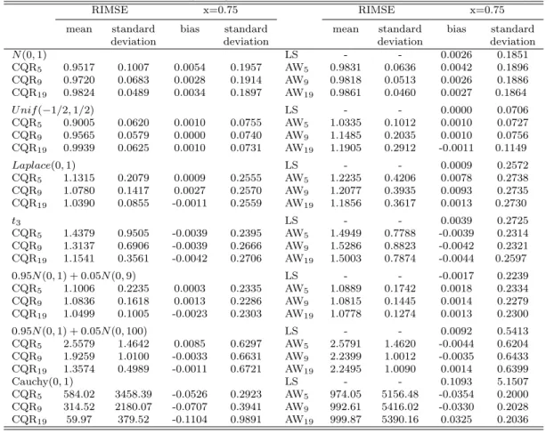
Table 3.1: Simulation results for model 1
RIMSE x=0.75 RIMSE x=0.75
mean standard bias standard mean standard bias standard deviation deviation deviation deviation
N(0,1) LS - - 0.0026 0.1851 CQR5 0.9517 0.1007 0.0054 0.1957 AW5 0.9831 0.0636 0.0042 0.1896 CQR9 0.9720 0.0683 0.0028 0.1914 AW9 0.9818 0.0513 0.0026 0.1886 CQR19 0.9824 0.0489 0.0034 0.1897 AW19 0.9861 0.0460 0.0027 0.1864 U nif(−1/2,1/2) LS - - 0.0000 0.0706 CQR5 0.9005 0.0620 0.0010 0.0755 AW5 1.0335 0.1012 0.0010 0.0727 CQR9 0.9565 0.0579 0.0000 0.0740 AW9 1.1485 0.2035 0.0010 0.0756 CQR19 0.9939 0.0625 0.0010 0.0731 AW19 1.1905 0.2912 -0.0011 0.1149 Laplace(0,1) LS - - 0.0009 0.2572 CQR5 1.1315 0.2079 0.0009 0.2555 AW5 1.2235 0.4206 0.0078 0.2738 CQR9 1.0780 0.1417 0.0027 0.2570 AW9 1.2077 0.3935 0.0093 0.2735 CQR19 1.0390 0.0855 -0.0011 0.2559 AW19 1.1856 0.3617 0.0013 0.2730 t3 LS - - 0.0039 0.2725 CQR5 1.4379 0.9505 -0.0039 0.2395 AW5 1.4949 0.7788 -0.0039 0.2314 CQR9 1.3137 0.6906 -0.0039 0.2666 AW9 1.5286 0.8823 -0.0042 0.2321 CQR19 1.1541 0.3561 -0.0042 0.2706 AW19 1.5003 0.7874 -0.0044 0.2597 0.95N(0,1) + 0.05N(0,9) LS - - -0.0017 0.2239 CQR5 1.1006 0.2235 0.0003 0.2335 AW5 1.0889 0.1742 0.0018 0.2334 CQR9 1.0836 0.1618 0.0013 0.2286 AW9 1.0815 0.1445 0.0014 0.2279 CQR19 1.0499 0.1005 -0.0023 0.2303 AW19 1.0778 0.1274 0.0013 0.2300 0.95N(0,1) + 0.05N(0,100) LS - - 0.0092 0.5413 CQR5 2.5579 1.4642 0.0085 0.6297 AW5 2.5791 1.4620 -0.0044 0.6204 CQR9 1.9259 1.0100 -0.0033 0.6631 AW9 2.2399 1.0012 -0.0035 0.6433 CQR19 1.3574 0.4989 -0.0011 0.6721 AW19 2.2495 1.0090 0.0014 0.6399 Cauchy(0,1) LS - - 0.1093 5.1507 CQR5 584.02 3458.39 -0.0526 0.2923 AW5 974.05 5156.48 -0.0354 0.2000 CQR9 314.52 2180.07 -0.0707 0.3941 AW9 992.61 5416.02 -0.0330 0.2028 CQR19 59.97 379.52 -0.1104 0.9891 AW19 999.87 5390.16 0.0325 0.2036
we estimatem(x) over [0,1] withL= 200. We considerq= 5,9,19 for the local polynomial CQR and the adaptively weighted local polynomial regression estimator. We use the normal kernel and select
hLS via a plug-in bandwidth selector, dpill, proposed by Ruppert et al(1995). For the proposed
estimator we select the bandwidth using equation (15). The bandwidths for CQR are calculated using their relationship to LS. We summarize our simulation results using RIMSE: the ratio of the IMSE of the local linear estimator over the IMSE of other estimators. We also evaluate the performance of the proposed estimator at a specific point. The results are presented in Table 1 and Table 2, where CQR5, CQR9, CQR19denote the local polynomial CQR withq= 5,9,19 respectively,
and likewise AW5, AW9, AW19denote the adaptively weighted local polynomial regression estimator
withq= 5,9,19, respectively.
It appears that the proposed method adapts well to the different error distributions. In Table 1 we can see that the adaptively weighted local polynomial regression estimators outperform LS and CQR counterparts for most of the distributions considered. The proposed estimator shows
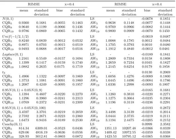
Table 3.2: Simulation results for model 2
RIMSE x=0.4 RIMSE x=0.4
mean standard bias standard mean standard bias standard deviation deviation deviation deviation
N(0,1) LS - - -0.0078 0.1851 CQR5 0.9360 0.1681 -0.0055 0.1463 AW5 0.9638 0.1148 -0.0077 0.1448 CQR9 0.9640 0.1199 -0.0066 0.1436 AW9 0.9769 0.0966 -0.0082 0.1444 CQR19 0.9786 0.0869 -0.0065 0.1432 AW19 0.9800 0.0909 -0.0070 0.1450 U nif(−1/2,1/2) LS - - -0.0019 0.0487 CQR5 0.8240 0.0839 -0.0012 0.0532 AW5 1.0088 0.1785 0.0012 0.0484 CQR9 0.8971 0.0703 -0.0015 0.0519 AW9 1.1705 0.3793 0.0010 0.0480 CQR19 0.9493 0.0688 -0.0017 0.0516 AW19 1.1912 0.4840 -0.0012 0.0481 Laplace(0,1) LS - - -0.0189 0.1841 CQR5 1.2161 0.5549 -0.0157 0.1694 AW5 1.2809 0.7334 0.0158 0.1808 CQR9 1.1399 0.1417 -0.0159 0.1740 AW9 1.2659 0.7234 0.0165 0.1827 CQR19 1.0882 0.2635 0.0175 0.1719 AW19 1.2145 0.6254 0.0179 0.1858 t3 LS - - 0.0130 0.2069 CQR5 1.4906 1.1322 -0.0097 0.1869 AW5 1.6056 1.4276 -0.0089 0.1800 CQR9 1.3753 1.1081 -0.0091 0.1860 AW9 1.6445 1.4496 -0.0084 0.1786 CQR19 1.2087 0.4249 -0.0095 0.1957 AW19 1.6336 1.2998 -0.0093 0.1807 0.95N(0,1) + 0.05N(0,9) LS - - -0.0165 0.1681 CQR5 1.1394 0.4607 -0.0220 0.2270 AW5 1.1260 0.3810 -0.0220 0.2271 CQR9 1.1296 0.3960 -0.0241 0.2313 AW9 1.1275 0.3664 -0.0235 0.2304 CQR19 1.0769 0.2372 -0.0231 0.2309 AW19 1.1196 0.3118 -0.0236 0.2291 0.95N(0,1) + 0.05N(0,100) LS - - -0.0193 0.2872 CQR5 3.4597 3.3701 -0.0219 0.2059 AW5 3.4498 3.3139 -0.0219 0.2014 CQR9 2.7592 2.2671 -0.0223 0.2360 AW9 3.0444 2.3735 -0.0219 0.2111 CQR19 1.6473 0.9416 -0.0189 0.2530 AW19 3.1194 2.4475 -0.0205 0.2152 Cauchy(0,1) LS - - 0.0999 2.3582 CQR5 814.34 6309.01 -0.0523 0.0436 AW5 1351.13 10207.48 -0.0366 0.0339 CQR9 629.06 4816.19 -0.0636 0.0556 AW9 1409.42 10972.55 -0.0359 0.0338 CQR19 328.93 3012.81 -0.0803 0.0872 AW19 1423.53 10795.12 -0.0365 0.0368
significant improvement over CQR in terms of RIMSE and also in terms of estimating the function at the pointx0= 0.75. The first section of Table 1 shows little loss in efficiency relative to LS, when
the error distribution is normal. Although the RIMSEs of the proposed estimators are slightly less than 1 for the normal distribution, the asymptotic ratio will get closer to 1 as sample sizes increase. The results in Table 2 indicate that the proposed adaptively weighted estimator still performs well in the presence of heteroskedasticity. In this case it appears that using too many quantiles can result in a loss of efficiency, but the proposed method tends to outperform CQR under the simulation set up.
3.4.2
A real data analysis
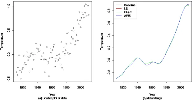
To illustrate its practical use, we apply the adaptively weighted local polynomial regression to the global temperature data set to study the modern temperature trend. The data set consist-ing of weighted global temperatures from 1911 to 2011 is available through U.S. national climatic data center (NCDC). Since the residuals from a local linear median regression have no significant autocorrelation according to the Ljung-Box test, the independence assumption of the error terms is not outlandish. We first use the local linear method, the local CQR and the proposed estimator
with 5 quantiles to fit the regression model. In the following analysis, we choose the local linear fit as the baseline fit. From Figure 3.1, we can see that all three procedures provide similar fits, and the local linear fit and the AW5 fit are almost identical. The interesting part is the right end of the
plots. It seems that the local linear fit and AW5 support the claim that the global temperature is
still increasing, while the CQR5 indicates there is a change point around 2010.
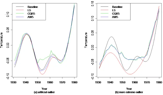
Although there is no outlier in the data set, we artificially create one to examine robustness properties, we move the observation of 1956 from -0.4431 to -0.6647. In Figure 3.2 (a) we only depict the fits from 1931 to 1980 , since for other years the outlier has no effect on the estimates. Comparing with Figure 3.1 (b), we note that the local CQR5 and AW5 still maintain similar patterns, while
the local linear estimator starts to deviate from the baseline. Moreover, we move the observation of 1956 from -0.4431 to -1.35 to simulate a severe outlier, and the fits are displayed in Figure 3.2 (b). Although all three procedures are affected by this severe outlier, the local linear changes drastically, whereas the local CQR5 and AW5are much less affected.
3.5
Conclusion
In this chapter, we combine the strength of the least squares and quantile regression to
propose the adaptively weighted local polynomial estimator for nonparametric regression. The
novelty of the method is that it adapts to the distribution of the error terms in a regression model. We have explicitly described how data can be used to select weights as well as the bandwidth parameter. It appears that even when the weights are selected from the data, the estimators perform nearly as well as the optimal choice. For example, if the distribution is normal the method is nearly as efficient as LS, but the method still works well if the errors follow at-distribution with 3 degrees of freedom. The estimators compete favorably with equally weighted composite quantile regression. The idea of weighting different objective functions and using asymptotic efficiency to select the optimal weights can be extended to other situations.
Appendix A
Proofs for Chapter 2
Appendix A-1: Consistency and sparsity
Define the score function of ρτ(·) by ϕτ(·), i.e. ϕτ(t) = τ1(t ≥ 0)−(1−τ)1(t < 0). ˆβτ is the minimizer of the objective function
Qτ(β) = n X i=1 ρτ(yi−xTiβ) +λn p X j=0 ωj|βj|
Throughout ˜β is a pn/(slog(n∨p))-consistent estimator ofβ∗.
Lemma A.1 Under assumptions A1-A5, ifλn/(
√
slog(n∨p))→ ∞andωi=|β˜τ j|−1for1≤j≤p,
then the adaptive L1 quantile regression estimatorβˆτ satisfiesβˆτ b= 0with probability tending to 1.
Proof: It can be seen that the objective functionQτ(β) is piecewise linear. According to Theorem 1 in Bloomfield and Steiger (1983, page 7), the minimum ofQτ(β) can be achieved at some breaking point ˘β, where ρτ(yi−xTi β˘) = 0 for some values ofi= 1,· · · , n.
Take the first derivative ofQ(β) at any differential point ˇβ ∈Rp+1 with respect toβj, j=
s+ 1,· · · , p, and we obtain that
∂Q(β) ∂βj |βˇ=− n X i=1 ϕ(yi−xTi βˇ)xij+λnωjsgn( ˇβj) (A.1) Let D( ˇβ, β∗) = n X i=1 ϕ(yi−xTiβˇ)xij− n X i=1 ϕ(yi−xTi β ∗)x ij
Note that, D( ˇβ, β∗) = X i≥q∗ xi,i≥q ∗ xi+x T i( ˇβ−β∗) [τ xij−τ xij] + X i≥qx∗i,i<qx∗i+xTi( ˇβ−β∗) [−(1−τ)xij−τ xij] + X i<qx∗i,i≥qx∗i+xTi( ˇβ−β∗) [τ xij+ (1−τ)xij] + X i<qx∗i,i<q∗xi+xTi( ˇβ−β∗) [−(1−τ)xij+ (1−τ)xij].
where qx∗i is the conditionalτth quantile ofi|xi. ForK1 ={i:q
∗ xi ≤i < q ∗ xi+x T i( ˇβ−β∗)} and K2={i:qx∗i > i≥q ∗ xi+x T i ( ˇβ−β∗)}, D( ˇβ, β∗) =−X K1 xij+ X K2 xij. Hence, | n X i=1 ϕ(yi−xTi βˇ)xij| =| n X i=1 ϕ(yi−xTi β∗)xij+D