Bayesian Multinomial Logistic Regression for
Author Identification
David Madigan
∗,†, Alexander Genkin
∗, David D. Lewis
∗∗and Dmitriy
Fradkin
∗,‡∗DIMACS, Rutgers University †Department of Statistics, Rutgers University
∗∗David D. Lewis Consulting
‡Department of Computer science, Rutgers University
Abstract. Motivated by high-dimensional applications in authorship atttribution, we describe a Bayesian multinomial logistic regression model together with an associated learning algorithm. Keywords: multinomial logistic regression, polytomous logistic regression, Bayesian estimation, classification, author identification, stylometry
PACS: 02.50.Sk;02.70.Rr;07.05.Kf;
INTRODUCTION
Feature-rich, 1-of-k authorship attribution requires a multiclass classification learning method and a scaleable implementation. The most popular methods for multiclass clas-sification in recent machine learning research are variants on support vector machines and boosting, sometimes combined with error-correcting code approaches. Rifkin and Klautau provide a review [12].
In this paper we focus on multinomial or polytomous generalizations of logistic regression. An important advantage of this approach is that it outputs an estimate of the probability that an object (documents in our application) belongs to each of the possible classes. Further, the Bayesian perspective on training a multinomial logistic regression model allows us to combine training data with prior domain knowledge.
MULTINOMIAL LOGISTIC REGRESSION
Let x=x1, ...,xj, ...,xdT be a vector of feature values characterizing a document to
be identified. We encode the fact that a document belongs to a class (e.g. an author) k∈ {1, ...,K}by aK-dimensional 0/1 valued vectory= (y1, ...,yK)T, whereyk=1 and
all other coordinates are 0.
Multinomial logistic regression is a conditional probability model of the form p(yk=1|x,B) = exp(β
T kx)
∑k0exp(βTk0x)
, (1)
parameterized by the matrixB= [β1, ...,βK]. Each column of B is a parameter vector
of binary logistic regression to the multiclass case.
Classification of a new observation is based on the vector of conditional probability estimates produced by the model. In this paper we simply assign the class with the highest conditional probability estimate:
ˆ
y(x) =argmax
k p(yk=1|x).
Consider a set of training examples D ={(x1,y1), . . .,(xi,yi), . . .,(xn,yn)}.
Maxi-mum likelihood estimation of the parametersBis equivalent to minimizing the negated log-likelihood: l(B|D) =−
∑
i "∑
k yikβT kxi−ln∑
k exp(βTkxi) # , (2)Since the probabilities must sum to one:∑kp(yk=1|x,B) =1, one of the vectorsβkcan
be set toβk=0without affecting the generality of the model.
As with any statistical model, we must avoid overfitting the training data for a multi-nomial logistic regression model to make accurate predictions on unseen data. One Bayesian approach for this is to use a prior distribution for Bthat assigns a high prob-ability that most entries of Bwill have values at or near 0. We now describe two such priors.
Perhaps the most widely used Bayesian approach to the logistic regression model is to impose a univariate Gaussian prior with mean 0 and varianceσ2
k j on each parameter βk j: p(βk j|σk j) =N(0,σk j) =√ 1 2πσk jexp( −βk j2 2σ2 k j ). (3)
Small values ofσk jrepresents a prior belief thatβk j is close to zero. We assumea priori that the components ofBare independent and hence the overall prior forBis the product of the priors for its components. Finding the maximuma posteriori(MAP) estimate of B with this prior is equivalent to ridge regression (Hoerl and Kennard, 1970) for the multinomial logistic model. The MAP estimate ofBis found by minimizing:
lridge(B|D) =l(B|D) +σ12 k j
∑
j∑
kβ2
k j. (4)
Ridge logistic regression has been widely used in text categorization, see for example [18, 10, 17]. The Gaussian prior, while favoring values of βk j near 0, does not favor them being exactly equal to 0. Since multinomial logistic regression models for author identification can easily have millions of parameters, such dense parameter estimates could lead to inefficient classifiers.
However, sparse parameter estimates can be achieved in the Bayesian framework remarkably easily if we use double exponential (Laplace) prior distribution on theβk j:
p(βk j|λk j) = λk j
As before, the prior forBis the product of the priors for its components. For typical data sets and choices of λ’s, most parameters in the MAP estimate forB will be zero. The MAP estimate minimizes:
llasso(B|D) =l(B|D) +λk j
∑
j∑
k |βk j|. (6)
Tibshirani [15] was the first to suggest Laplace priors in the regression context. Subse-quently, the use of constraints or penalties based on the absolute values of coefficients has been used to achieve sparseness in a variety of data fitting tasks (see, for example, [3, 4, 6, 16, 14]), including multinomial logistic regression [9].
Algorithmic approaches to multinomial logistic regression
Several of the largest scale studies have occurred in computational linguistics, where the maximum entropy approach to language processing leads to multinomial logistic regression models. Malouf [11] studied parsing, text chunking, and sentence extraction problems with very large numbers of classes (up to 8.6 million) and sparse inputs (with up to 260,000 features). He found that for the largest problem a limited memory Quasi-Newton method was 8 times faster than the second best method, a Polak-Ribere-Positive version of conjugate gradient. Sha and Pereira [13] studied a very large noun phrase chunking problem (3 classes, and 820,000 to 3.8 million features) and found limited-memory BFGS (with 3-10 pairs of previous gradients and updates saved) and preconditioned conjugate gradient performed similarly, and much better than iterative scaling or plain conjugate gradient. They used a Gaussian penalty on the loglikelihood. Goodman [7] studied large language modeling, grammar checking, and collaborative filtering problems using an exponential prior. He claimed not find a consistent advantage for conjugate gradient over iterative scaling, though experimental details are not given.
Krishnapuram, Hartemink, Carin, and Figueiredo [9] experimented on small, dense classification problems from the Irvine archive using multinomial logistic regression with an L1 penalty (equivalent to a Laplace prior). They claimed a cyclic coordinate
descent method beat conjugate gradient by orders of magnitude but provided no quanti-tative data.
We base our work here on a cyclic coordinate descent algorithm for binary ridge logistic regression by Zhang and Oles [18]. In previous work we modified this algorithm for binary lasso logistic regression and found it fast and easy to implement [5]. A similar algorithm has been developed by Shevade and Keerthi [14].
Coordinate decent algorithm
Here we further modify the binary logistic algorithm we have used [5] to apply to ridge and lasso multinomial logistic regression. Note that both objectives (4) and (6) are convex, and (4) is also smooth, but (6) does not have a derivative at 0; we’ll need to take special care with it.
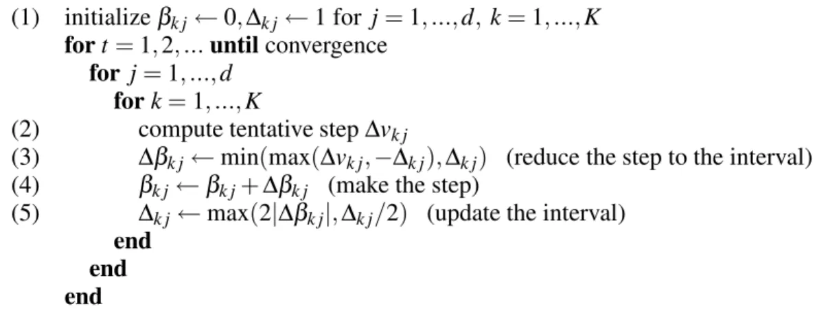
(1) initializeβk j←0,∆k j←1 for j=1, ...,d, k=1, ...,K
fort=1,2, ...untilconvergence
for j=1, ...,d
fork=1, ...,K
(2) compute tentative step∆vk j
(3) ∆βk j←min(max(∆vk j,−∆k j),∆k j) (reduce the step to the interval)
(4) βk j←βk j+∆βk j (make the step)
(5) ∆k j←max(2|∆βk j|,∆k j/2) (update the interval)
end end end
FIGURE 1. Generic coordinate decent algorithm for fitting Bayesian multinomial logistic regression.
The idea in the smooth case is to construct an upper bound on the second derivative of the objective on an interval around the current value; since the objective is convex, this will give rise to the quadratic upper bound on the objective itself on that interval. Min-imizing this bound on the interval gives one step of the algorithm with the guaranteed decrease in the objective.
Let Q(βk j(0),∆k j) be an upper bound on the second partial derivative of the negated
loglikelihood (2) with respect to βk j in a neighborhood ofβk j’s current valueβk j(0), so that: Q(βk j(0),∆k j)≥ ∂ 2l(B|D) ∂β2 k j for allβk j∈[βk j(0)−∆k j,βk j(0)+∆k j].
In our implementation we use the least upper bound (the inference is straightforward and the formula is omitted for the lack of space). Using Q we can upper bound the ridge objective (4) by a quadratic function ofβk j. The minimum of this function will be located atβk j(0)+∆vk jwhere
∆vk j= −
∂l(B|D)
∂βk j −2βk j(0)/σk j2
Q(βk j(0),∆k j) +2/σk j2 . (7)
Replacingβk j(0) withβk j(0)+∆vk j is guaranteed to reduce the objective only if∆vk j falls
inside the trust region[βk j(0)−∆k j,βk j(0)+∆k j]. If not, then taking a step of size∆k j in the
same direction will instead reduce the objective.
The algorithm in its general form is presented in Figure 1. The solution to the ridge regression formulation is found by using (7) to compute the tentative step at Step 2 of the algorithm. The size of the approximating interval ∆k j is critical for the speed of
convergence: using small intervals will limit the size of the step, while having large intervals will result in loose bounds. We therefore update the width, ∆k j, of the trust
The lasso case is slightly more complicated because the objective (6) is not differen-tiable at 0. However, as long asβk j(0)6=0, we can compute:
∆vk j=
−∂l(∂βk jB|D)−λk js
Q(βk j(0),∆k j) , (8)
wheres=sign(βk j(0)). We use∆vk jas our tentative step size, but in this case must reduce
the step size so that the new βk j is neither outside the trust region, nor of different sign thanβk j(0)). If the sign would otherwise change, we instead setβk j to 0. The case where
the starting value βk j(0)) is already 0 must also be handled specially. We must compute
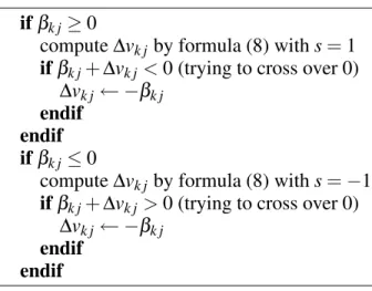
positive and negative steps separately using right-hand and left-hand derivatives, and see if either gives a decrease in the objective. Due to convexity, a decrease will occur in at most one direction. If there is no decrease in either direction βk j stays at 0. Figure 2 presents the algorithm for computing∆vk j in the Step 2 of the algorithm in Figure 1 for
the lasso regression case.
Software implementing this algorithm has been made publicly available1. It scales up
to 100’s of classes, 100,000’s of features and/or observations. ifβk j≥0
compute∆vk j by formula (8) withs=1
ifβk j+∆vk j<0 (trying to cross over 0)
∆vk j← −βk j
endif endif ifβk j≤0
compute∆vk j by formula (8) withs=−1
ifβk j+∆vk j>0 (trying to cross over 0)
∆vk j← −βk j
endif endif
FIGURE 2. Algorithm for computing tentative step of lasso multinomial logistic regression: replace-ment for Step 2 in algorithm Fig. 1.
Strategies for choosing the upper bound
A very similar coordinate descent algorithm for fitting lasso multinomial logistic re-gression models has been presented by Krishnapuram, Hartemink, Carin, and Figueiredo
[9]. They use the following bound on the Hessian of the negated loglikelihood [1]: H≤
∑
i 1 2 h I−11T/Ki⊗xixiT, (9)whereHis thedK×dKHessian matrix; Iis theK×K identity matrix;1is a vector of 1’s of dimension K; ⊗ is the Kronecker matrix product; and matrix inequality A≤B
meansA−Bis negative semi-definite.
For a coordinate descent algorithm we only care about the diagonal elements of the Hessian. The bound (9) implies the following bound on those diagonal elements:
∂2l(B|D) ∂β2
k j ≤
K−1
2K
∑
i x2i j. (10) the tentative updates for ridge and lasso case can now be obtained by substituting right-hand side of (10) instead of Q(βk j(0),∆k j) into (7) and (8). Note that it does not reallydepend onbeta(0)k j ! As before, a lasso update that would cause aβk jto change sign must be reduced so thatβk jinstead becomes 0.
In contrast to our boundQ(βjk,∆jk), this one does not need to be recomputed whenB
changes, and no trust region is needed. On the downside, it is a much looser bound than Q(βjk,∆jk).
EXPERIMENTS IN ONE-OF-K AUTHOR IDENTIFICATION
Data sets
Our first data set draws from RCV1-v22, a text categorization test collection based on
data released by Reuters, Ltd.3. We selected all authors who had 200 or more stories each
in the whole collection. The collection contained 114 such authors, who wrote 27,342 stories in total. We split these data randomly into training (75% - 20,498 documents) and test (25% - 6,844 documents) sets.
The other data sets for this research were produced from the archives of several listserv discussion groups on diverse topics. Different groups included from 224 to 9842 postings and from 23 to 298 authors. Each group was split randomly: 75% of all postings for training, 25% for test.
The same representations were used with all data sets, and are listed in Figure 3. Feature set sizes ranged from 10 to 133,717 features. The forms of postprocessing are indicated in the name of each representation:
• noname: tokens appearing on a list of common first and last names were discarded before any other processing.
2http://www.ai.mit.edu/projects/jmlr/papers/volume5/lewis04a/lyrl2004_rcv1v2_README.htm 3http://about.reuters.com/researchandstandards/corpus/
• Dpref: only the firstDcharacters of each word were used. • Dsuff: only the lastDcharacters of each word were used.
• ˜POS: some portion of each word, concatenated with its part-of-speech tag was used.
• DgramPOS: all consecutive sequences ofDpart-of-speech tags are used.
• BOW: all and only the word portion was used (BOW = “bag of words”). There are also two special subsets defined of BOW. ArgamonFW is a set of function words used in a previous author identification study [8]. The set briansis a set of words automatically extracted from a web page about common errors in English usage4.
Finally, CorneyAll is based on a large set of stylometric characteristics of text from the authorship attribution literature gathered and used by Corney [2]. It includes features derived from word and character distributions, and frequencies of function words, as listed inArgamonFW.
Results
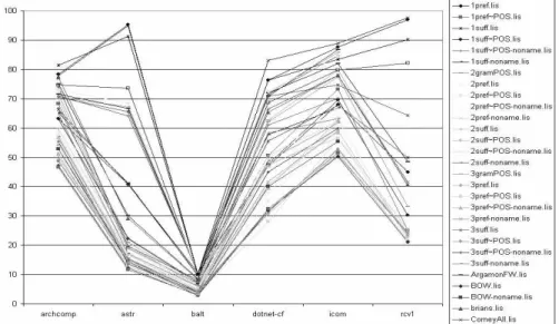
We used Bayesian multinomial logistic regression with Laplace prior to build classi-fiers on several data sets with different representations. The performance of these clas-sifiers on the test sets is presented in Figure 3.
One can see that error rates vary widely between data sets and representations; however the lines that correspond to representations do not have very many crossings between them. If we were to order all representations by the error rate produced by the model for each data set, the order will be fairy stable across different data sets. For instance, representation with all words ("bag-of-words", denoted BOW in the chart) almost always results in the lowest error rate, while pairs of consecutive part of speech tags (2gramPOS in the chart) always produces one of the highest error rates. There are some more crossings between representation lines near the right-most column that reflects RCV1, hinting that this data set is essentially different from all listserv groups. Indeed, RCV1 stories are produced by professional writers in the corporate environment, while the postings in the discussion groups are written by people in an uncontrolled environment on topic of their interest.
The National Science Foundation funded this work through the Knowledge Discovery and Dissemination (KD-D) program.
REFERENCES
1. D. Böhning. Multinomial logistic regression algorithm. Annals of the Institute of Statistical Mathe-matics, 44(9):197–200, 1992.
2. M. Corney. Analysing e-mail text authorship for forensic purposes. master of information technology (research) thesis, 2003.
FIGURE 3. Test set error rates on different data sets with different representations.
3. B. Efron, T. Hastie, I. Johnstone, and R. Tibshirani. Least angle regression.Ann. Statist., 32(2):407– 499, 2004.
4. M. A. T. Figueiredo. Adaptive sparseness for supervised learning. IEEE Transactions on Pattern Analysis and Machine Intelligence, 25(9):1150–1159, 2003.
5. A. Genkin, D. D. Lewis, and D. Madigan. Large-scale bayesian logistic regression for text catego-rization., 2004.
6. F. Girosi. An equivlance between sparse approximation and support vector machines. Neural Computation, 10:1445–1480, 1998.
7. J. Goodman. Exponential priors for maximum entropy models. InProceedings of the Human Lan-guage Technology Conference of the North American Chapter of the Association for Computational Linguistics: HLT-NAACL 2004, pages 305–312, 2004.
8. M. Koppel, S. Argamon, and A. R. Shimoni. Automatically categorizing written texts by author gender.Literary and Linguistic Computing, 17(4), 2003.
9. B. Krishnapuram, A. J. Hartemink, L. Carin, and M. A. T. Figueiredo. Sparse multinomial logistic regression: Fast algorithms and generalized bounds. IEEE Trans. Pattern Anal. Mach. Intell., 27(6):957–968, 2005.
10. F. Li and Y. Yang. A loss function analysis for classification methods in text categorization. InThe Twentith International Conference on Machine Learning (ICML’03), pages 472–479, 2003. 11. R. Malouf. A comparison of algorithms for maximum entropy parameter estimation. InProceedings
of the Sixth Conference on Natural Language Learning (CoNLL-2002)., pages 49–55, 2002. 12. R. M. Rifkin and A. Klautau. In defense of one-vs-all classification. Journal of Machine Learning
Research, 5:101–141, 2004.
13. F. Sha and F. Pereira. Shallow parsing with conditional random fields, 2003.
14. S. K. Shevade and S. S. Keerthi. A simple and efficient algorithm for gene selection using sparse logistic regression.Bioinformatics, 19:2246–2253, 2003.
15. R. Tibshirani. Regression shrinkage and selection via the lasso. Journal of the Royal Statistical Society (Series B), 58:267–288, 1996.
16. M. Tipping. Sparse bayesian learning and the relevance vector machine. Journal of Machine Learning Research, 1:211–244, June 2001.
17. J. Zhang and Y. Yang. Robustness of regularized linear classification methods in text categorization. InProceedings of SIGIR 2003: The Twenty-Sixth Annual International ACM SIGIR Conference on Research and Development in Information Retrieval, pages 190–197, 2003.
18. T. Zhang and F. Oles. Text categorization based on regularized linear classifiers. Information Retrieval, 4(1):5–31, April 2001.