Variance Risk Premia in Commodity
Markets
*Marcel Prokopczuk
,and Chardin Wese Simen
§First version: January 04, 2013
This Version: March 10, 2014
Abstract
We use a large panel of commodity option prices to study the market price of variance risk. We construct synthetic variance swaps and find significantly negative variance risk premia in nearly all commodity markets. An equally-weighted portfolio of short commodity variance swaps earns an annualized Sharpe Ratio of around 40 %. We document increasing comovements across bonds, commodities and equity variance swap returns, suggesting that the variance swap markets are increasingly integrated. Finally, we show that commodity variance risk premia are distinct from price risk premia, indicating that variance risk is unspanned by commodity futures.
JEL classification: G12, G13
Keywords: Commodities, Variance risk premia, Variance swaps
*
Marcel Prokopczuk gratefully acknowledges financial support from the British Academy. We thank Jaime Casassus, Mathias Fengler (DGF discussant), Yuecheng Jia (FMA discussant), Steen Koekebakker, Pascal Maenhout, Frank Moraux (AFFI discussant), Gabriel J. Power (EFA discussant), Leonidas Rompolis (FMA discussant), Mark Shackleton, Natalia Sizova (WFA discussant), George Skiadopoulos, Lazaros Symeonidis, Stephen Taylor (EFMA discussant), Yingying Wu and seminar participants at the Commodity Finance Workshop (2012), University of Reading (2012), Zeppelin University (2012), Cornell–FDIC Derivative Securities and Risk Management Conference (2013), Eastern Finance Association (2013), European Financial Management Association (2013), Financial Management Association (2013), German Finance Association (2013), International French Finance Association (2013), University of Liverpool (2013) and Western Finance Association (2013) for helpful comments.
Zeppelin University, Am Seemooser Horn 20, 88045, Friedrichshafen, Germany. Contact: [email protected]
ICMA Centre, Henley Business School, University of Reading, RG6 6BA, UK §
University of Liverpool, Chatham Street, Liverpool, L69 7ZH, United Kingdom. Contact: [email protected]
I
Introduction
Over the past decade, commodity markets have witnessed tremendous increases in volatility. Given their role as consumption goods, factors of production and financial assets, managing commodity volatility is crucial for a wide number of market participants such as commercial hedgers and investors. Arguably, these developments have motivated the successful launch of commodity related volatility derivatives such as oil and gold VIX futures contracts. The rapid proliferation of these derivatives raises several questions. Chief among them include: how large is the compensation required by investors to bear variance risk in commodity markets?
To what degree are commodity variance risk premia time varying? Are there
commonalities in commodity variance risk premia? How do commodity variance risk premia relate to bond and equity variance risk premia? What is the relationship between price and variance risk premia? These are some of the questions we seek to answer.
In this paper, we comprehensively analyze the market price of variance risk in 21 commodity markets between 1989 and 2011, a period which includes the recent financial crisis. In doing so, we make three important contributions to the literature. First, we use a large panel of futures and options data to construct synthetic commodity variance swaps. This is important as commodity variance swaps allow us to estimate the market price of variance risk in a model-free way. Variance swaps are made up of a fixed leg, the variance swap rate, and a floating leg, the realized variance. Each day, we combine static positions in option contracts to replicate the variance swap rate. Next, we estimate the floating leg by computing the realized variance of the underlying commodity over the maturity of the variance swap. We then estimate commodity variance risk premia as the sample average of the difference between the floating and fixed legs of variance swaps (Carr and Wu, 2009; Driessen et al., 2009). Analyzing variance swaps that mature in 60 and 90 days, we find significant variance risk premia in 18 out of 21 commodity markets.1
1
Typically, commodity options have bimonthly or quarterly expiration cycles. As a result, we focus on variance swaps that mature in 60 and 90 days.
This is in contrast to the findings of Carr and Wu (2009) and Driessen et al. (2009), who find very limited evidence of variance risk premia in individual equities.2
Typically, commodity variance risk premia are negative and economically large. An equally-weighted portfolio of short commodity variance swaps yields an annualized Sharpe Ratio (40 %), which is of similar magnitude as that of a short position in the S&P 500 variance swap. Moreover, this Sharpe Ratio is four times larger than that of an equally-weighted portfolio of long commodity futures, underscoring the profitability of commodity variance swaps.
Our second novel contribution consists in providing the first analysis of commonalities in variance swap returns. Our investigation proceeds in three steps. First, we focus on comovements within commodity sectors. To achieve this goal, we group commodities into sectors, i.e. energy, grains, livestock, metals, tropical,
and wood. For each sector, we compute the average pair-wise correlation of
commodity variance swap returns. We find modest correlations between variance swap returns of similar commodities. For example, the average pair-wise correlation
among energy commodity variance swap returns is around 30 %. Second, we
investigate commonalities across sectors. For each commodity sector, we compute an equally-weighted portfolio of variance swap returns. We then study the comovement across distinct sectors and find correlation coefficients that are generally below 20 %. Third, we analyze how commodity variance swap returns correlate with bond (30-Year Treasury) and equity index (S&P 500) variance swap returns. Our results evidence modest (typically below 30 %) unconditional correlations across asset classes. Motivated by the literature on the financialization of commodity markets (Tang and Xiong, 2012), we partition our sample into two distinct subperiods. The first subperiod, which we label “pre-financialization”, ends in November 2004. The “financialization” period, which captures the period of increased investor flows in commodity markets, runs from December 2004 until the end of our sample. We confirm that variance risk is significantly priced during each of these subperiods.
2
Carr and Wu (2009) report significantly negative variance risk premia in 8 out of 35 individual equities only. Similarly, Driessen et al. (2009) find significant variance risk premia in 29 out of 127 individual stocks.
More importantly, we document increasing commonalities in variance swap returns across markets. The case of energy markets is particularly telling. Prior to December 2004, equity and energy variance swap returns are only weakly correlated, as evidenced by their low correlation coefficient (2.62 %). However, this correlation rises to around 48 % during the period of financialization. This finding indicates that the financialization of commodity markets affects not only the risk premia related to the first but also the second moment of commodity returns.
Our third contribution consists in investigating the relationship between
commodity variance risk premia on the one hand and equity, bond and commodity
price risk premia on the other. To do so, we follow a three-pronged approach. First, we examine the relationship between commodity variance risk premia and the determinants of equity risk premia. This is important because our findings of negative variance risk premia may be the result of a significantly negative correlation between innovations to commodity variance and equity risk factors. To investigate this, we regress commodity variance risk premia on the 3 factors of Fama and French (1993). We find that the slope estimates are not statistically distinguishable from zero, indicating that commodity variance risk premia are unrelated to the market risk premium. Furthermore, the regressions result in very low explanatory power, confirming that commodity variance risk premia are unrelated to the determinants of the equity risk premium. Second, we analyze the relationship between commodity variance risk premia and bond risk premia. We use the Cochrane and Piazzesi (2005) and Ludvigson and Ng (2009) factors as determinants of bond risk premia and regress commodity variance swap returns on these factors, obtaining significantly large intercepts and very low explanatory power. Typically, the coefficient estimates of the independent variables are statistically insignificant. In short, our results suggest that commodity variance risk premia are independent of bond risk premia. Finally, we analyze the link between the variance risk premium of a commodity and its price risk premium by regressing the former on the latter. Generally, our regression model yields very low explanatory power and mainly insignificant slope estimates. These results indicate that variance risk premia are largely orthogonal
to price risk premia. In other words, commodity variance risk is not spanned by commodity futures, suggesting that options contracts are non-redundant securities. We perform several checks to establish the robustness of our main results. First, we investigate whether expected (rather than realized) commodity variance risk premia are also significant. To this end, we use historical variance as a proxy for expected variance to compute the floating leg of variance swaps and repeat our investigation. We show that expected commodity variance risk premia are significantly negative, confirming that our main findings remain unchanged. We then investigate the robustness of our variance swap estimates. To begin with, we use a cubic spline (rather than linear) interpolation technique. Again, we obtain similar results. We also use different truncation points and find that they do not materially affect our main findings. Additionally, we assess the effect of jumps on the variance risk premia estimates and demonstrate that they do not change our main conclusions: there are significantly negative variance risk premia in commodity markets. Moreover, we show that our synthetic swap rates are highly correlated with publicly available indices. Relatedly, we show that our results are robust to concerns related to the tradability of commodity options. We also analyze the impact of seasonality on our main results. In a first step, we regress variance swap returns on twelve monthly dummies to purge out potential seasonal fluctuations. We then repeat our main analyses and find little differences with our baseline results. Finally, we use non-overlapping samples of variance swaps and obtain similar results, demonstrating that our results are robust to overlapping observation biases.
Our work is related to the literature on option trading returns. Coval and Shumway (2001), Bakshi and Kapadia (2003a), Bakshi and Kapadia (2003b), Carr and Wu (2009), Driessen et al. (2009), Trolle and Schwartz (2010), Wang et al. (2011) and Mueller et al. (2013), among others, study the market price of variance risk in a variety of financial markets and reach conflicting findings.3 This may be
3
For example, Bakshi and Kapadia (2003a) and Bakshi and Kapadia (2003b) use a delta-hedging approach and find significant volatility risk premia in individual equities. In contrast, Carr and Wu (2009) and Driessen et al. (2009) construct synthetic variance swaps and find little evidence of variance risk premia in individual equities.
due to their fairly short sample periods and different methodologies, which make the results difficult to compare and interpret. In contrast to them, we use a model-free approach to analyze the market price of variance risk over a long sample period in a large number of commodity markets. Covering a long time series is crucial in order to draw robust inferences about the time varying variance risk premia. Likewise, covering a large number of markets allows us to present the first study on commonalities in variance risk premia across assets.
Our paper is also connected to the literature on commodity futures risk premia. Gorton et al. (2013), Daskalaki et al. (2014) and Szymanowska et al. (2014), among others, study the characteristics of risk premia in commodity futures prices. We analyze a different type of risk premium. Specifically, we focus on the compensation that investors require for bearing variance (rather than price) risk in commodity
markets. We show that, contrary to price risk premia, commodity variance
risk premia are significantly negative and economically large. More importantly, commodity variance risk premia are largely orthogonal to price risk premia. This important result implies that variance risk is unspanned by commodity futures, making options contracts non-redundant securities.
We also contribute to studies on the integration of commodity markets with traditional asset classes. Recent works by Tang and Xiong (2012) and Singleton (2014) analyze the financialization of commodity markets and the effect of investor flows on the first moment of commodity returns. They show that commodity returns are increasingly integrated with returns on traditional asset classes. We complement this literature by documenting similar effects for the second moment of commodity returns: commodity variance swap returns are increasingly correlated with bond and equity variance swap returns. In short, our results provide direct and model-free evidence that the financialization of commodity markets is a pervasive phenomenon that affects both the futures and options markets.
This paper proceeds as follows. In Section II we introduce our methodology and describe the data set employed. In Section III we present and discuss the empirical results of our study. Finally, Section IV concludes.
II
Methodology and Data
A.
Methodology
Empirical studies on variance risk premia are usually anchored around one of the following three estimation approaches: parametric, semi-parametric or model-free. The parametric approach consists of specifying a data-generating process for
the underlying. In this framework, the variance risk premium is usually a
parameter to be estimated by exploiting information from the underlying and options prices. This approach is not only computationally intensive but also subject to specification errors since it explicitly assumes a specific data-generating process for the underlying. Consequently, parametric estimates of variance risk premia are joint tests of model specification and variance risk premia. Broadie et al. (2007) empirically examine the impact of model misspecification on risk premia. They conclude that the significance of variance risk premia depends crucially on assumptions about the presence of jumps in the data-generating process.4
Bakshi and Kapadia (2003a) propose to study variance risk premia in a semi-parametric manner by analyzing the profitability of delta-hedged at-the-money (ATM) straddles. This approach is motivated by financial theory, which argues that option prices are affected by changes in implied volatility and the underlying’s price. Since delta-neutral ATM straddles are insensitive to small movements of the underlying’s price, their profitability is mainly driven by changes in implied volatility. Hence, the profitability of delta-neutral ATM straddles may shed light on the existence of volatility risk premia. Though intuitive, this approach is still vulnerable to the criticism that it relies on a specific hedging model.
To overcome these problems, the more recent model-free approach builds on variance swaps defined as swap contracts in which the floating leg corresponds to the realized variance of the underlying over a predetermined period. The underlying idea is that unconditional variance risk premia are equal to the sample averages of
4
Pan (2002) reaches similar conclusions. She shows that once jumps are allowed for, the variance risk premium becomes insignificant in her data set.
variance swap pay-offs which are the differences between the realized variance and the risk-neutral expectation of variance. No-arbitrage arguments imply that the rate of a variance swap, SVt,T, must be equal to the risk-neutral expectation of variance,
EQt (Vt,T), over the life of the swap. Thus, the unconditional variance risk premium
can be estimated as the sample average of variance swap pay-offs. The pay-off to a variance swap contract (with a notional of 1) for the period ranging from t to T, V RPt,T, is given by:
V RPt,T =RVt,T −SVt,T (1)
where RVt,T denotes the realized variance between t and T under the physical
measure.
Consequently, quantifying variance risk premia reduces to estimating realized variance and variance swap rates. Whilst realized variance estimators have been extensively studied (see, e.g., Andersen et al. (2009) and the references therein), until recently, little has been known about the latter. In a seminal study, Britten-Jones and Neuberger (2000) elaborate a static replicating strategy to estimate the variance swap rate under the assumption that the underlying follows a continuous process.5
More precisely, they derive the following relationship:
EQt (Vt,T) =M F IVt,T = 2ert(T−t) T −t " Z Ft,T 0 P(t, K, T) K2 dK+ Z +∞ Ft,T C(t, K, T) K2 dK # (2) where EQt(Vt,T) and M F IVt,T refer to the risk-neutral expectation of variance and
model-free implied variance between t and T, respectively. The annualized risk-free rate is denoted by rt. Ft,T denotes the futures contract observed at time t and
expiring atT. P(t, K, T) andC(t, K, T) denote the price at timet of European put and call options struck at K and expiring atT.
Subsequently, Jiang and Tian (2005) extend this approach to a broader class of models by formally showing that Equation (2) holds for jump diffusion processes
5
as well.6 This result leads to the conclusion that the variance swap approach for
estimating variance risk premia is essentially model-free in the sense that it holds for a general class of data-generating processes.
Therefore, we employ a methodology that is similar to that of Carr and Wu (2009). Assume we want to synthetically create a 60 day variance swap. On each trading day, we obtain and sort all out-of-the-money (OTM) options by time to maturity. We identify the two maturities T1 andT2 that are closest to and cover 60
days. We retain options of maturities T1 and T2 only. We require the existence of at
least two OTM put and two OTM call options for each of the two maturities. We exclude from our sample all trading days that do not meet this requirement. As in Trolle and Schwartz (2010), we truncate the first and second integrals in Equation (2) at Kl and Ku respectively:
Kl = Ft,T exp
−10σT
(3)
Ku = Ft,T exp10σT (4)
where Kl and Ku refer to the lower and higher truncated strikes. Ft,T refers to
the futures contract observed at time t and expiring at T,σ is the average implied
volatility of all OTM options and T denotes the time to maturity of the option
contract.7 For each maturity, we linearly interpolate available Black (1976) implied
volatilities across moneyness.8 For strikes higher (lower) than the highest (lowest)
listed strike price but lower (higher) than Ku (Kl), we assume constant implied
volatility. Pursuing this approach, we obtain a grid of 1,000 equidistant implied volatilities for strikes between Ku and Kl.
We then convert implied volatilities back into European option prices using the Black (1976) option pricing formula. We evaluate the integrands at each of the 1,000 points and numerically approximate (trapezoidal rule) the integrals in Equation (2)
6
Although jumps introduce errors in the replicating strategy, the numerical analysis of Carr and Wu (2009) indicates that these biases are negligible. We use a recent result by Rompolis and Tzavalis (2013) to analyze the effect of jumps on our main results. As Section E.4 shows, our findings are robust to the impact of jumps.
7
Our results are robust to the choice of truncation points. See SectionE.3 for further details.
8
to estimate the variance swap rate. Finally, we linearly interpolate between the two swap rates to obtain the 60 day variance swap rate. We repeat the above steps every day to obtain time series of 60 day variance swap rates.
As is common in empirical studies, we estimate realized variance as follows:
RVt,T = 252 T −t T X i=t+1 log Fi,T Fi−1,T 2 (5)
whereT is the maturity date of the variance swap, Fi,T denotes the futures contract
observed at time i and expiring at time T.
Note that, contrary to individual equities, commodity options are written on futures contracts which life span is finite. As a result, the time series of the first nearby contract could exhibit spikes at rollover dates especially in markets characterized by steep term-structure of futures. Given that these spikes could bias our estimates of realized variance upward, we construct a constant maturity futures time series by linear interpolation of futures contracts maturing at T1 and T2.
B.
Data
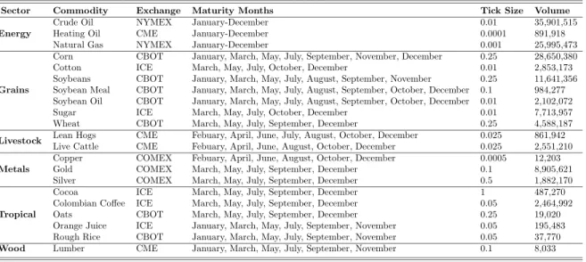
We obtain our futures and option data set from the Commodity Research Bureau (CRB). The data set contains information on the strike price, maturity and settlement price of individual commodity derivatives. Table 1 lists the 21 commodities included in our sample. To mitigate the effect of micro-structure related issues such as infrequent trading and stale prices, we only retain options with time-to-maturity of at least 12 days. We further delete options with prices lower than five times the minimum tick size reported in Table 1. Given that our data set comprises American options and that our estimation approach requires European option prices, we convert the American option prices into European prices by following the standard approach of Barone-Adesi and Whaley (1987).
Table 1 also reports the annual average volume of individual commodity options for the years 2010 and 2011. We collect the volume data from the monthly volume
report published on the exchange’s websites.9 Generally, we see cross-sectional
variation in trading activity with higher trading volume in some energy, grains and metal commodities than in other commodity sectors.
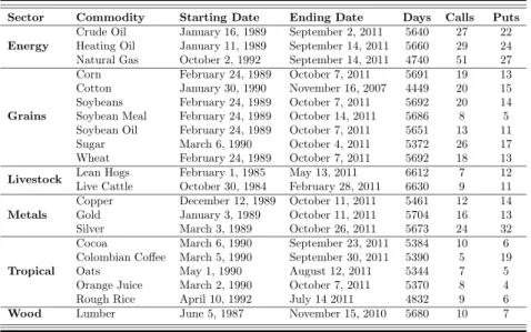
Our empirical analysis focuses on variance swaps with maturity of 60 and 90 days. This decision is motivated by the observation that, with the exception of energy markets, no other commodity exhibits a monthly expiration schedule (see Table 1). Since monthly variance swaps cannot be replicated, we limit ourselves to 60 and 90 day variance swaps. In light of our focus on variance swaps that mature in 60 or 90 days, we retain only OTM options on the first two futures contracts. For energy commodities, we retain OTM options on the second and third futures contracts.10 Table 2 provides an overview of the final data set of option prices. It
shows that our sample period spans more than 20 years including the recent financial crisis. The last two columns report the average number of OTM call and put options per trading day. On average across all commodities, there are 17 and 14 OTM call and put options with different strike prices per day, respectively. These numbers compare well with other studies such as those of Carr and Wu (2009) and Taylor et al. (2010).
III
Empirical Results
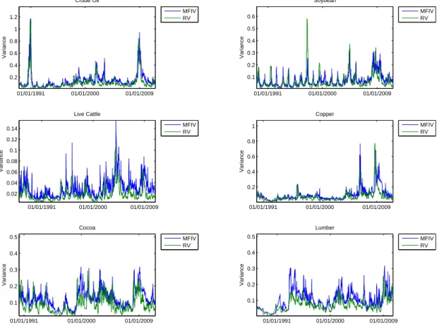
Prior to discussing our empirical results, it is instructive to visualize the time series dynamics of realized variance (RV) and model-free implied variance (MFIV). Figure 1 plots these series for 6 commodities drawn from different sectors. This figure highlights several interesting features. First, RV and MFIV trend together. Second, MFIV is usually higher than RV, suggesting that short variance swaps investments are profitable. However, by visually inspecting these plots, it is difficult to ascertain
9
Ideally, one should report the average open interest and trading volume for the full sample period. Alas, the CRB does not provide such information. Fortunately, the exchanges provide volume data for the very recent years. We use the option trading volume for the period 2010–2011 as an indication of trading activity in commodity markets. SectionE.6 establishes the robustness of our findings to liquidity concerns.
10
The reason for selecting the second and third nearby futures contracts is that, unlike other commodities, energy commodities have a monthly expiration schedule.
whether these profits are significantly different from zero or whether similar results are obtained for other commodities. Third, the scales of the vertical axes indicate that some commodities are more volatile than others, prompting us to explore the connection between variance risk premia and variance levels. We elaborate on each of the above observations in the ensuing paragraphs.
A.
Is Variance Risk Priced in Commodity Markets?
We start our empirical analysis by ascertaining whether variance risk is priced in commodity markets. If variance risk is priced, we expect the average pay-off to variance swaps to be of economically large magnitude and statistically significant.
A.1 Variance Swap Payoffs
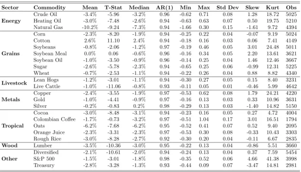
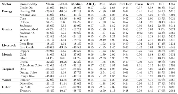
Table 3 presents summary statistics of the estimated commodity variance risk premia. The average 60 day variance risk premia reported in Panel A are mainly negative, suggesting that variance risk is negatively priced in commodity markets. To assess the significance of variance risk premia, we report Newey-West t-statistics in the fourth column of Table 3. The evidence for 60 day variance risk premia (Panel A) suggests that variance swaps generate significant pay-offs in virtually all markets. Unlike individual stocks, we find clear evidence of significantly negative variance risk premia in 17 of the 21 markets.
The volatility of 60 day variance risk premia is generally low, with values usually below 7 %. However, natural gas and coffee variance risk premia exhibit volatilities that are an order of magnitude higher (15 % and 17 %, respectively). The high volatility of silver’s variance risk premium could explain why its market price of variance risk is not statistically different from zero. Examining the higher moments of variance risk premia, we find evidence of positive skewness which contrasts with
the negative skewness often found in returns. The positive skewness indicates
that, though short variance swap positions yield statistically and economically significant profits, these strategies could incur severe losses. Variance risk premia are leptokurtic with kurtosis as high as 24.48 in the soybeans market.
To gain insights into the slope of the short-end of the term-structure of variance risk premia, we repeat the above analysis for 90 day variance risk premia and present the results in Panel B of Table 3. Generally, we observe significantly negative variance swap payoffs in 14 markets, indicating that variance risk is consistently negatively priced across both the bimonthly and quarterly maturities.
In summary, Table 3 unequivocally points to significantly negative variance risk premia in most commodity markets. Moreover, our evidence of significant variance risk premia for most commodities differs from that of individual equities reported in Carr and Wu (2009) and Driessen et al. (2009). This finding underscores the differences between the two asset classes.
A.2 Variance Swap Returns
To better appreciate the profitability of variance swap contracts, we compute the Log Variance Risk Premium (LVRP) defined as the continuously compounded excess return on a fully collateralized variance swap position. More formally, the variance swap return for the period from time t to T is computed as follows: LV RPt,T =
logh RVt,T
M F IVt,T i
.
Table 4 displays the results of the analysis for the LVRP. Again, we report results for 60 and 90 day variance swaps in Panels A and B, respectively. The LVRPs reported in Panel A of Table 4 are mostly negative.11 The standard deviation of
LVRPs is fairly homogeneous across commodities with values typically below 50 %. To better appreciate the risk/reward characteristics of commodity variance swaps, we report absolute values of annualized, Newey-West corrected Sharpe Ratios (SR) in the penultimate column of Table 4. We present absolute values of SR because the negative returns on variance swaps complicate cross-market comparisons of SR. Table 4 demonstrates that 60 day commodity variance swaps yield sizable SR varying
11
It is important to stress that under the null of zero variance risk premium, the average LVRP will be biased towards negative values due to Jensen’s inequality. This observation explains the seemingly conflicting evidence, reported in Carr and Wu (2009), of significantly negative mean LVRP even though the average VRP, itself, is not statistically significant. Driessen et al. (2009) echo a similar concern in their footnote 13.
between 9.4 % and 63.4 %.12 Clearly, these figures are higher than the 10 % that a
long passive investment in commodity futures typically generates (Koijen et al., 2012). The variability in SR within and across sectors is striking. At 2 month horizons, SR fluctuate between 34 % and 47 % in energy markets. This variability carries over to grains and livestocks. For example, a short variance swap position in live cattle earns an annualized SR of 50.2 %, almost three times higher than the 17.4 % of lean hogs.
We further compare the performances of commodity variance swaps of different maturities. We repeat the above analysis for 90 day variance risk premia. Panel B of Table 4 reports SR that are higher than the reward to variability ratio of a passive investment in commodity futures. However, it is worth noticing that these SR are generally lower than those presented in Panel A, indicating a downward sloping term structure of SR.
B.
Time Variation in Variance Risk Premia
In the following paragraphs, we analyze time variations in variance risk premia. First, we study the link between historical variance levels and variance risk premia. Second, we analyze the dynamics of commodity variance risk premia across different market regimes.
B.1 Affine Premia
We begin by investigating whether variance risk premia are linearly related to historical variance. This is important because most option pricing models assume that variance risk premia are affine functions of the variance of the underlying. Previous studies on variance risk premia, e.g. Carr and Wu (2009) and Trolle and
12
In comparison, Carr and Wu (2009) report SR that vary between 0 % and 55 % for individual US equities.
Schwartz (2010), estimate a regression of the form:13
RVt,T −M F IVt,T =α+βM F IVt,T +ǫ. (6)
Although intuitive, this approach can be criticized on two grounds. First, the regression suffers from the issue of endogeneity, which biases the slope estimate. This problem arises because the variance risk premium affects the MFIV, which appears on both sides of the equation. Second, Equation (6) is likely to be an imbalanced regression since the order of integration of the variable on the left is smaller than that of the independent variable.14 To address these issues, we build
on the arguments of Bollerslev et al. (2013) and run the following regression:15
RVt,T −M F IVt,T = ˜α+ ˜βHISTt+ǫ. (7)
where RVt,T is the realized variance between times t and T. M F IVt,T is the
model-free implied variance between times t and T. HISTt is the fractionally differenced
historical variance. As is standard in the literature, we set the order of fractional integration at 0.40.
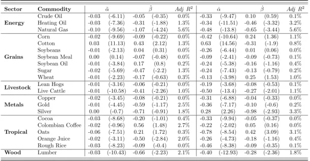
The first five columns of Table 5 report the results from Regression (7). Starting with 60 day variance risk premia, we find that the slope estimates are generally not statistically distinguishable from zero. This result suggests that commodity variance risk premia are unrelated to historical variance. We also assess whether variance swap returns are time varying by estimating the following regression:
log(RVt,T)−log(M F IVt,T) = ˙α+ ˙βlog(HISTt) +ǫ. (8)
where log(RVt,T) is the log realized variance between times t and T. log(M F IVt,T)
is the log model-free implied variance between times t and T. log(HISTt) is the 13
It is straightforward to rearrange the regression models presented in Carr and Wu (2009) and Trolle and Schwartz (2010) to obtain Equation (6).
14
Note that the dependent variable is the difference of two series, making its order of integration smaller than that of the original series.
15
(fractionally) differenced logarithm of historical variance. The last five columns of Panel A report the coefficients, t-statistics and R2 of the above regression. The main findings do not change. We cannot reject the null hypothesis at the 5 % level in most markets.
Panel B of Table 5 presents our findings for variance swaps that mature in 3 months. Our main conclusion is unaltered: the profitability of short variance swaps positions is unrelated to historical variance.
Overall, our results suggest that the market price of commodity variance risk is not an affine function of variance. This result directly contradicts that of Carr and Wu (2009) and Trolle and Schwartz (2010). We attribute the difference in results to our more robust econometric approach that allows us to address the issues of endogeneity and imbalanced regressions.16
B.2 Market Regimes
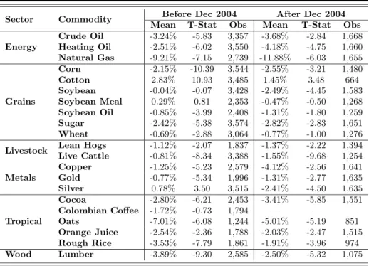
In order to analyze the dynamics of commodity variance risk premia across different market regimes, we partition our sample into 2 distinct periods: the first period
ends in November 2004, the second subsample runs from December 2004 onward.17
These periods are selected because of their economic importance. The first
subsample, which we refer to as “pre-financialization”, corresponds to a period of low investor participation in commodity markets. The second period coincides with the financialization of commodity markets, a period characterized by increased investor flows into commodities. The results are presented in Table 6.
We confirm that variance risk is significantly priced in commodity markets during each of the two periods analyzed. Our results point to consistently negative variance risk premia for most markets. Moreover, for each commodity market, the variance risk premia estimates are of similar order of magnitude in each of the
16
To verify this, we follow the steps outlined in Carr and Wu (2009) and Trolle and Schwartz (2010). Their approach, which suffers from both endogeneity and imbalanced regression concerns, leads us to the conclusion that variance risk premia are affine functions of variance. The details of this analysis are not reported for brevity.
17
In a recent study, Hamilton and Wu (2014) document a structural break in crude oil’s futures risk premia in December 2004. Other studies argue in favour of 2005 as a breakpoint. Considering 2005 as a breakpoint leads to very similar results. These results are not reported for brevity.
two subsamples. Collectively, these results show that variance risk premia are fairly consistent by commodity, and consistently negative overall, in both sample periods.18
C.
Commonalities in Variance Swap Returns
We now investigate commonalities in variance swap returns. We follow a two-step approach. First, we analyze the correlations across commodities. Second, we study comovements across asset classes.
C.1 Evidence from Commodity Markets
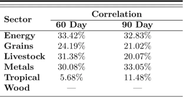
Panel A of Table 7 presents the average correlation within each commodity sector. These figures are computed as follows. For each sector, e.g. energy, we compute pair-wise correlations between the variance swap returns of constituent commodities. We then average all pair-wise correlations to obtain the correlation within a sector. Note that we do not perform this analysis for the wood sector because it contains only one commodity (lumber). The estimated correlations vary between 5.68 % (tropical) and 33.42 % (energy) for 60 day variance swap returns, indicating mild comovements within individual sectors. Similarly, the average correlations of 90 day variance swap returns fluctuate between 11.48 % (tropical) and 33.05 % (metals). In general, these coefficients point to moderate commonalities within commodity sectors.
We now extend our analysis by studying commonalities across (rather than within) commodity sectors. Each trading day, we calculate the return on an equally-weighted portfolio of variance swaps of all commodities involved in a specific sector. By doing so, we obtain time series of variance swap returns for each sector. Next, we compute pair-wise correlations across different sectors. Panels B and C of Table 7
18
These findings have a more profound implication. In particular, they suggest that liquidity effects are unlikely to drive our results. To understand this, remember that the second sample period relates to a period of high trading activity in commodity markets. If liquidity drove our results, one should observe marked differences across both sample periods. Clearly, our results suggest that the results for the two samples are broadly similar, making liquidity-based stories difficult to reconcile with the data. SectionE.6 digs deeper into the issue of liquidity and presents a variety of analyses that further establish the robustness of our findings.
report the correlations of variance swap returns across sectors. We observe moderate correlations across sectors. The reported figures vary from 6.54 % (livestock and metals) to 24.65 %, (grains and tropicals) at the shorter horizon.19
The relatively moderate correlations across commodity variance swap returns suggest that a diversified portfolio of commodity variance swaps might have desirable features. We verify this by computing the, Newey-West corrected, annualized SR of a portfolio of variance swaps. On each day, we take an equally-weighted short position in all available variance swaps of a specific maturity. Since we do not have options data for most commodities in the year 1989, we construct the diversified portfolio from 1990 onward. On average, the diversified portfolio comprises 15 commodity markets. Focusing on the entries reported under “Diversified” in Table 4, we can see that a short equally-weighted portfolio of commodity variance swaps generates returns of 21.1 % and 19 % at the 60 and 90 day horizon, respectively. The diversified portfolio performs well compared to individual commodity variance swaps as its reward to variability ratio is equal to 37.9 % and 23.6 % for the shorter and longer maturities, respectively.
C.2 Evidence from Equity and Bond Markets
We also analyze comovements between commodity variance swap returns and those observed in equity and fixed-income markets. To this end, we use options data on the S&P 500 index and the 30-Year US Treasury bond. Our data comes from OptionMetrics and covers the periods 1996–2011 and 1996–2010 for the equity and fixed-income market, respectively.20 We follow the steps outlined in Section II to
19
We also perform a principal component analysis (PCA). The results, not reported here for brevity, suggest that five factors are necessary to explain variations in variance swap returns across sectors with each factor capturing roughly 20 % of common variations.
20
Our sample period for the S&P 500 and Treasury markets is determined by the availability of data from OptionMetrics. In general, the sample period for the bond and equity markets is shorter than that of most commodities. One should bear this in mind when interpreting our results.
estimate the variance risk premia of these markets.21 We then compute the pair-wise
correlations between the variance swap returns of individual commodity sectors and those of the stock and bond markets. Rows “S&P 500” and “Treasury” of Table 7 summarize our findings. We observe (at most) moderate comovements between bond and equity variance swap returns on the one hand and commodity variance swap returns on the other. For example, the correlation between energy and equity (bond) variance swap returns is 26.50 % (20.18 %) at the bimonthly horizon.
Motivated by the literature on the financialization of commodities, we analyze
how the markets comove at different points in time. To this end, we repeat
our analysis for each of the two regimes discussed in Section B.2. As Table 8
demonstrates, there are important differences between the two time periods. For example, the correlation between energy and equity variance risk premia is low (2.62 %) during the first sub period. However, it soars to 47.50 % in the second
subsample. More generally, we can clearly see that variance swap returns are
strongly correlated with each other during the “financialization” subsample. This stylized fact amounts to direct and model-free evidence that the financialization of commodity markets documented by Tang and Xiong (2012) affects not only the risk premia associated with the first but also the second moment of commodity returns. Taken as a whole, we find some commonalities in variance swap returns across asset classes. Our findings show that commodity variance swap returns are increasingly integrated with those of the bond and equity markets, indicating that the financialization of commodity markets is a general phenomenon that affects not only price risk premia but also variance risk premia.
21
The last two entries of Tables 3 and 4 report summary statistics of bond and equity variance and log variance risk premia, respectively. Briefly, we can see that variance risk is negatively priced in both markets. This is true for both the shorter and longer maturities. More interestingly, a short position in the S&P 500 yields an annual reward to variability ratio of around 37 %. This is important for two reasons. First, it indicates that a portfolio of commodity variance swaps performs as well as a short position in the S&P 500 variance swap. Moreover, the Sharpe Ratio of the short S&P 500 variance swap position is much smaller than the 0.98 documented by Carr and Wu (2009) at the monthly horizon. While this result may be due to a downward sloping term-structure of variance risk premia, it could also highlight the importance of analyzing variance swaps over a long period to draw robust inferences.
D.
Price v.s. Variance Risk Premia
Having documented the existence of time varying variance risk premia, we now turn our attention to the relationship between price and variance risk premia. To do so, we proceed in several steps. First, we examine the relationship between equity and bond risk premia on the one hand and commodity variance risk premia on the other. Second, we focus on the link between the variance swap returns of a commodity and its future returns.
D.1 Equity Risk Premia
It is natural to wonder whether variance swap returns are linked to the systematic factors that drive equity risk premia. After all, the negative sign of the market price of variance risk may be consistent with the Capital Asset Pricing Model (CAPM) and its extensions. Specifically, if an asset’s volatility is negatively related to the market return, as is the case in equities, then one would expect a negative variance risk premium.
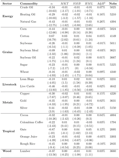
We analyze the relationship between variance swap returns and the 3 factors of Fama and French (1993). We obtain our data from French’s website and estimate the following regression for each commodity:
LV RPt=α+βM KTt+γSM Bt+δHM Lt+ǫt. (9)
where LV RP, M KT, SM B and HM L denote the time series of variance swap
returns, the market, small minus big and high minus low factors, respectively. Tables 9–10 report our main results. We can see highly significant intercepts and, in most cases, statistically insignificant slope estimates, which indicate that commodity variance swap returns are largely orthogonal to the equity risk premium. Furthermore, the three factors typically account for less than 1 % of variations in commodity variance swap returns, leading us to conclude that commodity variance swap returns cannot be satisfactorily explained by the Fama and French (1993) factors.
D.2 Bond Risk Premia
We now investigate how the determinants of bond risk premia relate to variations in commodity variance swap returns. We draw upon the work of Ludvigson and Ng (2009), who implement a dynamic factor analysis decomposition to extract 8 factors from a panel of 132 macroeconomic variables. We also use the Cochrane and Piazzesi (2005) factor, which has been shown to explain bond risk premia. All data are downloaded from Ludvigson’s website.22
Table 11 presents the results of regressions of 60 day variance risk premia on these factors. On average, the regression yields significant intercepts of large
magnitude and very low explanatory power. We find negative Adj R2 in 10 out
of 21 markets. The cross-sectional average Adj R2 is less than 3 %, signaling that commodity variance swap returns are not affected by the drivers of bond risk premia. The coefficient estimates are of very low magnitude, with each factor exhibiting only 3 significant test statistics across all 21 markets. We obtain similar results for variance swaps of 90 day maturity (see Table 12). Clearly, the determinants of bond risk premia cannot explain movements in commodity LVRP satisfactorily.
D.3 Commodity Price Risk Premia
To analyze the relationship between commodity variance risk premia and commodity price risk premia, we regress variance swap returns on futures returns computed as follows RETt,T = 252 T −t T X i=t+1 log Fi,T Fi−1,T (10) 22
Note that the monthly series of macro factors stops in December 2003. We restrict our sample of variance swap returns accordingly.
where Fi,T denotes the futures contract observed at time i and expiring at time
T.23,24 If price and variance risk premia are highly related, we expect to see a high
explanatory power and significant slope estimates.
Table 13 displays statistically significant intercept estimates in all markets. More importantly, the intercepts are remarkably similar to the unconditional LVRP presented in Table 4. Of the 21 time series of commodity variance swap returns, only 6 exhibit a statistically significant relationship with futures returns. This suggests that there is a weak relationship between price and variance risk premia. This result is further corroborated by the low explanatory power (typically lower than 6 %).
Summarizing, we provide model-free evidence of unspanned stochastic variance in commodity markets: stochastic variance is not spanned by a long position in a single futures contract. A direct implication of this result is that term structure models of commodity futures must allow for both spanned and unspanned stochastic variance. In future work, it would be interesting to dig deeper into this class of models. Trolle and Schwartz (2009) provide an interesting starting point.
E.
Robustness Analysis
In this section, we establish the robustness of our findings. To begin with, we demonstrate that our main results hold when we analyze the expected (as opposed to realized) market price of variance risk. Next, we show that our findings are robust to the interpolation technique. We then confirm that the choice of truncation points does not materially affect our main results. Subsequently, we demonstrate that our approach yields implied volatility indices that correlate very well with (the handful of) publicly available volatility indices. We also show that liquidity concerns do not materially change our main findings. Additionally, we analyze the impact of
23
Including the Goldman Sachs Commodity Index (GSCI) in our regression model does not materially affect our results. These are not reported for brevity.
24
An alternative approach consists in identifying and using factors that explain variations in commodity futures returns. Alas, it is not entirely clear which factors (if any) successfully price commodity futures returns (Daskalaki et al., 2014; Szymanowska et al., 2014). Our direct approach, which broadly mirrors that of the literature on unspanned stochastic volatility, allows us to conveniently sidestep this fiercely debated issue by directly using commodity futures risk premia in the regression model.
seasonality on our main results. Lastly, we repeat our analysis using non-overlapping data and confirm that our main results hold.
E.1 Expected Variance Risk Premia
Although consistent with the market definition of variance swap payoffs, it is important to acknowledge that our estimates of variance risk premia implicitly assume that realized variance is equal to the physical expectation of variance. Strictly speaking the variance risk premium is equal to the difference between the physical and risk-neutral expectations of variance. Viewing realized variance as the sum of the physical expectation of variance plus a forecasting error, our evidence of negative variance risk premia could be taken as evidence that the mean forecasting error is negative. Thus, it appears important to also analyze the expected market price of variance risk.
Following Bollerslev et al. (2009), we use historical (rather than realized) variance as the floating leg of our variance swap and repeat our analysis. Before discussing the results of this exercise, it is important to stress that the analysis assumes that investors use historical variance to form their expectation about future
variance, making the results somewhat model dependent.25 In a recent study,
Bekaert and Hoerova (2014) provide a detailed discussion of this issue and warn that findings based on expected (as opposed to realized) variance risk premia must be interpreted cautiously.
Tables 14 and 15 present the results of this analysis. Typically, expected and realized variance swap returns display a correlation coefficient that is lower than 40 %. More important, investors expect significantly negative variance risk premia in most commodity markets. This result holds for both the bimonthly and quarterly maturities, strengthening our main conclusions.
25
It is outside of the scope of this paper to identify the best forecasting model of variance. See Andersen et al. (2009) for a recent survey of the literature on variance forecasting.
E.2 Interpolation Technique
We evaluate the robustness of our results to the interpolation technique. To this end, we follow the procedure outlined in Section II with one difference: we use a cubic spline (rather than linear) interpolation technique to obtain a fine grid of implied volatilities. Tables 16 and 17 demonstrate that our results are robust to the interpolation technique. In particular, Column “Corr” shows that the variance risk premia estimated using the spline interpolation technique and that obtained using the linear interpolation are highly correlated. Typically, this correlation coefficient is greater than 99.9 %. Our main conclusions are unchanged: commodity variance risk premia are significantly negative and of economically large magnitude.
E.3 Truncation Points
We also investigate the sensitivity of our variance swap estimates to the truncation points. We work with tighter truncation points, Kl and Ku, defined as follows:
Kl = Ft,T exp
−8σT
(11)
Ku = Ft,T exp8σT (12)
where Kl and Ku refer to the lower and higher truncation points. Ft,T refers to
the futures contract observed at time t and expiring at T,σ is the average implied
volatility of all OTM options and T denotes the time to maturity of the option
contract.
As Tables 18 and 19 clearly show, our findings are not materially affected by this change. In fact, the numbers reported under “Corr” show that the correlation between the newly estimated variance risk premia and our benchmark estimates is typically greater than 99.9 %. In short, our results are robust to the choice of truncation points.
E.4 The Role of Jumps
We now examine the robustness of our results to the presence of jumps. This is important because jumps could affect the replication of variance swap rates. In a recent study, Rompolis and Tzavalis (2013) show how to gauge the bias induced by jumps. They formally prove that the bias due to jumps (JB) is related to the model-free skewness (MFS) and kurtosis (MFK):
JBt,T = − 2ert(T−t) T −t 1 3!M F St,T + 1 4!M F Kt,T (13) M F St,T = Z +∞ Ft,T 6 log[ K Ft,T]−3 (log[ K Ft,T]) 2 K2 C(t, K, T)dK (14) − Z Ft,T 0 6 log[ K Ft,T] + 3(log[ K Ft,T]) 2 K2 P(t, K, T)dK (15) M F Kt,T = Z +∞ Ft,T 12(log[ K Ft,T]) 2 −4 (log[FKt,T]) 3 K2 C(t, K, T)dK (16) − Z Ft,T 0 12(log[ K Ft,T]) 2+ 4(log[ K Ft,T]) 3 K2 P(t, K, T)dK (17)
whereJBt,T refers to the bias due to jumps. The annualized risk-free rate is denoted
byrt. Ft,T denotes the futures contract observed at timetand expiring atT. M F St,T
and M F Kt,T denote the risk-neutral skewness and kurtosis, respectively. P(t, K, T)
and C(t, K, T) denote the price at time t of European put and call options struck at K and expiring atT.
Following Rompolis and Tzavalis, we add together the MFIV and the JB to obtain a jump robust estimate of the risk-neutral expectation of variance. We then repeat our analysis of variance risk premia and variance swap returns. Tables 20 and 21 demonstrate that accounting for the role of jumps does not change our main findings. We still observe significantly negative variance risk premia in most commodity markets, strengthening the conclusion that short variance swap positions are highly profitable in commodity markets.
E.5 Synthetic v.s. Public Volatility Indices
We compare our synthetic swap rates to publicly available volatility indices. Since our methodology broadly mirrors that of the exchange, we expect the synthetic and publicly available variance swap rates to be highly correlated. Although there are volatility indices for the corn, soybeans and wheat markets, these indices were only recently introduced. Hence, we focus only on the crude oil and gold markets. There are, however, 2 issues that need to be highlighted. First, the crude oil volatility index reported by the exchange is based on a 30 day horizon. In contrast, our synthetic variance swap rates are available for horizons of both 60 and 90 days. To ensure a valid comparison, we create synthetic variance swaps of 30 days for the crude oil market.26 These variance swaps are used solely for comparison purposes and are not
discussed further in the paper. Second, the exchange lists the model-free implied volatility rather than variance. As a result, we square the volatility indices in order to make them comparable to our variance swap rates.
The comparison period extends from May 11, 2007 to September 2, 2011 for crude oil. Similarly, the period of interest starts from September 13, 2010 to August 10, 2011 for gold. Overall, the overlapping periods comprise 1078 and 227 days for the crude oil and gold markets, respectively. We proceed in two steps. First, we compute the correlation between our synthetic variance swap rates and the CME series. As expected, we observe a high correlation between the two series. The correlation coefficients are equal to 97.38 % and 98.04 % for the crude oil and gold markets, respectively. Second, we analyze the mean difference. On average, our synthetic variance swap rate is very close to its CME counterpart. For example, the synthetic swap rate of gold differs from that of the exchange by an average of 11 basis points. In summary, this analysis gives us confidence in our empirical methodology.
26
Note that the construction of monthly variance swaps is not possible for non-energy commodities. This is due to the fact that non-energy commodity options do not have monthly expiration cycles.
E.6 Tradability of Commodity Variance Swaps
Studies on variance risk premia, including those of Carr and Wu (2009) and Driessen et al. (2009), are invariably criticized on the grounds that option contracts may not be actively traded and this may significantly drive the results. We argue that this is unlikely to be true in our case for several reasons. First, the evidence of significantly negative variance risk premia is not specific to a limited number of commodity markets. Rather this finding holds for virtually all commodity markets, making a liquidity-based explanation of our results very challenging. Second, if the lack of liquidity significantly drove our results, one would observe large differences in the magnitude, sign, and statistical significance of the variance risk premia during the“financialization” period, where commodities grew in popularity. However, as Table 6 clearly shows, the sign and magnitude of commodity variance risk premia is stable across both the “pre-financialization” and “financialization” samples, making our results difficult to reconcile with a liquidity-based story.
Another potential concern is that the performance of the diversified portfolio of commodity variance swaps is difficult to achieve in practice because it includes less actively traded commodity markets. To address this concern, we construct an equally-weighted portfolio of commodity variance swaps that includes the 7 most actively traded commodities. To identify these actively traded commodities, we
use the yearly average option trading volume reported in Table 1.27 The seven
markets include corn, crude oil, gold, natural gas, soybeans, sugar and wheat.28 Our
unreported analysis indicates that the newly constructed portfolio yields SR equal to 36.01 % and 17.04 % for the shorter and longer horizons, respectively. Overall, these
27
To a large extent, the decision to look at the option trading volume for the period 2010–2011 is forced upon us, as the CRB data set does not contain information on the trading volume of individual options. As a further robustness check, we obtain the yearly average futures trading volume for the period 1989–2011 from Bloomberg. We then create another portfolio that includes the 7 commodities with the highest average futures (rather than option) trading volume and obtain very similar results. This is hardly surprising because 6 (of the 7) commodity markets with the highest average option volume are also among the 7 markets with the highest average futures trading volume.
28
It is worth pointing out that corn, crude oil, gold, soybeans and wheat now have publicly available volatility indices. This highlights the importance of these markets from a trading perspective.
reward-to-variability ratios are very similar to those reported for the unrestricted portfolio of commodity variance swaps (see Table 4). The upshot of this is that our main findings are robust to liquidity concerns.
One may also wonder about the impact of transaction costs on our variance risk premia estimates. It may be that our synthetic variance swap rate are the sum of the true variance swap rate and transaction costs. It is therefore possible that the variance risk premia estimates presented in Table 3 are biased downwards, i.e. more negative than the true variance risk premia, owing to the influence of transaction costs. To investigate this, we incorporate transaction costs in our analysis. We follow two approaches. First, we assume that transaction costs represent 5 % of the synthetic variance swap rate. This implies that the true variance swap rate corresponds to 95 % of the synthetic variance swap rate. For example, if the synthetic variance swap rate is 10% the true variance swap rate is 9.5 %. Second, we allow for fixed transaction costs in the spirit of Duarte et al. (2007), by assuming that the true model-free implied volatility (not variance) is 1 % less than the synthetic model-free implied volatility. This means that if the synthetic model-free implied volatility is 10 %, then the true implied volatility is 9 %, leading to a true variance swap rate of 0.81 %. It is worth noticing that this approach is generally more stringent than the proportional approach, thus yielding very conservative variance risk premia estimates. Tables 22–23 summarize our main results. Although we observe slightly less negative variance risk premia for most commodity markets, we can see that most variance risk premia remain significantly negative. This is true regardless of whether we assume proportional or fixed transaction costs.29 Collectively, these
analyses indicate that our results are not driven by the effect of transaction costs.
29
We go a step further and assume that the manager of a portfolio of short variance swaps charges performance fees equal to 20 % of the payoff to variance swaps. This implies that the net-of-fees variance risk premia corresponds to 80 % of the figures reported under Tables 22–23. More importantly, the t-statistics of the net-of-performance-fees variance risk premia correspond to approximately 0.9(√0.8) of those shown in Tables 22–23. Clearly, the significance of our main findings is robust to this.
E.7 Seasonality in Commodity Variance Swap Returns
Many commodities exhibit seasonal patterns. Suenaga et al. (2008) document the seasonality of realized variance in the natural gas market. More recently, Back et al. (2013) find evidence of seasonality in implied volatilities. One may wonder how this salient feature of commodity markets affects our analysis of commonalities.
To address this concern, we deseasonalize variance swap returns by regressing individual series on twelve monthly dummies. We then use the deseasonalized series to repeat all our analyses. Focusing on our investigation of commonalities across markets, Table 24 reports similar results to our baseline estimates (see Table 7). Clearly, accounting for calendar variations in commodity variance swap returns does not materially affect our results.
E.8 Non-Overlapping Samples
Although the various statistics displayed in Table 3 are compelling, they are subject to a potential problem: we estimate realized variance on a rolling window basis. It could be argued that because of the substantial amount of overlap in sampling periods, our results may not be particularly informative. To address such concern, we present summary statistics of non-overlapping variance risk premia in Table 25. Overall, the results are quite similar to those reported in Table 3. The reduction in the autocorrelation of variance risk premia is noteworthy. For example, the autocorrelation of gold’s 60 day variance risk premium falls from 0.97 to 0.21. This is not surprising, given that there is no overlap between consecutive variance swap contracts. Although we observe differences for some commodities, e.g. lean hogs, the results are generally quite similar to those reported in Table 3. In short, variance risk is significantly priced in commodity markets.
IV
Conclusion
This paper investigates the market price of variance risk in 21 commodity markets from 1989 to 2011. Using synthetically constructed variance swaps, we present
model-free evidence of variance risk premia in commodity markets. More specifically, we show that variance risk is negatively priced in most commodity markets. A portfolio of short commodity variance swaps significantly outperforms that of long commodity futures, highlighting the potential benefits of investing in variance derivatives. Our results hold for variance swap contracts that mature in either 60 or 90 days and we confirm that variance risk is priced during both the “pre-financialization” and “financialization” sample periods.
We find some evidence of commonalities in variance swap returns both within and across commodity sectors. More important, we document increasing comovements between commodity variance swap returns on the one hand and bond and equity variance swap returns on the other. In short, our findings suggest that the financialization of commodity markets is not restricted to futures markets: it also affects the market for variance swaps.
Finally, we show that commodity variance risk premia are distinct from traditional risk premia. In particular, we establish that the Fama and French (1993) and the Ludvigson and Ng (2009) factors, which successfully capture equity and bond risk premia, cannot explain commodity variance swap returns satisfactorily. Moreover, regressing commodity variance risk premia on price risk premia, we find that the two risk premia are distinct, i.e. variance risk is unspanned by commodity futures.
References
Andersen, T., Bollerslev, T., and Diebold, F. (2009). Parametric and nonparametric
volatility measurement. Handbook of Financial Econometrics: Tools and
Techniques, 1:67.
Back, J., Prokopczuk, M., and Rudolf, M. (2013). Seasonality and the valuation of commodity options. Journal of Banking & Finance, 37(2):273–290.
Bakshi, G. and Kapadia, N. (2003a). Delta-hedged gains and the negative market volatility risk premium. Review of Financial Studies, 16(2):527–566.
Bakshi, G. and Kapadia, N. (2003b). Volatility risk premiums embedded in
individual equity options. Journal of Derivatives, 11(1):45–54.
Barone-Adesi, G. and Whaley, R. (1987). Efficient analytic approximation of
american option values. Journal of Finance, 42(2):301–320.
Bekaert, G. and Hoerova, M. (2014). The VIX, the variance premium and stock market volatility. Forthcoming in Journal of Econometrics.
Black, F. (1976). The pricing of commodity contracts. Journal of Financial
Economics, 3(1):167–179.
Bollerslev, T., Osterrieder, D., Sizova, N., and Tauchen, G. (2013). Risk and return: Long-run relations, fractional cointegration, and return predictability. Journal of Financial Economics, 108:409–424.
Bollerslev, T., Tauchen, G., and Zhou, H. (2009). Expected stock returns and variance risk premia. Review of Financial Studies, 22(11):4463–4492.
Britten-Jones, M. and Neuberger, A. (2000). Option prices, implied price processes, and stochastic volatility. Journal of Finance, 55(2):839–866.
Broadie, M., Chernov, M., and Johannes, M. (2007). Model specification and risk premia: Evidence from futures options. Journal of Finance, 62(3):1453–1490.
Carr, P. and Wu, L. (2009). Variance risk premiums. Review of Financial Studies, 22(3):1311–1341.
Cochrane, J. and Piazzesi, M. (2005). Bond risk premia. American Economic
Review, pages 138–160.
Coval, J. and Shumway, T. (2001). Expected option returns. Journal of Finance, 56(3):983–1009.
Daskalaki, C., Kostakis, A., and Skiadopoulos, G. (2014). Are there common factors in commodity futures returns? Journal of Banking and Finance, 40:346–363. Demeterfi, K., Derman, E., Kamal, M., and Zou, J. (1999). A guide to volatility
and variance swaps. Journal of Derivatives, 6(4):9–32.
Driessen, J., Maenhout, P., and Vilkov, G. (2009). The price of correlation risk: Evidence from equity options. Journal of Finance, 64(3):1377–1406.
Duarte, J., Longstaff, F. A., and Yu, F. (2007). Risk and return in fixed-income
arbitrage: Nickels in front of a steamroller? Review of Financial Studies,
20(3):769–811.
Fama, E. F. and French, K. R. (1993). Common risk factors in the returns on stocks and bonds. Journal of Financial Economics, 33(1):3–56.
Gorton, G. B., Hayashi, F., and Rouwenhorst, K. G. (2013). The fundamentals of commodity futures returns. Review of Finance, 17(1):35–105.
Hamilton, J. D. and Wu, J. C. (2014). Risk premia in crude oil futures prices. Journal of International Money and Finance, 42:9–37.
Jiang, G. and Tian, Y. (2005). The model-free implied volatility and its information content. Review of Financial Studies, 18(4):1305–1342.
Koijen, R., Moskowitz, T., Pedersen, L., and Vrugt, E. (2012). Carry. Working
Ludvigson, S. and Ng, S. (2009). Macro factors in bond risk premia. Review of Financial Studies, 22(12):5027–5067.
Mueller, P., Vedolin, A., and Yen, Y. (2013). Bond variance risk premia. Working Paper.
Pan, J. (2002). The jump-risk premia implicit in options: Evidence from an
integrated time-series study. Journal of Financial Economics, 63(1):3–50.
Rompolis, L. S. and Tzavalis, E. (2013). Retrieving risk neutral moments and expected quadratic variation from option prices. Working Paper.
Singleton, K. J. (2014). Investor flows and the 2008 boom/bust in oil prices.
Management Science, 60(2):300–318.
Suenaga, H., Smith, A., and Williams, J. (2008). Volatility dynamics of NYMEX natural gas futures prices. Journal of Futures Markets, 28(5):438–463.
Szymanowska, M., De Roon, F., Nijman, T., and Van den Goorbergh, R. (2014). An anatomy of commodity futures risk premia. Journal of Finance, 69(1):453–482. Tang, K. and Xiong, W. (2012). Index investment and the financialization of
commodities. Financial Analysts Journal, 68(5):54–74.
Taylor, S., Yadav, P., and Zhang, Y. (2010). The information content of implied volatilities and model-free volatility expectations: Evidence from options written on individual stocks. Journal of Banking & Finance, 34(4):871–881.
Trolle, A. and Schwartz, E. (2009). Unspanned stochastic volatility and the pricing of commodity derivatives. Review of Financial Studies, 22(11):4423–4461.
Trolle, A. and Schwartz, E. (2010). Variance risk premia in energy commodities. Journal of Derivatives, 17(3):15–32.
Wang, Z., Fausti, S., and Qasmi, B. (2011). Variance risk premiums and predictive power of alternative forward variances in the corn market. Journal of Futures Markets, 32(6):587–608.
01/01/1991 01/01/2000 01/01/2009 0.2 0.4 0.6 0.8 1 1.2 Crude Oil Variance 01/01/1991 01/01/2000 01/01/2009 0.1 0.2 0.3 0.4 0.5 0.6 Soybean Variance 01/01/1991 01/01/2000 01/01/2009 0.02 0.04 0.06 0.08 0.1 0.12 0.14 Live Cattle Variance 01/01/1991 01/01/2000 01/01/2009 0.2 0.4 0.6 0.8 1 Copper Variance 01/01/1991 01/01/2000 01/01/2009 0.1 0.2 0.3 0.4 0.5 Cocoa Variance 01/01/1991 01/01/2000 01/01/2009 0.1 0.2 0.3 0.4 0.5 Lumber Variance MFIV RV MFIV RV MFIV RV MFIV RV MFIV RV MFIV RV
Figure 1: Time Series of Realized Variance and Model-Free Implied
Variance
This figure displays time series of realized and model-free implied variances for crude oil, wheat, live cattle, copper, cocoa and lumber over a 60 day horizon. The blue and green lines represent model-free implied and realized variances, respectively. The difference between realized and implied variances is the variance risk premium.
Table 1: Overview of Commodities
This table lists all commodities considered. The first two columns report the sector and name of specific commodities. The third column displays the exchange where the futures and options contracts of the commodity are traded. The fourth and fifth columns report the available maturity months and minimum tick sizes of the options contracts as reported by the relevant exchange. The sixth column displays the average yearly option volume (based on the years 2010 and 2011). We extract the volume data from the monthly volume report published on the exchange’s websites.
Sector Commodity Exchange Maturity Months Tick Size Volume Energy
Crude Oil NYMEX January-December 0.01 35,901,515
Heating Oil CME January-December 0.0001 891,918
Natural Gas NYMEX January-December 0.001 25,995,473
Grains
Corn CBOT January, March, May, July, September, November, December 0.25 28,650,380
Cotton ICE March, May, July, October, December 0.01 2,853,173
Soybeans CBOT January, March, May, July, August, September, November 0.25 11,641,356 Soybean Meal CBOT January, March, May, July, August, September, October, December 0.1 984,277 Soybean Oil CBOT January, March, May, July, August, September, October, December 0.01 2,102,072
Sugar ICE March, May, July, October, December 0.01 7,713,957
Wheat CBOT March, May, July, September, December 0.25 4,588,187
Livestock Lean Hogs CME Febuary, April, June, July, August, October, December 0.025 861,942
Live Cattle CME Febuary, April, June, August, October, December 0.025 2,551,210
Metals
Copper COMEX Febuary, April, June, August, October, December 0.0005 12,203
Gold COMEX March, May, July, September, December 0.1 8,905,621
Silver COMEX March, May, July, September, December 0.5 1,882,170
Tropical
Cocoa ICE March, May, July, September, December 1 487,270
Colombian Coffee ICE March, May, July, September, December 0.05 2,464,992
Oats CBOT March, May, July, September, December 0.25 19,020
Orange Juice ICE January, March, May, July, September, November 0.05 195,483 Rough Rice CBOT January, March, May, July, September, November 0.05 37,770
Wood Lumber CME January, March, May, July, September, November 0.1 8,033