Global Sourcing

H

H

I

I

E

E

R

R

Harvard Institute of Economic Research

Discussion Paper Number 2005

Global Sourcing

by

Pol Antras

and

Elhanan Helpman

May 2003

Harvard University

Cambridge, Massachusetts

Global Sourcing

Pol Antràs and Elhanan Helpman

May 1, 2003

Abstract

We present a North—South model of international trade in which diff erenti-ated products are developed in the North. Sectors are populerenti-ated by final-good producers who differ in productivity levels. Based on productivity and sectoral characteristics, firms decide whether to integrate into the production of inter-mediate inputs or outsource them. In either case they have to decide from which country to source the inputs. Final-good producers and their suppliers must make relationship-specific investments, both in an integrated firm and in an arm’s-length relationship. We describe an equilibrium in which firms with different productivity levels choose different ownership structures and supplier locations, i.e., they choose different organizational forms. We then study the effects of within-sectoral heterogeneity and variations in industry characteristics on the relative prevalence of these organizational forms. The analysis sheds light on the structure of foreign trade within and across industries.

Keywords Trade in intermediate inputs, Imperfect contracting, Property

rights, Multinationalfirms.

JEL Classification Numbers D23, F12, F14, F23, L11, L22

∗_{MIT and NBER, and Harvard University, Tel Aviv University, and CIAR, respectively. Antràs}

1

Introduction

Afirm that chooses to keep the production of an intermediate input within its bound-aries can produce it at home or in a foreign country. When it keeps it at home, it engages in standard vertical integration. And when it makes it abroad, it engages in foreign direct investment (FDI) and intra-firm trade. Alternatively, afirm may choose to outsource an input in the home country or in a foreign country. When it buys the input at home, it engages in domestic outsourcing. And when it buys it abroad, it engages in arm’s-length trade. Intel Corporation provides an example of the FDI strategy; it assembles most of its microchips in wholly-owned subsidiaries in China, Costa Rica, Malaysia, and the Philippines. On the other hand, Nike provides an ex-ample of the arm’s-length import strategy; it subcontracts most of its manufacturing to independent producers in Thailand, Indonesia, Cambodia, and Vietnam.

Growth of international specialization has been a dominant feature of the inter-national economy. Amongst the many examples that illustrate this trend, two are particularly telling. Citing Tempest (1996), Feenstra (1998) illustrates Mattel’s global sourcing strategy in the production of its star product, the Barbie doll. “Of the $2 export value for the dolls when they leave Hong Kong for the United States,” he writes, “about 35 cents covers Chinese labor, 65 cents covers the cost of materials,” – which are imported from Taiwan, Japan, and the United States – “and the remainder covers transportation and overheads, including profits earned in Hong Kong” (pp.35-36). The World Trade Organization provides another example in its 1998 annual report. In the production of an “American” car, 30 percent of the car’s value originates in Korea, 17.5 percent in Japan, 7.5 percent in Germany, 4 percent in Taiwan and Singapore, 2.5 percent in the U.K., and 1.5 percent in Ireland and Barbados. That is, “...only 37 percent of the production value... is generated in the United States” (p.36).

Importantly, the increasing international disintegration of production is large enough to be noticed in aggregate statistics. Feenstra and Hanson (1996) use U.S. input—output tables to infer U.S. imports of intermediate inputs. They find that the share of im-ported intermediates increased from 5.3% of total U.S. intermediate purchases in 1972 to 11.6% in 1990. Campa and Goldberg (1997) find similar evidence for Canada and the U.K. (but not for Japan). Hummels, Ishii and Yi (2001), who use a narrower concept of international specialization, i.e., the fraction of imported inputs embodied in the production of goods destined for export, find that in 9 OECD countries and 4

emerging market economies this fraction increased – by almost 30% on average – between 1970 and 1990 (again, not in Japan).1

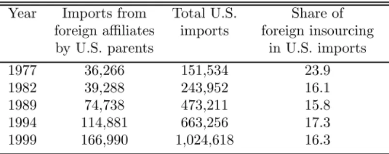
But how important is intra-firm relative to arm’s-length trade in intermediate in-puts? Afirm-level data analysis is needed to answer this question, and no such analysis is available at this point in time. And despite the fact that the business press has stressed the spectacular growth of foreign outsourcing, Hanson, Mataloni and Slaugh-ter (2002) document an equally impressive growth of trade within multinationalfirms. Nevertheless, the fact that imports from foreign affiliates of U.S.-basedfirms has fallen from 23.9% of total U.S. imports in 1977 to 16.3% in 1999, suggests that foreign out-sourcing might have outpaced foreign intra-firm sourcing by U.S.firms.2

Other studies have documented a rise in the prevalence ofdomestic outsourcing by U.S. firms. The Economist (1991), Bamford (1994) and Abraham and Taylor (1996), all report rising subcontracting in particular industries or activities. A systematic analysis of this trend is not available. Nevertheless, Figure 1 provides indirect evidence of a decline in vertical integration. The average number of four-digit SIC segments in which a U.S. publicly-traded manufacturing company operates, declined from 2.72 in

1_{In related work, Yeats (2001) constructs a direct measure of trade in components, taking advantage}

of a recent revision of the Standard International Trade Classification (SITC) system. His data for machinery and transport equipment suggest that, between 1978 and 1995, international trade in components has grown at a faster rate than international trade infinal-stage products.

2

Table 1. Foreign insourcing

Year Imports from Total U.S. Share of foreign affiliates imports foreign insourcing by U.S. parents in U.S. imports 1977 36,266 151,534 23.9 1982 39,288 243,952 16.1 1989 74,738 473,211 15.8 1994 114,881 663,256 17.3 1999 166,990 1,024,618 16.3

Sources: BEA Direct Investment data set and U.S. Census

Table 1 reports data for thefive years in which the BEA conducted comprehensive surveys on the universe of U.S.firms engaging in foreign direct investment. As is evident from the table, the large drop in the share of insourcing occurred sometime between the late 1970s and the early 1980s, and it remained relatively constant during the last 20 years. This share is only a rough measure of the relative importance of foreign insourcing, however, because both the numerator and the denominator include trade infinished goods, and the denominator may also incorporate insourcing by U.S. affiliates of foreign-based multinationals.

Average SIC Segments per Firm year 1979 1982 1985 1988 1991 1994 1997 1.8 2 2.2 2.4 2.6 2.8

Figure 1: The average number of four-digit SIC segments in which firms operate. 1979 to 1.81 in 1997.3 _{The figure suggests that U.S. manufacturing firms have become}

increasingly specialized, which indicates a trend towards less vertical integration. To address issues that arise from the choice of outsourcing versus integration and home versus foreign production, we need a theoretical framework in which companies make endogenous organizational choices. We propose such a framework in this paper by integrating two recent strands of the literature.

Melitz (2002) and Helpman, Melitz and Yeaple (2003) have studied the effects of within sectoral heterogeneity on the decisions of firms to serve foreign markets. By allowing productivity to differ acrossfirms, they show that low-productivityfirms serve the domestic market but not foreign markets, while high-productivityfirms also serve foreign markets. Allowing for horizontal foreign direct investment, Helpman, Melitz and Yeaple also showed that, amongst thefirms that serve foreign markets, the more productive ones engage in foreign direct investment while the less productive firms

3_{The data for thisfigure are taken from Fan and Lang (2000), who constructed it from the}

Com-pustat data set. One might worry that the trend in Figure 1 is driven by a composition effect, i.e., by a relative increase in the number offirms in relatively specialized manufacturing sectors. To examine this possibility, we regressed the four-digit SIC segments per firm on a time trend and firm fixed effects. The coefficient on the time trend was negative, with a T-statistic of₋66.93. We interpret this to imply thatfirms specialized more over time.

export. Importantly, affiliate sales relative to exports are larger in sectors with more productivity dispersion. Their approach emphasized variations across firms within industries, without addressing the organizational choices offirms that need to acquire intermediate inputs.

Grossman and Helpman (2002a) addressed the choice between outsourcing and in-tegration in a one-input general equilibrium framework, assuming that all firms of a given type are equally productive. Theirfirms face the friction of incomplete contracts in arm’s-length relationships, which they weigh against the less-efficient production of inputs in integrated companies. As a result, some sectors have only vertically in-tegrated firms while others have only disintegrated firms. Grossman and Helpman identify sectoral characteristics that lead to one or the other equilibrium structure. This approach has been extended by Antràs (2002a) to a trading environment, by in-troducing two important new features. First, the friction of incomplete contracts also exists within integratedfirms, and – as in Grossman and Hart (1986) – integration provides well defined property rights. However, these property rights may or may not give integration an advantage over outsourcing. Second, there are two inputs, one con-trolled by thefinal-good producer, the other by another supplier, inside or outside the

firm. The relative intensity of these inputs turns out to be an important determinant of the choice between integration and outsourcing.

By embodying this structure in a Helpman and Krugman (1985) style two-sector general equilibrium model of trading countries, Antràs shows that the sector that is relatively intensive in the input controlled by thefinal-good producers integrates, while the sector that is relatively intensive in the other input outsources. As a result, in the former sector there is intra-firm trade in inputs, while in the latter sector there is arm’s-length trade.

Building on this literature, we develop a theoretical model that combines the within-sectoral heterogeneity of Melitz (2002) with the structure of firms in Antràs (2002a). Thefinal-good producer controls the supply of headquarter services while an operator of the production facility of intermediate inputs controls their production. This allows us to explore the joint variations within and across sectors, i.e., productivity within sectors and technological and organizational features across sectors, in shaping organizational forms, trade and foreign direct investment. In particular, we show that in a world of two countries, North and South, in whichfinal-good producers are based in the North,

final-good producers who operate in the same sector but differ by productivity sort into integrated companies that produce inputs in the North (do not engage in foreign trade), integrated companies that produce inputs in the South (engage in FDI and intra-firm trade), disintegrated companies that outsource in the North (do not engage in foreign trade), and disintegrated companies that outsource in the South (import inputs at arm’s length).

We show that in low-headquarter-intensive sectors firms do not integrate; low-productivity firms outsource in the North while high-productivity firms outsource in the South. In sectors with high headquarter intensity all four organizational forms emerge in equilibrium. Importantly, high-productivity firms import inputs while low-productivity firms acquire them in the North. However, amongst the firms that ac-quire inputs in the same country, the low-productivityfirms outsource while the high-productivityfirms integrate. This implies that the least-productive firms outsource in the North while the most productive firms integrate in the South via foreign direct investment.

We use the model to study the relative prevalence of different organizational forms. We show how prevalence depends on the wage gap between the North and the South, the trading costs of intermediate inputs, the degree of productivity dispersion within a sector, the distribution of bargaining power, the size of the ownership advantage (which may be different in the two countries), and the intensity of headquarter services. Our model predicts that relatively morefinal-good producers rely on imported intermediates in sectors with higher productivity dispersion or lower headquarter intensity. And in sectors with integration and outsourcing, which are the sectors with high headquarter intensity, industries with higher productivity dispersion have relatively morefinal-good producers who integrate. This is true for a comparison of integration versus outsourcing in each of the countries. As a result, such sectors have more intra-firm trade relative to arm’s-length trade. These results illustrate the types of issues that can be addressed with our model.

Our model is developed in the next section. In section 3 we characterize an indus-try’s equilibrium. Then, in section 4, we describe the equilibrium sorting of firms into different organizational forms, and we study in section 5 the prevalence of each mode of organization. This is also the section that examines the effects of variations within and across sectors on the relative prevalence of organizational forms. Section 6 offers

a short summary with concluding comments.

2

The Model

Consider a world with two countries, the North and the South, and a unique factor of production, labor. The world is populated by a unit measure of consumers with identical preferences represented by:

U =x0+ 1 µ J X j=1 X_jµ, 0< µ <1,

wherex0 is consumption of a homogeneous good,Xj is an index of aggregate consump-tion in sector j, and µ is a parameter. Aggregate consumption in sector j is a CES function Xj = ·Z xj(i)αdi ¸1/α , 0< α <1,

of the consumption of different varietiesxj(i), where the range ofiwill be endogenously determined. The elasticity of substitution between any two varieties in a given sector is 1/(1 ₋ α). We assume that α > µ, so that varieties within a sector are more substitutable for each other than they are substitutable for x0 or for varieties from a

different sector. This leads to the inverse demand function for each variety i in sector

j:

pj(i) =Xjµ−αxj(i)α−1. (1) In every country the differentiated product sectors are assumed to be small relative to the size of the local labor market. As a result, producers in these sectors face a perfectly elastic supply of labor.4 _{We denote byw}N _{the wage rate in the North and by}

wS the wage rate in the South. These wage rates arefixed and wN > wS.5

The demand parameters µ and α are the same in every industry, which helps to focus attention on cross-sectoral differences in technology and cross-country differences in organizational costs. Our aim is to explore how differences in technology interact

4_{A simple way to ensure this property is to assume that there is a continuum of sectorsj rather}

than afinite number.

5_{The assumption offixed wage rates and a higher wage rate in the North can be justified in general}

equilibrium by assuming thatw is the productivity of labor in producing x0 in country , =N, S, and that labor supply is large enough in every country so that both countries producex0.

with organizational choices in shaping industrial structure, tradeflows and FDI. Only the North has the know-how to produce final-good varieties in the non-homogeneous sectors. To start producing a variety in sector j a firm needs to bear a fixed cost of entry consisting of fE units of Northern labor. Upon paying this fixed cost, the unique producer of variety i in sector j draws a productivity level θ from a known distribution G(θ).6 _{After observing this productivity level, the final-good}

producer decides whether to exit the market or start producing; in the latter case an additionalfixed cost of organizing production needs to be incurred. As discussed below, this additional fixed cost is a function of the structure of ownership and the location of production.

Production of any final-good variety requires a combination of two variety-specific and freely tradable intermediate inputs, hj(i) and mj(i), which we associate with headquarter services and manufactured components, respectively. Output of every variety is a sector-specific Cobb-Douglas function of the inputs,

xj(i) =θ µ hj(i) ηj ¶ηjµ_m j(i) 1₋ηj ¶1−ηj , 0< ηj <1. (2) Notice that, up to the productivity parameter θ, the technology is identical for all varieties in a given sector, but sectors differ in the relative intensity of headquarter services, as represented by η_j. The larger is η_j the more intensive is the sector in headquarter services.

The unit cost function for producing intermediate inputs is identical in all sectors but varies by country. Production of one unit of headquarter services hj(i) in the North requires one unit of Northern labor, while the South is much less efficient at producing headquarter services. We assume that the productivity advantage of the North is so large that headquarter services are only produced in the North. On the other hand, production of one unit of mj(i) requires one unit of labor in the North and in the South.

There are two types of producers: final-good producers and operators of manufac-turing plants for components. Onlyfinal-good producers have the know-how to produce headquarter services. On the other hand, everyfinal-good producer needs to contract with a manufacturing-plant operator for the provision of components. We allow

inter-6_{We can accommodate sectoral differences in thefixed costf}

Eand the distributionG(θ), but chose them to be identical for simplicity.

national fragmentation of the production process, so that the final-good producer can choose to transact with a manufacturing plant in the North or in the South.

It follows from our assumptions thatfinal-good producers locate in the North. Upon paying thefixed cost of entrywN_f

E and observing the productivity levelθ, the unique

final-good producer of variety i in sectorj decides whether to match with an operator of a manufacturing plant in the North or with one in the South. Simultaneously, the

final-good producer chooses whether to vertically-integrate the manufacturing plant or engage instead in an arm’s-length transaction.

We specify a very simple matching technology. After paying thefixed cost of search in a given market, afinal-good producerfinds a match with probability one. We assume that final-good producers in the North need to incur a higher fixed cost to search in the unfamiliar South than in the familiar North. We also assume that the status quo

is for thefirms to remain non integrated. In addition to the search costs, a final good producer incurs management and negotiation costs that depend on the organizational form. All these costs, the sum of which we termfixed organizational costs, are in terms of Northern labor. We denote them by wNf_k, where k is an index of the ownership structure and is an index of the country in which the manufacturing of components takes place.

The ownership structure takes one of two forms: vertical integrationV or outsourc-ingO. The location of the manufacturing of components is in one of two sites: in the NorthN or in the South S. Therefore k _∈{V, O_} and _∈{N, S_}. Anorganizational form consists of an ownership structure and a location for the production of compo-nents. Because the status quo is for the final-good producer to be non-integrated, we assume that the fixed organizational costs are higher for a vertically integrated firm, no matter in which country it owns the manufacturing plant for components. Namely,

f_V > f_O for =N, S.7 _{Note that when a final-good producer owns a manufacturing}

plant of components in the North this represents a standard situation of vertical inte-gration. On the other hand, when afinal-good producer owns the manufacturing plant of components in the South, this represents vertical foreign direct investment (FDI).

We finally assume that the fixed organizational costs are higher in the South,

be-7_{One can imagine situations in which this may not be the case. Nevertheless, we believe that this}

assumption is appropriate in many instances, and we therefore maintain it in the main analysis. It is not difficult, however, to see how various results change when outsourcing requires higherfixed costs. We shall point out how some of the results differ in this case.

cause thefixed costs of search, monitoring, and communication are higher in the foreign country. Combined with the assumption that integration entails higher costs of orga-nization than outsourcing, the fixed organizational costs are ranked as follows:

f_VS > f_OS > f_VN > f_ON. (3) The location of the manufacturing of components and the mode of ownership are chosen ex-ante by thefinal-good producer to maximize the joint value of the relation-ship, as measured by the sum of the operating profits of the final-good producer and the manufacturing plant net of all fixed costs of production. This can be justified by assuming that the final-good producer sets a fee for participation in the relationship that has to be paid by the operator of the manufacturing plant. This fee can be pos-itive or negative, i.e., the operator can make a payment to the final good producer or vice versa. The purpose of the fee is to secure the participation of the operator in the relationship at minimum cost to the final-good producer. When the supply of operators of manufacturing plants is infinitely elastic, the operator’s profits from the relationship net of the participation fee are equal in equilibrium to his outside option.8 For simplicity, we set the operators’ outside option equal to zero. It is, however, easy to extend the analysis to cases in which these outside options are positive and different in the North and in the South.

The setting is one of incomplete contracts. Final-good producers and manufacturing-plant operators cannot sign ex-ante enforceable contracts specifying the purchase of specialized intermediate inputs for a certain price. In addition, the parties cannot write enforceable contracts contingent on the amount of labor hired or on the volume of sales revenues obtained when the final good is sold. One can use arguments of the type developed by Hart and Moore (1999) and Segal (1999) to justify this specification. Namely, that the parties cannot commit not to renegotiate an initial contract and that the precise nature of the required input is revealed only ex-post, and it is not verifiable by a third party. To simplify the analysis, we just impose these constraints on the contracting environment.

Because no enforceable contract can be signed ex-ante, final-good producers and manufacturing-plant operators bargain over the surplus from the relationship after the inputs have been produced. We model this ex-post bargaining as a Generalized Nash

Bargaining game in which thefinal-good producer obtains a fraction β _∈ (0,1) of the ex-post gains from the relationship.9

Following the property-rights approach to the theory of the firm, we assume that ex-post bargaining takes place both under outsourcing and under integration. The distribution of surplus is sensitive, however, to the mode of organization. More specif-ically, the outside option for a final-good producer is assumed to be different when it owns the manufacturing plant than when it does not. In the latter case, a failure to reach an agreement on the distribution of the surplus leaves both parties with no income, because the inputs are tailored specifically to the other party in the transac-tion. However, by vertically integrating the production of components, thefinal-good producer is effectively buying the right to fire the operator of the manufacturing plant and seize the inputs mj(i). If there were no costs associated with firing the operator of the manufacturing plant, the final-good producer would always have an incentive to seize the inputs mj(i) ex-post, and the manufacturing-plant operator would have an incentive to choose mj(i) = 0 ex-ante (which of course would imply xj(i) = 0). In this case integration would never be chosen. We therefore assume that firing the manufacturing-plant operator results in a loss of a fraction 1₋δ of final-good pro-duction.10 _{We also assume thatδ}N _{> δ}S_{. This captures the notion that a contractual} breach is likely to be more costly for thefinal-good producer when the manufacturing plant is located in the South.

3

Equilibrium

Consider the payoffs in the bargaining game for a pair offirms producing in sector j. Since from now on we discuss a particular sector, we drop for simplicity the index j

from all the variables. If the parties agree in the bargaining, the potential revenue from the sale of thefinal goods isR(i) = p(i)x(i), which, using (1) and (2), can be written as R(i) =Xµ−αθα µ h(i) η ¶αηµ m(i) 1₋η ¶α(1−η) . (4)

9_{This specification is similar to Grossman and Helpman (2002a) and Antràs (2002a,b).} 10_{The fact that the fraction offinal-good production lost is independent ofη}

j greatly simplifies the analysis, but it is not necessary for the qualitative results discussed below.

If they fail to agree, however, the outside option for the manufacturing-plant operator is always 0 while that for thefinal-good producer varies with the ownership structure and the location of components manufacturing.

When the final-good producer outsources components, its outside option is also

0 regardless of the location of the manufacturing plant. In this event the final-good producer getsβR(i)while the manufacturing-plant operator gets (1₋β)R(i).

The final-good producer has more leverage under vertical integration. When the parties fail to reach an agreement, the final-good producer can sell an amount δ x(i)

of output when its manufacturing plant is in country , which yields the revenue

¡

δ ¢αR(i). The ex-post gains from trade are in this case h1₋¡δ ¢αiR(i). In the bargaining, the final-good producer receives its default option plus a fraction β of the quasi-rents, i.e. ¡δ ¢αR(i)+βh1₋¡δ ¢αiR(i), while the operator of the manufacturing plant obtains (1₋β)h1₋¡δ ¢αiR(i).

Notice that the payoffs in the bargaining game are proportional to the revenue. Denoting byβ_kR(i)the payoffof thefinal-good producer under ownership structure k

and the location of components manufacturing in country , the assumptionδN > δS

implies that

βN_V =¡δN¢α+β£1₋¡δN¢α¤> βS_V =¡δS¢α+β£1₋¡δS¢α¤> βN_O =βS_O =β. (5) That is,final-good producers are able to appropriate higher fractions of revenue under integration than under outsourcing, with this fraction being higher when integration takes place in the North.

Since the delivery of the inputs h(i)andm(i) is not contractible ex-ante, the par-ties choose their quantipar-ties noncooperatively; every supplier maximizes its own pay-off. In particular, thefinal-good producer provides an amount of headquarter services that maximizesβ_kR(i)₋wN_{h(i) while the manufacturing-plant operator provides an} amount of components that maximizes ¡1₋βk

¢

R(i)₋w m(i). Combining thefi rst-order conditions of these two programs, using (4), the total value of the relationship, as measured by operating profits, can be expressed as:

where ψ_k(η) = 1−α £ βkη+ ¡ 1₋βk ¢ (1₋η)¤ · 1 α ³ wN β_k ´η³ w 1−β_k ´1−η¸α/(1−α) . (7) Note that among the arguments of the profit function π_k(θ, X, η), thefirst one isfi rm-specific while the others are industry-specific. Moreover, while η is a parameter, the consumption indexX is endogenous to the industry but exogenous to the producer of a specific variety of the final good.

Upon observing its productivity levelθ, afinal-good producer either pays thefixed organizational cost wN_f

k and chooses the ownership structure and the location of manufacturing that maximizes (6), or exits the industry and forfeits the fixed cost of entrywN_{fE. It is clear from (6) that the latter occurs whenever θ is below a threshold}

θ, denoted by θ_∈(0,_∞), at which the operating profits

π(θ, X, η) = max

k∈{V,O},∈{N,S}πk(θ, X, η) (8)

equal zero. Namely, θ is implicitly defined by

π(θ, X, η) = 0. (9) This threshold productivity level depends on the sector’s aggregate consumption index

X, i.e.,θ(X).

In solving the problem on the right-hand-side of (8), a final-good producer eff ec-tively chooses the triplet ¡β_k, w , f_k¢ that maximizes (6). It is straightforward to see that π_k(θ, X, η)is decreasing in both w andf_k. For this reason final-good producers prefer to organize production so as to minimize both variable and fixed costs. On account of variable costs, Southern manufacturing is preferred to Northern manufac-turing regardless of the ownership structure (because wN _{> w}S_{). On account of fixed} costs, however, the ranking of profit levels is the reverse of the ranking of fixed cost levels in (3).

Next note that if thefinal-good producer could freely choose its fraction of revenue

β_k, it would chooseβ∗ _∈[0,1]that maximizes ψ_k(η). This fraction is

β∗(η) = η(αη+ 1−α)− p

η(1₋η) (1₋αη) (αη+ 1₋α)

0 1 1 ) ( *_η β η N V β S V β β L η η_H

Figure 2: The Profit-Maximizing Distribution of Revenue

Although a higherβ_k gives thefinal-good producer a larger fraction of the revenue, it also induces the supplier of components to produce fewer components. As a result, the

final-good producer trades the choice of a larger fraction of the revenue for a smaller revenue level.

The functionβ∗(η)is depicted by the solid curve in Figure 2. It rises inη;β∗(0) = 0

andβ∗(1) = 1.11 _{To understand these properties, notice that in the ex-post bargaining}

neither thefinal-good producer nor the manufacturing-plant operator appropriate the full marginal return to their investments in the supply of headquarter services and components, respectively. This leads them to underinvest in the provision of these inputs. Each party’s severity of underinvestment is inversely related to the fraction of the surplus that it appropriates. Ex-ante efficiency then requires giving a larger share of the revenue to the party undertaking the relatively more important investment. As a result, the higher the intensity of headquarter services (the larger isη), the higher is the profit-maximizing fraction of the surplus accruing to the final-good producer (the higher isβ∗).

Following Grossman and Hart (1986), we do not allow a free ex-ante choice of the division rule of the surplus. The choice of ownership structure and the location of the manufacturing of components are the only instruments for affecting the division rule, in the sense that the final-good producer is constrained to choose a β_k in the set ©βNV , β N O, β S V, β S O ª

. When η is close to 1, higher values of βk yield higher profits. Given the ordering in (5), this implies that thefinal-good producer would have chosen domestic integration if there were no other differences in the costs and benefits of the competing organizational forms. Conversely, when η is close to 0, lower values of βk yield higher profits, and the final-good producer would have chosen outsourcing in the absence of other differences in the costs and benefits of the organizational forms.

Naturally, there are other differences in the costs and benefits of various organi-zational forms. As a result, the profit-maximizing choice of an ownership structure and the location of the manufacturing of components depends on afirm’s productivity level. When θ is small, changes in β_k and w have small effects on profits, because changes in ψ_k(η) have small effects on profits (see (6) and (7)). Under the circum-stances differences in fixed costs dominate the choice of an organizational form, which gives domestic outsourcing a particular advantage. On the other hand, whenθ is large,

fixed costs are less important, and the combinations of β_k and w that raiseψ_k(η) as much as possible are particularly advantageous. We shall see in the next section how these tradoffs play out.

Free entry ensures that, in equilibrium, the expected operating profits of a potential entrant equal thefixed cost of entry. From the discussion above, afirm in sectorj that draws a productivity level below θ(X) chooses to exit, because its operating profits are negative. On the other hand, firms withθ _≥θ(X) stay in the industry, and they choose organizational forms that maximize their profits. Under the circumstances the free-entry condition can be expressed as

Z ∞ θ(X)

π(θ, X, η)dG(θ) =wNfE. (11) This condition provides an implicit solution to the sector’s real consumption index

X. Using the sector’s consumption index, it is then possible to calculate all other variables of interest, such as the threshold productivity level of surviving entrants, the organizational forms offinal-good producers with different productivity levels, and the number of entrants.

In order to gain insights into the prevalence of alternative organizational forms and into how they differ across sectors, we focus in what follows on two types of sectors: those with relatively high headquarter intensity and those with relatively low headquarter intensity. Our aim is to characterize the differences in organizational forms between these sector types. Intermediate factor intensities can be similarly analyzed, but they are more complex and provide no new insights.

4

Organizational Forms

Wefirst consider a sector with low headquarter intensity η, such that β∗(η) < βNO =

βS_O =β. For concreteness, we refer to it as a low-tech sector. This case is depicted in Figure 2 by η=ηL, where the arrows indicate the direction in which profits rise with changes in βk.12 Components are particularly important in the production process of a low-tech sector and the profits of firms in this type of sector are decreasing in the fraction of revenue that accrues to the final-good producer. On this account, profits are highest under outsourcing (both domestic and foreign) and lowest under domestic integration. In addition, thefixed costs of outsourcing are lower than thefixed costs of integration. Therefore afinal-good producer in a low-tech sector never integrates into manufacturing of components. In choosing between domestic outsourcing and foreign outsourcing, however, such a producer trades-off the lower variable costs of Southern manufacturing against the lowerfixed organizational costs in the North.

Two types of equilibria exist in this case. Which type applies depends on whether the cross-country difference in the wage rate is large or small relative to the cross-country difference in the fixed organizational costs of outsourcing. Figure 3 depicts the case in which the wage differential is small relative to the fixed-cost differential.13

The transformed measure of productivityθα/(1−α)is measured along the horizontal axis while operating profits are measured along the vertical axis. It is evident from (6) that the operating profitsπ_kare linear inθα/(1−α), with the slope being proportional toψ_k(η)

and the intercept being equal to ₋wNf_k. The figure depicts profits from outsourcing only, because in a low-tech sector profits from outsourcing in country are higher than profits from integration in country . Note also that profits from outsourcing in the

12_{Note that the following analysis applies to every industry in whichβ}∗_{(η)< β; this is necessarily}

the case whenη is low enough.

13_{That is,w}N_/wS _<¡_fS O/fON

¢(1−α)/α(1−η)

0 N O Nf w − S O Nf w − S O π ) 1 /( α α θ − ) 1 /( α α θ − L ) 1 /( ) (θLON α −α N O π

Figure 3: Equilibrium in the Low-Tech Sector

South have a steeper slope than profits from outsourcing in the North, because wages are lower in the South and thereforeψS_O(η)> ψN_O(η).14

Firms with productivity below θL expect negative profits under all organizational forms. Therefore they exit the industry. Firms with productivity betweenθ_L andθN_LO

attain the highest profits by outsourcing in the North while firms with productivity aboveθNLO attain the highest profits by outsourcing in the South.15 The cutoffsθL and

θN_LO are given by θ_L=X(α−µ)/αhwNfON ψNO(η) i(1−α)/α , θN_LO =X(α−µ)/α · wN_(fS O−fON) ψSO(η)−ψNO(η) ¸(1−α)/α .        (12)

It is also clear from Figure 3 that the intersection point of the two profit lines takes place at a negative profit level when the fixed organizational costs of outsourcing in the South are close to thefixed organizational costs of outsourcing in the North.16 _In

14_{Equation (7) implies thatψ}S O(η)/ψ

N O(η) =

¡

wN_/wS¢α(1−η)/(1−α)_>1.

15_{The upper envelope of the profit lines in Figure 3 represent the profit functionπ(θ, X, η)(from}

(8)) for low-tech sectors.

16_{This happens whenw}N_/wS _>¡_fS O/fON

¢(1−α)/α(1−η)

this case the threshold productivity level θ_L is defined by the point of intersection of the profit line πS

O with the horizontal axis. As a result, all firms with productivity below this threshold exit while all firms with higher productivity levels outsource in the South. Evidently, in this equilibrium nofirm outsources in the North.

We shall treat the case described in Figure 3 as the generic case of a low-tech sector. In this event the free entry condition (11), together with (6) and (8), imply

wNX(α−µ)/(1−α) = ψ N O(η) £ V ¡θN_LO¢₋V (θ_L)¤+ψS_O(η)£1₋V ¡θN_LO¢¤ fE+fON £ G¡θNLO ¢ −G(θL) ¤ +fS O £ 1₋G¡θNLO ¢¤ , (13) where V (θ) = Z θ 0 yα/(1−α)dG(y).

Equations (12) and (13) provide implicit solutions for the cutoffs θL andθLO and for the aggregate consumption index X.

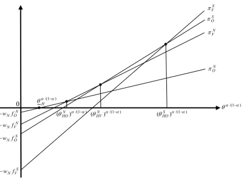
We next consider a sector with high headquarter intensityη, such thatβ∗(η)> βN_V . We refer to it as a high-tech sector. A sector of this type is represented by η=ηH in Figure 2. In this sector profits are increasing in the fraction of revenue β_k, as shown by the arrows in thefigure. In a high-tech sector the marginal product of headquarter services is high, making underinvestment byfinal-good producers especially costly. As a result, ex-ante maximization of value favors integration over outsourcing as long as there are no other differences in the benefits and costs of alternative organizational forms. In particular, equation (7) implies that in a high-tech sectorψ_V(η)> ψ_O(η)for

=N, S. Namely, in every country the slope of the profit function is steeper when the

firm is vertically integrated than when it outsources components.

Now compare the slope of the profit function of an integrated firm that produces components in the North with the slope of the profit function of afirm that outsources its components in the South, where the slope is measured relative to theθα/(1−α) axis (see Figure 4). The integrated firm has the advantage of being able to save a positive fractionδN of output when it severs its ties with the operator of the production facility of components, while the outsourcingfirm saves no output at all when it severs its ties with the arm’s-length supplier of components. On the other hand, the integratedfirm faces higher production costs, because the wage rate is higher in the North. For these reasons the profit function of thefirm outsourcing in the South can be steeper orflatter than the profit function of the integratedfirm in the North, depending on whether δN

0 N O Nf w − S V Nf w − S O π ) 1 /( α α θ − ) 1 /( α α θ − H ) 1 /( ) (θN α −α HO N O π S O Nf w − N V Nf w − ) 1 /( ) (θN α −α HV (θHOS )α/(1−α) N V π S V π

Figure 4: Equilibrium in the Hi-Tech Sector

is small or large, respectively, relative to the wage differential. That is, ψS_O(η) can be larger or smaller thanψNV (η).

First consider the case in which the wage differential is large relative toδN, so that

ψSO(η)> ψ N

V(η).17 Under these circumstances

ψSV(η)> ψ S O(η)> ψ N V(η)> ψ N O(η). (14)

Given the ordering in (3) and (14), the order of the intercepts and the slopes of the profit functions are as depicted in Figure 4. The intersection point of πN

O with the horizontal axis is to the left of the intersection point of this profit line with πN

V, the latter intersection point is to the left of the intersection point ofπNV with πSO, and this

17_{This condition is satisfied if and only if}

µ wN wS ¶1−η > n 1₋αhβNVη+ ³ 1₋βNV ´ (1₋η)io (1−α)/α³ βNV ´η³ 1₋βNV ´1−η {1₋α[βη+ (1₋β) (1₋η)]_}(1−α)/αβη(1₋β)1−η

(see (7)). This inequality always holds in low-tech sectors (in which the right-hand-side is smaller than one), but may not hold in high-tech sectors (in which the right-hand-side is larger than one).

last intersection point is to the left of the intersection point of πS

O with πSV. We take this situation to be the generic case of a high-tech sector. In this case all firms with productivity belowθ_H exit the industry, those with productivity betweenθ_H and θN_HO

outsource in the North, those with productivity between θN_HO and θN_HV integrate in the North, those with productivity betweenθNHV andθ

S

HO outsource in the South, and those with productivity above θS_HO integrate in the South (engage in vertical FDI). It is easy to see that either one of the first three organizational forms may not exist in equilibrium, but that the last one always exists. That is, there always exist high-productivityfinal-good producers who choose to manufacture components in the South. The cutoffs depicted in Figure 4 are given by

θ_H =X(α−µ)/αhwNfON ψNO(η) i(1−α)/α , θN_HO =X(α−µ)/α · wN_(fN V−fON) ψNV(η)−ψNO(η) ¸(1−α)/α , θN_HV =X(α−µ)/α · wN_(fS O−fVN) ψS_O(η)−ψN_V(η) ¸(1−α)/α θS_HO =X(α−µ)/α · wN_(fS V−fOS) ψS V(η)−ψSO(η) ¸(1−α)/α .                        (15)

We can also use the free entry condition (11) to derive an equation that is analogous to (13). This equation together with (15) can then be used to solve for the cutoffs and the consumption index X.18

Next consider cases in which ψSO(η) < ψ N

V (η), i.e., the profit function from in-tegration in the North has a larger slope than the profit function from outsourcing

18_{Suppose instead that thefixed costs of outsourcing are higher than thefixed costs of integration}

in each one of the countries, but that thefixed costs of integration in the South are higher than the fixed costs of outsourcing in the North. Then, in a high-tech sector integration dominates outsourcing in each one of the countries, because thefixed costs of integration are lower than the fixed costs of outsourcing and the profit function of an integrated firm is steeper than the profit function of an outsourcingfirm. As a result, nofirm outsources. Amongst thefinal-good producers who stay in the industry, low-productivityfirms integrate in the North while high-productivityfirms integrate in the South. The reversal of the ordering of thefixed costs also affects the sorting offirms by organizational form in low-tech sectors. Now, in a low-tech sector integration may dominate outsourcing at certain productivity levels. In particular, the least productivefinal-good producers who stay in the industry may integrate in the North, some more productive firms may outsource in the North, still higher-productivityfirms may integrate in the South, and the most productivefirms outsource in the South.

in the South. This happens when the wage differential is small relative to δN.19 _In

this event the ordering in (14) is not preserved. There are two possibilities: either

ψS_V(η)> ψN_V(η)> ψS_O(η)> ψN_O(η) orψN_V(η)> ψS_V(η)> ψ_OS(η)> ψN_O(η).20 _{The former}

case arises when the wage differential is small relative to δN, but not so small relative to the difference between δN and δS. On the other hand, the latter case arises when the wage differential is small even relative to the difference betweenδN and δS. If, for example, the wage rates are almost identical, then the fact that an integrated fi nal-good producer in the North can save a larger fraction of output than an integrated

final-good producer in the South can when both sever their ties with the components manufacturers, makes the former’s profits more sensitive to productivity changes than the latter’s. As a result, ψNV(η)> ψ

S V(η).

In thefirst case, when ψS_V(η)> ψN_V(η)> ψS_O(η)> ψN_O(η), integration in the North dominates outsourcing in the South, because it has lower fixed costs of organization and higher profits per unit productivity θ. Namely, the profit line πN

V in Figure 4 has a higher intercept and a larger slope than πS

O. In this event no firm chooses to outsource in the South, and the model predicts that – amongst thefirms that do not exit the industry – low-productivityfirms outsource in the North, high-productivity

firms integrate in the South, and firms with intermediate productivity levels integrate in the North.

In the second case, when ψN_V(η) > ψS_V(η) > ψS_O(η) > ψN_O(η), integration in the North dominates both outsourcing in the South and integration in the South. As a result, at most two organizational forms survive in equilibrium: low-productivityfirms that outsource in the North and high-productivityfirms that integrate in the North.

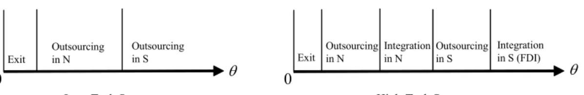
We have characterized the organizational forms in low-tech and high-tech sectors. The choice of organizational forms byfirms with different productivity levels is depicted in Figure 5. This figure describes the generic cases. First, low-tech firms do not integrate into the production of components; low-productivity firms outsource them in the North while high-productivity firms outsource them in the South. The least

19_Namely, µ wN wS ¶1−η < n 1₋αhβN_Vη+³1₋βN_V´(1₋η)io(1−α)/α³βN_V´η³1₋βN_V´1−η {1₋α[βη+ (1₋β) (1₋η)]_}(1−α)/αβη(1₋β)1−η . 20_{Note thatψ}S

0 θ Outsourcing in N Outsourcing in S Exit 0 θ Outsourcing in N Outsourcing in S Exit Integration in S (FDI) Integration in N

Low-Tech Sector High-Tech Sector

Figure 5: Organizational Forms

productivefirms exit. On the other hand, integration always takes place in high-tech sectors. The most productivefirms integrate in the South via foreign direct investment while somewhat less productive firms outsource in the South. Firms with even lower productivity acquire components in the North. Amongst those, the more productive

firms integrate while the less productive outsource. The least productivity firms exit. Note that survivingfirms with the lowest productivity outsource in the North in both low-tech and high-tech sectors. And more generally, less productive firms acquire components in the North while more productivefirms acquire them in the South.

This sorting pattern differs from the sorting pattern derived by Grossman and Helpman (2002b) for organizational structures that use managerial incentives à la Holmstrom and Milgrom (1994).21 _{Contrary to our results, in their model}

surviv-ing low-productivity firms acquire components in the South. Within this group less-productivefirms outsource while more-productivityfirms integrate via FDI. While no one outsources inputs in the North, there exist modestly-high productive firms that integrate in the North. However, the most-productive firms, like the least-productive

firms, outsource in the South.

Evidently, the two models predict very different sorting patterns. It would be interesting and useful to gauge which pattern betterfits reality. There exists, however, no evidence that bears directly on this question. And it is hard to see how to test these predictions with the available data.

It also is important to bear in mind that the most suitable theory of the firm can differ across sectors. Namely, the Grossman-Hart property-rights approach may be

21_{They did not distinguish between low- and high-tech sectors, however, although one can interpret}

their production technology as havingη= 0, i.e., a zero output elasticity with respect to headquarter services. For this reason a comparison of the cross-section variation of organizational forms that is based on the low-tech high-tech distinction cannot be made with their work.

most suitable for some industries while the Holmstrom-Milgrom managerial-incentives approach may be most suitable for others.22 _{This possibility would complicate every}

empirical analysis that tries to explain the cross-sectional variation in organizational forms. An appreciation of this possibility also raises an interesting theoretical question, the answer to which may help to design an empirical strategy: How do companies in a particular industry choose between the property-rights approach and the managerial-incentives approach in the organization of their activities? Or, more broadly, how do they choose endogenously the structure of ownership and incentives? To sort out the determinants of the organizational forms of industries together with an endogenous choice of incentives schemes and the structure of ownership is a major challenge for future research.

5

Prevalence of Organizational Forms

Our analysis has so far focused on the sorting patterns of firms into different organi-zational forms: outsourcing in the North, integration in the North, outsourcing in the South, and integration in the South. How prevalent are these organizational forms? And what determines their relative prevalence in different industries? To answer these questions we need a measure of prevalence. We choose the relative fractions of the varieties offinal goods that are produced under these organizational forms as our mea-sures of relative prevalence. We show in the appendix, however, that our results do not depend on this choice, in the sense that other measures – such as market shares of final goods – deliver similar results.23

Following Melitz (2002) and Helpman, Melitz and Yeaple (2002), we choose G(θ)

to be a Pareto distribution with shapek.24 _{That is,}

G(θ) = 1₋ µ b θ ¶k for θ _≥b >0. (16) Under this assumption, the distribution of sales is also Pareto, a feature consistent with

22_{The empowerment of workers may also be an important determinant of the structure of firms.}

Puga and Trefler (2002) and Marin and Verdier (2003) have developed general equilibrium frameworks in which everyfirm chooses endogenously the structure of authority within the organization.

23_{See also Grossman and Helpman (2002b) for this point.}

the evidence.25 _{We use this distribution in the following analysis. As in the previous}

section, we focus on low- and high-tech sectors.

5.1

Low-tech sector

Recall that in a low-tech sector nofirm integrates into the production of intermediates, because the outsourcing of components delivers higher operating profits. In the generic case depicted in Figure 3, final-good producers with productivity below θL exit the industry, those with productivity betweenθ_LandθN_LOoutsource in the North, andfirms with higher productivity levels outsource in the South. Denote byσ_LO the fraction of

active final-good producers who outsource in country . Then in the generic low-tech sectorσS

LO =

£

1₋G¡θN_LO¢¤/[1₋G(θ_L)]andσN

LO = 1−σSLO. The Pareto distribution (16) then implies that σS

LO =

¡

θ_L/θN_LO¢k. Substituting (12) into this expression, we obtain σS_LO = · ψS_O(η)₋ψN_O(η) ψN_O(η) fN O fS O−fON ¸k(1−α)/α . (17)

First consider the effect of the Southern wage rate. A lower wage in the South raises the profitability of outsourcing in the South, by increasing ψS_O(η). In this event, (17) implies a rise in the share of final-good producers that outsource components in the South. It can also be shown that the threshold productivity levelθL is higher the lower the wage rate in the South. The lower wage raises profits from outsourcing components in the South, therefore shifting upwards the profit line πS

O in Figure 3. But this raises the expected profits of entrants into the industry, attracting new producers of final goods. As a result the real consumption indexX rises, shifting down both profit lines. The final outcome is a higher threshold θL, which implies that a larger fraction of thefinal-good producers who enter the industry exit upon learning their productivity level. Evidently, the lower wage in the South induces a reorganization among thefi nal-good producers in the North that leads them to rely more on arm’s-length imports of components.

The model can easily be extended to incorporate transport costs for intermediate inputs. If the shipment of components is subjected to melting-iceberg-type transport costs, then a fall in transport costs is very similar to a decline in the Southern wage rate. It follows that lower transport costs lead to exit of a larger fraction of entrants

(as in Melitz, 2002) and to a larger fraction of final-good producers who outsource components in the South.26

Second, we have assumed for simplicity that an outsourcing final-good producer appropriates a fractionβ of the surplus from its relationship with the supplier of parts, irrespective of whether the supplier is in the North or in the South. Imagine, however, a situation in which this fraction can differ between the countries, and that thefinal-good producer now gets a smaller fraction of the surplus from outsourcing in the South (but still higher thanβ∗(η), so that the condition of a low-tech sector remains valid). Such a decline in the bargaining power in the South raises the profitability of outsourcing in the South via an increase inψS_O(η). As a result, the fraction of final-good producers who outsource in the South rises.

Third, consider an increase in the dispersion of productivity, which is represented by a decline ofk. Since the expression in the brackets on the right hand side of (17) represents the ratio of the cutoffs θ_L/θN_LO and this ratio is smaller than one, it follows that a rise in dispersion raises the fraction of final-good producers who outsource in the South.27

Finally, note that the degree of a sector’s headquarter intensity affects its relative prevalence of outsourcing in the two countries. SinceψS_O(η)/ψN_O(η) =¡wN_/wS¢(1−η)α/(1−α) (see (7)), it follows that among the low-tech sectors those whose technology is more intensive in headquarter services outsource relatively less in the South. Intuitively, the less important are components in the production of the final good, the less important are the cost savings from outsourcing components in the South as compared to the higherfixed organizational costs of this activity.

5.2

High-tech sector

In the generic case of the high-tech sector, there are four organizational forms, ordered from low- to high-productivity firms: outsourcing in the North, integration in the North, outsourcing in the South and integration in the South (see Figures 4 and 5). We denote by σ_Hk the share of products that are supplied with the organizational

26_{In the U.S. manufacturing sector, the sum of tariffduties and freight costs has steadily fallen from}

11.3% of the Customs value of imports in 1974 to 5.1% in 2001. We computed thesefigures from data available on Robert Feenstra’s website.

27_{This is similar, in terms of the mechanism at work, to the finding in Melitz (2002) that more}

dispersion raises the share of exportingfirms in domestic output, and thefinding in Helpman, Melitz and Yeaple (2002) that more dispersion raises horizontal FDI relative to exports.

form (k, ), where k is the ownership structure and is the location of production of components. Using the Pareto distribution (16) and the cutoffs (15), these shares are

σN HO = 1− h_ψN V(η)−ψ N O(η) ψNO(η) f_ON fN V−fON ik(1−α)/α , σN HV = h_ψN V(η)−ψNO(η) ψN O(η) fN O fN V−fON ik(1−α)/α −hψSO(η)−ψNV(η) ψN O(η) fN O fS O−fVN ik(1−α)/α , σS HO = h_ψS O(η)−ψNV(η) ψNO(η) fN O fS O−fVN ik(1−α)/α −hψSV(η)−ψSO(η) ψNO(η) fN O fS V−fOS ik(1−α)/α , σS HV = h_ψS V(η)−ψSO(η) ψN O(η) fN O fS V−fOS ik(1−α)/α .                  (18)

We again first consider a lowering of the wage rate in the South. Lower wages in the South raise the profitability of foreign integration and foreign outsourcing. In particular, (7) implies that ψS_V (η) and ψS_O(η) increase while ψN_V (η) and ψN_O(η) do not change. It then follows from (18) thatσN

HO does not change. Namely, the share of products that are supplied byfinal-good producers who outsource in the North remains the same. On the other hand, the share of products supplied by vertically integrated producers in the North,σN

HV, declines. The reason is that low-productivity firms that outsource in the North are too far from productivity levels that make the acquisition of inputs in the South profitable. As a result, small changes in the profitability of importing inputs, be it through arm’s-length transactions or via FDI, does not make the purchase of inputs in the South attractive to these firms. On the other hand, amongst the integrated producers in the North the most productive are indifferent between integration in the North and outsourcing in the South. Therefore, for these

firms a decline in the South’s wage rate tilts the balance in favor of outsourcing in the South. For this reason the share of final-good producers who outsource in the South, σS

HO, rises.28 Finally, the share of firms that integrate in the South, σSHV, also rises. Evidently, lower labor costs in the South induce a reorganization that favors the acquisition of components in the South, but it has a disproportionately large effect on outsourcing as compared to FDI. At the same time the unfavorable effect on the acquisition of inputs in the North falls disproportionately on integration. It follows that outsourcing rises overall relative to integration.

A fall in transport costs of intermediate inputs has the same effects as a fall inwS. It is interesting to note that the recent trends described in the introduction are in line with

28_{This is easy to see from (18) by noting that the ratio ψ}S V(η)/ψ

S

O(η)is independent of the wage ratewS_.

the model’s predictions about falling costs of doing business in the South. Feenstra and Hanson (1996) point out that transport costs have declined and foreign assembly has increased both in-house and at arm’s length. Furthermore, Table 1 suggested that the growth of foreign outsourcing might have outpaced that of foreign direct investment. Finally, as predicted by the model, U.S. domestic outsourcing seems to have increased relative to U.S. domestic integration at a time of falling trade barriers (see Figure 1).29

Second, consider the effect of δ , the share of output that a final-good producer who is integrated in country retains in case it severs its ties with the operator of the production unit of components. We start with an increase in this share in the South. This improves the outside option of an integrated producer in the South in its bar-gaining with the operator of the production unit of components. The better outside option translates into higher effective bargaining power, as measured by βS_V. As is evident from (7), a higherβS_V raises ψS_V (η) without affecting the slopes of other profit functions. Equations (18) then imply that the shares of products that are supplied byfinal-good producers who acquire components in the North, either via outsourcing or integration, do not change. In this event, the fraction of final goods that use im-ported components does not change too, except that amongst those who use imim-ported components the share of outsourcingfirms declines while the share of integratedfirms rises.

An increase inδN raises the effective bargaining power of an integrated producer in the North. As a result, integration in the North becomes more profitable and the slope

ψNV (η) rises; the other slopes do not change. It then follows from (18) that the share of final-good producers who outsource in the North declines, the share of integrated

firms in the North rises, the share of outsourcing firms in the South declines, and the share of integratedfirms in the South does not change. The interesting implication is that the improvement in the attractiveness of domestic integration changes the relative prevalence of foreign outsourcing relative to FDI in favor of the latter.

Third, consider an increase in the primitive bargaining power β. It can be shown that it reduces the ratios ψS_V (η)/ψ_O(η) and ψN_V (η)/ψ_O(η) for = N, S as well as

ψNV (η)/ψ S

V (η). The reason is that an increase inβ shifts the bargaining power in favor of thefinal-good producer, regardless of ownership structure. As a result, thefinal-good

29_{As in the a low-tech sector, lower labor costs in the South or lower transport costs of intermediates}

increase the cutoffproductivity level below whichfinal-good producers exit the industry in a high-tech sector. This implies a higher proportion of exitingfirms.

producerfinds it relatively more profitable to outsource. In this event the share offi nal-good producers who outsource components rises in the North as well as in the South. On the other hand, the share of final-good producers who integrate declines in the North as well as in the South. Moreover, the fraction offirms that import components rises. That is, the rise in the share of outsourcingfirms in the South is larger than the fall in the share of firms that engage in foreign direct investment. It follows that an increase in thefinal-good producer’s bargaining power biases the acquisition of inputs towards imports on the one hand and towards outsourcing as opposed to integration on the other.

Fourth, we examine an increase in the degree of dispersion of the distribution of productivity, as represented by a fall in the shape parameter k. It is evident from (18) that a decline in k reduces the share of firms that outsource in the North and increases the share of firms that integrate in the South. The effect on the share of

firms that integrate in the North or outsource in the South is ambiguous, however. Yet the share of final-good producers who import components from the South rises, and so does the prevalence of FDI relative to outsourcing in the South (i.e., the ratio

σS

HV/σSHO) and the prevalence of integration relative to outsourcing in the North (i.e., the ratioσN

HV/σNHO).

Finally, we consider variations in headquarter intensity. In sectors with higher head-quarter intensity domestic outsourcing is favored relative to foreign outsourcing and in-tegration is favored relative to outsourcing. That is,ψN_O(η)/ψS_O(η)andψ_V (η)/ψ_O(η)

for =N, S are higher in sectors with larger values ofη.30 Equations (18) then imply that the share of final-good producers who outsource in the North falls with η while the share offinal-good producers who integrate in the North rises. Moreover, the sum of these two shares goes up, implying that a larger η reduces the fraction of firms that import components. As for the composition of imported components, we cannot sign the effects of η on the share of firms that import from integrated subsidiaries. Nevertheless, (18) implies that the ratio σS

HV/σSHO rises and, hence, that σSHO falls. Namely, FDI becomes more prevalent relative to arm’s-length imports. It follows that in a cross-section of high-tech sectors the relative prevalence of integration rises and the relative prevalence of outsourcing falls with headquarter intensity. This prediction is in line with the findings of Antràs (2002a), who shows that in a panel of 23

facturing industries and four years of data, the share of intra-firm imports in total U.S. imports is significantly higher, the higher the R&D intensity of the industry.31

6

Concluding Comments

We have developed a theoretical framework for studying global sourcing strategies. In our model, heterogeneous final-good producers choose organizational forms. That is, they choose ownership structures and locations for the production of intermediate inputs. Headquarter services are always produced in the home country (the North). Intermediate inputs can be produced at home or in the low-wage South, and the pro-duction of intermediates can be owned by thefinal-good producer or by an independent supplier. When afinal-good producer owns the production unit of components and this unit is located in the North, the organizational form is one of standard vertical inte-gration. When, on the other hand, the production unit of the intermediate inputs is located in the South, the organizational form is one of integration with vertical foreign direct investment. This type of FDI generates intra-firm international trade. A fi nal-good producer who does not integrate into the production of components outsources them to independent suppliers. Such afinal-good producer can outsource in the home country or in the South. In the latter case outsourcing generates international trade at arm’s length.

Final-good producers and operators of components production units make relationship-specific investments which are governed by imperfect contracts. In choosing between a domestic and a foreign supplier of parts, a final-good producer trades off the benefits of lower variable costs in the South against the benefits of lower fixed costs in the North. On the other hand, in choosing between vertical integration and outsourcing in one of the countries, thefinal-good producer trades offthe benefits of ownership from vertical integration against the benefits of better incentives for the supplier of parts un-der outsourcing. These tradeoffs inducefirms with different productivity levels to sort by organizational form. We show that the equilibrium sorting patterns depend on the wage differential between the North and the South, on the ownership advantage in each

31_{Controlling for several industry characteristics, Antràs (2002a) finds that a 1% increase in the}

ratio of industry R&D expenditures over industry sales leads to a 0.42% increase in the fraction of that industry’s U.S. imports that are transacted withinfirm boundaries. The effect is significant at the 1% significance level.

one of the countries (as measured by the fraction of output that afinal-good producer can recoup in the event of a breakup of his relationship with an integrated supplier of components), on the distribution of the bargaining power betweenfinal-good producers and operators of components production facilities, and on the headquarter intensity of the production process.

A key result is that high-productivity firms acquire intermediate inputs in the South while low-productivityfirms acquire them in the North. Amongst thefinal-good producers who acquire inputs in the same country the low-productivityfirms outsource while the high-productivity firms integrate. In sectors with a very low intensity of headquarter services nofirm integrates; low-productivityfirms outsource at home while high-productivityfirms outsource abroad.

We construct industry equilibria and use them to characterize the relative preva-lence of alternative organizational forms. By relative prevapreva-lence we mean the fraction of final-good producers who choose a particular organizational form. Relative preva-lence depends on all the features of an industry that affect the sorting pattern of its

firms into various organizational forms. In addition, it depends on the degree of disper-sion of productivity across the industry’sfirms. Using these relationships, we describe how differences in industry characteristics affect the relative prevalence of various or-ganizational forms.

Two results stand out. First, sectors with more dispersion of productivity rely more on imported inputs. And moreover, amongst the headquarter-intensivefinal-good producers who acquire inputs in a particular country, the number of integratedfirms is higher relative to the number of outsourcing firms the more dispersed is productivity within the sector. Second, the higher a sector’s headquarter intensity, the less it relies on imported intermediate inputs. And amongst the headquarter-intensive final-good producers who acquire inputs in a particular country, the number of integrated firms is higher relative to the number of outsourcingfirms the more headquarter intensive is the sector.

Our model has also interesting implications for the effects of a widening of the wage gap between the North and the South, or a reduction of the trading costs of intermediate inputs (both changes produce similar outcomes). As one would expect, reducing the relative cost of foreign sourcing raises the prevalence of organizational forms that rely on imported inputs. Importantly, however, such shifts in costs also affect the relative