Volume 125 – No.8, September 2015
A New Shear Wave Speed Estimation Method for Shear
Wave Elasticity Imaging
Mohammed A. Hassan
Dept of Biomedical Engineering, Faculty of Engineering, Helwan University, EgyptNancy M. Salem
Dept of Biomedical Engineering, Faculty of Engineering, Helwan University, EgyptMohamed I. El-Adawy
Dept of Electronics, Communications, and Computer Engineering, Facultyof Engineering, Helwan University, Egypt
ABSTRACT
In this paper, a novel method to estimate the shear wave speed is proposed. This method is a modified version of the lateral Time to Peak (TTP) method that estimates the induced shear wave speed. Lateral TTP algorithm finds the instance at which the maximum displacement is detected at each lateral location under examination at a certain depth. In the proposed algorithm each temporal displacement data is enhanced by fitting a Gaussian distribution into it prior to finding instance at which the peak displacement detected. This algorithm is validated on tracked displacements generated from a finite-element model (FEM) that simulates the dynamic response of tissues to acoustic radiation forces. The proposed algorithm reveals a reconstruction of materials having shear modulus of 1.33 kPa as 1.28±0.05 kPa, 2.835 kPa as 2.84±0.23 kPa, and 8 kPa as 7.94±0.58 kPa. However, lateral TTP method revealed a reconstruction of materials having shear modulus of 1.33 kPa as of 1.31 ± 0.03 kPa, and 8 kPa as 2.77 ± 0.08. Finally, Gaussian fitting can be used to enhance results obtained from Lateral TTP algorithm by providing a more accurate reconstruction of materials shear modulus.
Keywords
Shear wave elasticity imaging, acoustic radiation force, finite element method, shear wave speed estimation, lateral Time to Peak, Gaussian fitting
1.
INTRODUCTION
Ancient Egyptians used tissue palpation as a fundamental medical diagnosis method, this method is used commonly and effectively in diagnosis until now. However, this qualitatively method can only be used for legions that are superficial, large, and that have a big stiffness difference compared to their surrounding tissues. Remote palpation techniques were developed to overcome these drawbacks and provide non-invasive means of estimating the biomechanical attributes of tissues especially the elastic (Young’s) modulus even for deep and small tissues. These remote palpation techniques are called Elastography techniques [1-3].
Many researchers used Elastography techniques and proved that generated elastograms may not just differentiate effectively between benign and malignant lesions, but they are capable of differentiating between subtypes of malignancy [4, 5]. In some cases elastograms are better than conventional diagnostic B-mode ultrasound images [6], diagnosis of atherosclerosis [7], detection and grading of deep vein thrombosis [8], imaging of skin pathologies [9] and evaluation of myocardial stiffness [10]. Elastography methods are categorized according to different criteria such as excitation source, and/or being quantitative, or qualitative methods.
Qualitative, i.e., quasi-static, free hand, and Acoustic radiation Force on-axis Imaging (ARFI) methods, produce displacement or strain images. On the other hand quantitative methods such as Fibroscan, Super Sonic Imaging (SSI), and Shear Wave Elasticity Imaging (SWEI) methods can be used to measure tissue stiffness (i.e. the elastic (Young’s) modulus) [1, 11-13].
In this paper, a simulation model of the dynamic response of soft tissue to a transient acoustic radiation force impulse (ARFI) excitation using a commercially available, diagnostic, ultrasound transducer is introduced. Then a novel method to estimate the shear wave speed is proposed. This paper is organized as follows. Introduction about elastography, SWEI, and shear wave speed estimation methods are presented in the introduction section. Methodology section demonstrates shear wave generation and imaging method used in our experiment and demonstrates the proposed method. Finally, results, discussion, and conclusion sections is give at the end of the paper.
2.
SHEAR WAVE ELASTICITY
IMAGING
2.1
Acoustic Radiation Force
Acoustic radiation force (ARF) is a phenomenon associated with acoustic wave’s propagation in attenuating media. Attenuation includes both the scattering and absorption of the acoustic wave. As shown by Nyborg [14], under plane wave assumptions and by neglecting scattering where the majority of the attenuation of ultrasound arises from absorption [15], acoustic radiation force (F) can be related to the acoustic absorption (), speed of sound (c) of the tissue, and the temporal average intensity of the acoustic beam (I) by:
𝐹 =2𝛼𝐼𝑐 (1) where F [kg/(s2cm2)] is in the form of a body force per unit volume, c [m/s] is the sound speed, [Np/cm] is the absorption coefficient of the tissue which is frequency dependent phenomenon, and I [W/cm2] is the temporal average intensity at that spatial location. This body forces can be induced in the tissue within the geometric shadow of the active aperture of the transducer having a peak value near the focal point.
The geometrical distribution of this force is dependent on the acoustic parameters of the transmitter along with the speed of sound, and the transducer focal configuration, which can be characterized by the f-number (F/#) of the system:
𝐹 # = 𝑧
Volume 125 – No.8, September 2015
where z is the acoustic focal length, and a is the active aperture width.
2.2
Shear Wave Generation
Sarvazyan et al. have proved that a short-duration focused excitation of a commercially available ultrasound transducer can be used to generate acoustic radiation body forces, which induce tissue displacement centered on the focal region. These displacements propagate through the tissue in the form of shear waves perpendicular to the direction of excitation force (i.e. parallel to transducer surface). This wave can be detected, either by optical coherence tomography, magnetic resonance imaging (MRI), or ultrasound imaging techniques and displayed as an image, their speed is then used to estimate the elasticity of the tissue [16].
Shear wave speed velocity is related to tissue stiffness (i.e. shear modulus, and elastic modulus) using the following equations assuming a pure elastic, homogenous medium [17]:
𝑐𝑇 = 𝜇𝜌
(3)
𝜇 = 𝐸
2(1+𝑣) (4)
where cT[m/s] is shear wave speed velocity, [Pa] is the shear modulus, E[Pa] is the elastic modulus, [kg/m3] is the density, and is the Poisson’s ratio.
2.3
Shear Wave Estimation
Shear wave is monitored outside the region of excitation (ROE) within focal zone [17-19]. Many researchers have quantified tissue stiffness from shear wave speed (SWS) estimation from dynamic displacement data. SWS estimation from the algebraic inversion of the second-order Helmholtz differential equation has been successfully applied to MRI data [20, 21] but with limited success to ultrasound [22-24] due to the noisy nature of ultrasound displacement estimates. Another technique involves estimation of either the spatial or temporal frequency of monochromatic shear waves, given a priori knowledge of its counterpart [25-27]. By assuming a fixed direction of shear wave propagation, and a given arrival time at multiple spatial locations, then SWS can be estimated using linear regression algorithms. This approach is called time-of-flight (TOF) approach, that has been successfully applied to ultrasound tracked shear wave displacement data [28-31].
3.
METHODOLOGY
Finite element models (FEM) were developed to simulate the effect of the induction of a transient duration (<100 s) and spatially localized impulsive acoustic radiation body forces in tissue. A FieldII [32] simulation software is used to calculate and calibrate the pressure field generated from a commercially available, diagnostic, ultrasound transducer and to image the induced displacements in the tissue at different spatial location at different times after excitation. The mechanical response of the tissue to ARF body forces is simulated using LS-DYNA3D [33] FEM solver software, and LS-PREPOST [34] program [17, 35].
3.1
FEM Mesh Generation
The FEM model presented in this paper is similar to FEM model described by Palmeri et al . [17] in which, a three dimensional, rectangular, uniform distributed solid mesh was assembled using linear, elastic, and eight nodded brick elements using HyperMesh [36] program. This mesh represents a soft tissue extends to 7.5 mm, 25 mm, and 35 mm
in elevation, axial, and lateral directions respectively with node spacing of 0.2 mm. There are 842688 elements and 876681 nodes within the model. The bottom surface of the model opposing the transducer was fully constrained; the top surface (transducer surface) was allowed to move only within the plane perpendicular to axial direction. All other surfaces of the model have full degrees of freedom. This model has a density of 1.060 g/cm3, poisons ratio of 0.499, and an attenuation of 0.7 dB/cm/MHz.
3.2
Pushing Beam Intensity Generation
and Calibration
In our experiments, a model of Siemens SONOLINE ElegraTM ultrasound scanner VF10-5 linear array transducer with center frequency of 6.67 MHz was built using FieldII program. The transducer is laterally focused at 20 mm with F/1.3 focal configuration, and focused at 20 mm in elevation with F/3.8 focal configuration. This transducer is used to excite the tissue with a high intensity low duration pushing beam and generate a displacement within tissue. The aperture (using 96 element) was unapodized with longer pulse duration 43 s (e.g. 300 cycles at 6.67 MHz). The excitation voltage of the transducer elements were calibrated to generate a spatial peak temporal average intensity (Ispta) of 1000 W/cm2 using FieldII program, Table 1 summarize excitation parameters. The spatial location of maximum intensity is located proximal than focal point due to acoustic attenuation of the tissue. Only nodes that have intensity greater than 1% of its maximum generated intensity value is used to generate ARF to reduce the computational time of the model.
3.3
FEM Implementation and
Post-processing
ARF forces is then calculated from Eq. 1 and directed to the axial direction and converted to nodal point loads by concentrating the body force contributions over an element volume. The response of the tissue model to transient acoustic radiation body forces as dynamic displacements was obtained using the commercially available FEM package LS-DYNA3D software. FEM generated displacements are obtained at each pulse repetition time (PRT = 0.1ms) instances for with a total simulation time equals 5 ms using an explicit, time-domain, and integration method. Single-point quadrature was performed with hourglassing control to avoid element locking and to reduce numerical artifacts [17, 35, 37], in addition to LS-PREPOST program and custom-written MATLAB code. Three types of tissues have been examined in this experiment having a shear moduli of 1.33, 2.835, and 8 kPa in three different implementations.
Figure 1 illustrates shear wave propagation in the central elevation plane at 0.6 ms, 1 ms, and 2.2 ms in 8 kPa shear modulus simulated tissue, as normalized displacement profiles. Normalized displacement profiles are illustrated as gray levels (i.e. the brightest pixels represent the maximum displacement and vise versa.
Ax ia l (m m ) Ax ia l (m m ) Lateral (mm) Lateral (mm) (A) (B)
Volume 125 – No.8, September 2015 Ax ia l (m m ) Lateral (mm) (C)
Fig 1. Shear wave location in central elevation plane at A) 0.6 ms, B) 1 ms, and (C) 2.2 ms in 8 kPa shear modulus of untracked FEM generated displacements of simulated tissue. Shear wave location at any instance is displayed as
normalized displacement profiles. Normalized displacement profiles is illustrated as gray levels (i.e. the brightest pixels represent the maximum displacement and
vise versa.
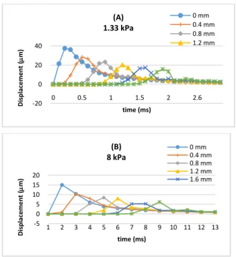
Figure 2 shows shear wave propagation at different lateral locations located at focal distance distal from the transducer in the central elevation plane of untracked FEM generated displacements of simulated tissue having shear modulus of 1.33 kPa, and 8 kPa.
Figure 2. Shear wave propagation at different lateral lines located at focal distance distal from the transducer at
central elevation plane of untracked FEM generated displacements of simulated tissue having shear modulus of
(A) 1.33 kPa, and (B) 8 kPa.
3.4
Tracking and Displacement
calculations
After FEM post-processing and dynamic displacement field data generation. A uniform scattering phantom having a randomly positioned scatterer points of equal echogenicity, the locations of these scatterer point are taken as initial reference undisplaced scatterer positions. A reference RF tracking lines at lateral lines spacing 0.2 mm starting from 0 mm were generated from these initial undispaced scatterer locations, Using FieldII ultrasound field simulation program [32] Table 1 summarize tracking parameters.
At each PRT instance repetition, the initial undispaced scatterers locations were then linearly interpolated from the displacement field vectors at each mesh point to generate displacement field vector displacement of scatterers at this instance. These interpolated displacement field vectors were used to reposition the scatterers. Tracking RF lines were generated at the same lateral locations as reference RF lines [38]. Induced tissue displacements due to ARFs are measured along each RF tracking lines by Loupas’ phase shift method on corresponding IQ data [39].
Table 1: Transducer configurations for the VF10-5 array
Excitation frequency (MHz) 6.7 Excitation duration (s) 45 Excitation F/# 1.3 Excitation focal depth (mm) 20 Lateral beam spacing (mm) 0.2 Tracking frequency (MHz) 6.7 Tracking transmit F/# 1 Tracking receive F/# 0.5 Elevation focus (mm) ~20 PRF of track lines (kHz) 10 Duration of tracking (ms) 5
3.5
Proposed Shear Wave Speed
Estimation Method
The proposed algorithm is a modified version of the Lateral TTP algorithm presented by Palmeri et al. [31]. It satisfies the assumptions of the TTP algorithm in which tissue is homogenous, wave propagates exclusively in the plane perpendicular to axial direction, and there is no dispersion in analyzed region. The analyzed region locates laterally outside the region of excitation (ROE) within the depth of field (DOF) that was defined by 8(F/#)2, where F/# and represent the
beam f-number, and wavelength of the pushing beam, respectively. The dimensionless excitation beam f-number
(F/#) was defined in Eq. 2. For each displacement, data from simulated ultrasonic tracking of the FEM modeled displacements were rearranged in three-dimensional array in which the axial position, lateral position, and time are they main dimension in order[40].
In the proposed algorithm, at each lateral location, the axial displacements are averaged over 0.5 mm for analysis, centered at the focus in this case 20 mm to reduce jitter/noise. The TTP displacement is estimated from the displacement signal through time data after this displacement signal fitting on 1D two Gaussian mixture distribution [41] without upsampling and low-pass interpolation as performed in the Lateral TTP algorithm.
For temporal displacement dataset, 1D two Gaussian mixture fitting is done by iteratively finding the parameters a1, b1,c1, a2, b2, and c2 that relates displacement dependent measurements to their corresponding temporal instance with least error using Eq. 5 [41].
𝑌 = 𝑎1𝑒 − 𝑋 −𝑏 1 𝑐1 2 + 𝑎2𝑒 − 𝑋 −𝑏 2 𝑐2 2 (5) -20 0 20 40 0 0.5 1 1.5 2 2.6 D isp la ce me nt ( m) time (ms) (A) 1.33 kPa 0 mm 0.4 mm 0.8 mm 1.2 mm -5 0 5 10 15 20 1 2 3 4 5 6 7 8 9 10 11 12 13 D isp la ce me nt ( m) time (ms) (B) 8 kPa 0 mm 0.4 mm 0.8 mm 1.2 mm 1.6 mm
Volume 125 – No.8, September 2015
Where a1, b1, and c1 are the amplitude, mean value, and
standard deviation of the first Gaussian mixture respectively while a2, b2, and c2 are the amplitude, mean value, and
standard deviation of the second Gaussian mixture respectively, Y is displacement measurements at X instances. No modifications are happened to linear regression implementation performed in the Lateral TTP algorithm. Regressions are not applied to lateral locations within ROE i.e. one excitation beam width defined by (F/#)* from excitation center and extended over lateral range where the peak displacements remained above 1 m. The inverse slopes of these regression lines, with goodness-of-fit metrics exceeding a threshold (R2 >0.8, 95% CI <0.2), represent the material’s local shear wave speeds. These specific goodness-of-fit metrics is applied to all of the datasets presented throughout this manuscript. The material’s shear modulus is then estimated using Eq. 3 [31].
4.
RESULTS
Theoretical values of shear wave speeds are 1.153, 1.683, and 2.828 m/s propagating in 1.33, 2.835, and 8 kPa shear moduli materials respectively. The proposed algorithm reveals estimation of SWS of same materials as 1.134±0.022, 1.686±0.036, and 2.817±0.052. The results represented with the mean ± one standard deviation shear wave speed estimates for 20 independent, simulated speckle realizations from FEM displacement data. The corresponding shear modulus estimates are 1.28±0.05, 2.84±0.23, and 7.94±0.58 kPa for 1.33, 2.835, and 8 kPa for shear moduli materials respectively. However, TTP method revealed results of 1.31±0.03, and 2.77±0.08 kPa for 1.33, 2.835 shear moduli materials respectively 20 independent, simulated speckle realizations from FEM displacement data [31, 33]. Table 2 summarizes results obtained by the proposed method and the lateral TTP method. It is clear that the proposed algorithm provides better results for 8 kPa shear modulus materials, and less accurate results for 1.33 shear modulus materials. The results obtained for 8 kPa shear modulus simulated materials using lateral TTP algorithm are not available.
Table 2: Comparison between results obtained from Lateral TTP and proposed algorithms Shear modulus (kPa) Theoretical SWS (m/s) Estimated shear modulus (kPa) Estimated SWS (m/s) Lateral TTP Proposed method Proposed method 1.33 1.153 1.31±0.03 1.28±0.05 1.134±0.022 2.835 1.683 2.77±0.08 2.84±0.23 1.686±0.036 8 2.828 N/A 7.94±0.58 2.817±0.052
5.
DISCUSSION
As reported in [31] that Lateral TTP reconstructions estimates shear moduli for materials ranging from 1.3–5 kPa with accuracy within 0.3 kPa, whereas stiffer shear moduli ranging from 10–16 kPa with accuracy in 1.0 kPa. The variance with stiffness because of fixed Pulse time that indicate the temporal sampling of displacement data given that shear wave velocity is proportional to the square root of shear modulus. Hence, SWS velocity is increased for stiffer materials with fixed sampling time will cause subsampling of displacement temporal data. Therefore, in Lateral TTP algorithm this effect my reveals a false detection of peak displacement. This effect has been overcomed by estimating the true location of peak as
the estimated mean value of fitted Gaussian estimate of displacement temporal data.
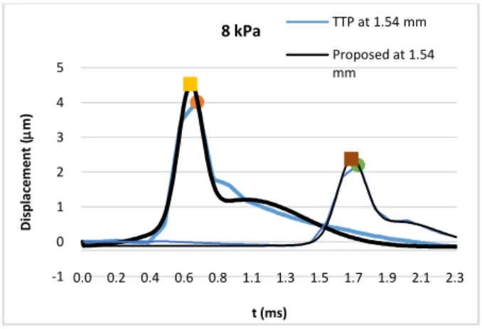
In the proposed method, the estimated instance of peak value is 0.66 ms at lateral location 1.54 mm while at the same lateral location the lateral TTP results in an estimated instance of peak value of 0.7 ms. At lateral position 1.76 mm, results from the lateral TTP method, and the proposed method are 1.7 ms, and 1.65 ms respectively.
Figure 3, Illustrates the location of estimated location of peak value using both TTP algorithm and proposed algorithm for a tracked FEM generated data using ultrasound for lateral locations 1.54 and 1.76 mm.
Figure 3. Estimated instance of peak values using both TTP algorithm and proposed.
6.
CONCLUSION
A new method to estimate shear wave speed is proposed. Gaussian fitting can be used to enhance temporal displacement data prior to finding instance at which the peak displacement detected. This step results in more accurate reconstruction of materials shear modulus. Although this modification revealed more accurate reconstruction of shear modulus than lateral TTP method for stiffer materials i.e. 2.835, and 8 kPa, it revealed less accurate reconstruction of 1.33 kPa materials’ shear modulus. The proposed algorithm requires more calculation time due to the iterative implementation of Gaussian fitting algorithm.
7.
REFERENCES
[1] P. N. T. Wells and H.-D. Liang, "Medical ultrasound: imaging of soft tissue strain and elasticity," Journal of the Royal Society Interface, vol. 8, pp. 1521-1549, 2011. [2] A. Sarvazyan, T. Hall, M. Urban, M. Fatemi, S.
Aglyamov, and B. Garra, "Elasticity imaging-an emerging branch of medical imaging. An overview," Curr. Med. Imaging Rev, vol. 7, pp. 255-282, 2011. [3] J. F. Greenleaf, M. Fatemi, and M. Insana, "Selected
methods for imaging elastic properties of biological tissues," Annual review of biomedical engineering, vol. 5, pp. 57-78, 2003.
[4] B. S. Garra, E. I. Cespedes, J. Ophir, S. R. Spratt, R. A. Zuurbier, C. M. Magnant, et al., "Elastography of breast lesions: initial clinical results," Radiology, vol. 202, pp. 79-86, 1997.
[5] E. S. Burnside, T. J. Hall, A. M. Sommer, G. K. Hesley, G. A. Sisney, W. E. Svensson, et al., "Differentiating benign from malignant solid breast masses with US strain Imaging1," Radiology, vol. 245, pp. 401-410, 2007. -1 0 1 2 3 4 5 0.0 0.2 0.4 0.6 0.8 1.1 1.3 1.5 1.7 1.9 2.1 2.3 D isp la ce me nt ( m) t (ms) 8 kPa TTP at 1.54 mm Proposed at 1.54 mm
Volume 125 – No.8, September 2015
[6] N. Miyanaga, H. Akaza, M. Yamakawa, T. Oikawa, N. Sekido, S. Hinotsu, et al., "Tissue elasticity imaging for diagnosis of prostate cancer: a preliminary report," International journal of urology, vol. 13, pp. 1514-1518, 2006.
[7] C. L. De Korte, G. Pasterkamp, A. F. Van Der Steen, H. A. Woutman, and N. Bom, "Characterization of plaque components with intravascular ultrasound elastography in human femoral and coronary arteries in vitro," Circulation, vol. 102, pp. 617-623, 2000.
[8] S. Emelianov, X. Chen, M. O’Donnell, B. Knipp, D. Myers, T. Wakefield, et al., "Triplex ultrasound: elasticity imaging to age deep venous thrombosis," Ultrasound in medicine & biology, vol. 28, pp. 757-767, 2002.
[9] M. Vogt and H. Ermert, "Development and evaluation of a high-frequency ultrasound-based system for in vivo strain imaging of the skin," Ultrasonics, Ferroelectrics and Frequency Control, IEEE Transactions on, vol. 52, pp. 375-385, 2005.
[10] K. Kaluzynski, X. Chen, S. Y. Emelianov, A. R. Skovoroda, and M. O'Donnell, "Strain rate imaging using two-dimensional speckle tracking," Ultrasonics, Ferroelectrics and Frequency Control, IEEE Transactions on, vol. 48, pp. 1111-1123, 2001.
[11] G. Treece, J. Lindop, L. Chen, J. Housden, R. Prager, and A. Gee, "Real-time quasi-static ultrasound elastography," Interface focus, vol. 1, pp. 540-552, 2011. [12] S. Rosenzweig, M. Palmeri, and K. Nightingale,
"Analysis of rapid multi-focal-zone ARFI imaging," Ultrasonics, Ferroelectrics, and Frequency Control, IEEE Transactions on, vol. 62, pp. 280-289, 2015.
[13] J. Foucher, E. Chanteloup, J. Vergniol, L. Castera, B. Le Bail, X. Adhoute, et al., "Diagnosis of cirrhosis by transient elastography (FibroScan): a prospective study," Gut, vol. 55, pp. 403-408, 2006.
[14] W. Nyborg, "Acoustic streaming," Physical acoustics, vol. 2, p. 265, 1965.
[15] P. G. Anderson, N. C. Rouze, and M. L. Palmeri, "Effect of Graphite Concentration on Shear-Wave Speed in Gelatin-Based Tissue-Mimicking Phantoms," Ultrasonic Imaging, vol. 33, pp. 134-142, Apr 2011.
[16] A. P. Sarvazyan, O. V. Rudenko, S. D. Swanson, J. B. Fowlkes, and S. Y. Emelianov, "Shear wave elasticity imaging: a new ultrasonic technology of medical diagnostics," Ultrasound in medicine & biology, vol. 24, pp. 1419-1435, 1998.
[17] M. L. Palmeri, A. C. Sharma, R. R. Bouchard, R. W. Nightingale, and K. R. Nightingale, "A finite-element method model of soft tissue response to impulsive acoustic radiation force," Ultrasonics, Ferroelectrics and Frequency Control, IEEE Transactions on, vol. 52, pp. 1699-1712, 2005.
[18] K. Nightingale, R. Bentley, and G. Trahey, "Observations of tissue response to acoustic radiation force: opportunities for imaging," Ultrasonic imaging, vol. 24, pp. 129-138, 2002.
[19] M. Palmeri, H. Feltovich, A. Homyk, L. Carlson, and T. Hall, "Evaluating the feasibility of acoustic radiation force impulse shear wave elasticity imaging of the
uterine cervix with an intracavity array: a simulation study," Ultrasonics, Ferroelectrics and Frequency Control, IEEE Transactions on, vol. 60, 2013.
[20] R. Sinkus, M. Tanter, T. Xydeas, S. Catheline, J. Bercoff, and M. Fink, "Viscoelastic shear properties of in vivo breast lesions measured by MR elastography," Magnetic resonance imaging, vol. 23, pp. 159-165, 2005. [21] T. E. Oliphant, A. Manduca, R. L. Ehman, and J. F. Greenleaf, "Complex‐valued stiffness reconstruction for magnetic resonance elastography by algebraic inversion of the differential equation," Magnetic resonance in Medicine, vol. 45, pp. 299-310, 2001.
[22] J. Bercoff, M. Tanter, and M. Fink, "Supersonic shear imaging: a new technique for soft tissue elasticity mapping," Ultrasonics, Ferroelectrics and Frequency Control, IEEE Transactions on, vol. 51, pp. 396-409, 2004.
[23] L. Sandrin, M. Tanter, S. Catheline, and M. Fink, "Shear modulus imaging with 2-D transient elastography," Ultrasonics, Ferroelectrics and Frequency Control, IEEE Transactions on, vol. 49, pp. 426-435, 2002.
[24] K. Nightingale, S. McAleavey, and G. Trahey, "Shear-wave generation using acoustic radiation force: in vivo and ex vivo results," Ultrasound in medicine & biology, vol. 29, pp. 1715-1723, 2003.
[25] M. Yin, J. A. Talwalkar, K. J. Glaser, A. Manduca, R. C. Grimm, P. J. Rossman, et al., "Assessment of hepatic fibrosis with magnetic resonance elastography," Clinical Gastroenterology and Hepatology, vol. 5, pp. 1207-1213. e2, 2007.
[26] S. Chen, M. Fatemi, and J. F. Greenleaf, "Quantifying elasticity and viscosity from measurement of shear wave speed dispersion," The Journal of the Acoustical Society of America, vol. 115, p. 2781, 2004.
[27] S. A. McAleavey, M. Menon, and J. Orszulak, "Shear-modulus estimation by application of spatially-modulated impulsive acoustic radiation force," Ultrasonic imaging, vol. 29, pp. 87-104, 2007.
[28] L. Sandrin, B. Fourquet, J.-M. Hasquenoph, S. Yon, C. Fournier, F. Mal, et al., "Transient elastography: a new noninvasive method for assessment of hepatic fibrosis," Ultrasound in medicine & biology, vol. 29, pp. 1705-1713, 2003.
[29] J. McLaughlin and D. Renzi, "Using level set based inversion of arrival times to recover shear wave speed in transient elastography and supersonic imaging," Inverse Problems, vol. 22, p. 707, 2006.
[30] M. Tanter, J. Bercoff, A. Athanasiou, T. Deffieux, J.-L. Gennisson, G. Montaldo, et al., "Quantitative assessment of breast lesion viscoelasticity: initial clinical results using supersonic shear imaging," Ultrasound in medicine & biology, vol. 34, pp. 1373-1386, 2008.
[31] M. L. Palmeri, M. H. Wang, J. J. Dahl, K. D. Frinkley, and K. R. Nightingale, "Quantifying hepatic shear modulus in vivo using acoustic radiation force," Ultrasound in Medicine and Biology, vol. 34, pp. 546-558, Apr 2008.
[32] J. A. Jensen and N. B. Svendsen, "Calculation of pressure fields from arbitrarily shaped, apodized, and excited ultrasound transducers," Ultrasonics,
Volume 125 – No.8, September 2015
Ferroelectrics and Frequency Control, IEEE Transactions on, vol. 39, pp. 262-267, 1992.
[33] LS-DYNA3D 3.1. Available: http://www.lstc.com [34] LS-PrePost. Available: http://www.lstc.com
[35] B. J. Fahey, K. R. Nightingale, R. C. Nelson, M. L. Palmeri, and G. E. Trahey, "Acoustic radiation force impulse imaging of the abdomen: Demonstration of feasibility and utility," Ultrasound in Medicine and Biology, vol. 31, pp. 1185-1198, Sep 2005.
[36] Altair HyperMesh 10.0. Available: http://www.altairhyperworks.com
[37] T. J. Hughes, "The finite element method: linear static and dynamic finite element analysis.," Prentiss-Hall, Englewood Cliffs, NJ, 1987.
[38] M. L. Palmeri, S. A. McAleavey, G. E. Trahey, and K. R. Nightingale, "Ultrasonic tracking of acoustic radiation force-induced displacements in homogeneous media," IEEE Transactions on Ultrasonics Ferroelectrics and Frequency Control, vol. 53, pp. 1300-1313, Jul 2006. [39] G. F. Pinton, J. J. Dahl, and G. E. Trahey, "Rapid
tracking of small displacements with ultrasound," Ultrasonics, Ferroelectrics, and Frequency Control, IEEE Transactions on, vol. 53, pp. 1103-1117, 2006.
[40] N. C. Rouze, M. H. Wang, M. L. Palmeri, and K. R. Nightingale, "Parameters affecting the resolution and accuracy of 2-D quantitative shear wave images," Ultrasonics, Ferroelectrics, and Frequency Control, IEEE Transactions on, vol. 59, pp. 1729-1740, 2012.
[41] G. McLachlan and D. Peel, Finite mixture models: John Wiley & Sons, 2004.