CEC Theses and Dissertations College of Engineering and Computing
2017
Strategies for Combining Tree-Based Ensemble
Models
Yi Zhang
Nova Southeastern University,[email protected]
This document is a product of extensive research conducted at the Nova Southeastern UniversityCollege of Engineering and Computing. For more information on research and degree programs at the NSU College of Engineering and Computing, please clickhere.
Follow this and additional works at:https://nsuworks.nova.edu/gscis_etd
Part of theComputer Sciences Commons
Share Feedback About This Item
This Dissertation is brought to you by the College of Engineering and Computing at NSUWorks. It has been accepted for inclusion in CEC Theses and Dissertations by an authorized administrator of NSUWorks. For more information, please [email protected].
NSUWorks Citation
Yi Zhang. 2017.Strategies for Combining Tree-Based Ensemble Models.Doctoral dissertation. Nova Southeastern University. Retrieved from NSUWorks, College of Engineering and Computing. (1021)
Strategies for Combining Tree-Based Ensemble Models
by Yi Zhang
A dissertation submitted in partial fulfillment of the requirements for the degree of Doctor of Philosophy
in
Information Systems
College of Engineering and Computing Nova Southeastern University
An Abstract of a Dissertation Submitted to Nova Southeastern University In Partial Fulfillment of the Requirements for the Degree of Doctor of Philosophy
Strategies for Combining Tree-Based Ensemble Models by
Yi Zhang October 2017
Ensemble models have proved effective in a variety of classification tasks. These models combine the predictions of several base models to achieve higher out-of-sample classification accuracy than the base models. Base models are typically trained using different subsets of training examples and input features. Ensemble classifiers are particularly effective when their constituent base models are diverse in terms of their prediction accuracy in different regions of the feature space. This dissertation investigated methods for combining ensemble models, treating them as base models. The goal is to develop a strategy for combining ensemble classifiers that results in higher classification accuracy than the constituent ensemble models. Three of the best performing tree-based ensemble methods – random forest, extremely randomized tree, and eXtreme gradient boosting model – were used to generate a set of base models. Outputs from classifiers generated by these methods were then combined to create an ensemble classifier. This dissertation systematically investigated methods for (1) selecting a set of diverse base models, and (2) combining the selected base models. The methods were evaluated using public domain data sets which have been extensively used for benchmarking classification models. The research established that applying random forest as the final ensemble method to integrate selected base models and factor scores of multiple correspondence analysis turned out to be the best ensemble approach.
I would like to thank my advisor, Professor Sumitra Mukherjee, for his excellent guidance and support of the research. I also thank the committee members, Professor Michael J. Laszlo and Professor Francisco J. Mitropoulos, without whose support I would not have been able to finish the dissertation.
To my beloved family members, Peixiang Liu, Hugo Liu, and Rickey Liu: I would like to thank you for your truly support and love. It was always helpful to share my happiness and relaxation during breaks of my research. A particular note of thanks goes to my parents. Their wise counsel and kind words motivated me as always.
Table of Contents
Abstract iii
List of Tables vii
List of Figures ix Chapters 1. Introduction 1 Background 1 Problem Statement 4 Dissertation Goal 5 Research Questions 6
2. Review of the Literature 7
Overview 7
Ensemble Models 9 Model Selection 13 Model Integration 14
3. Methodology 16
Overview of Research Methodology 16 Software and Code 29
Data Sets 32
Experiment Design 33 Summary 44
4. Results 47
Base Models 47
Multiple Correspondence Analysis 53 Base Model Selection 54
Experiment One: Ensemble all Base Models 57
Experiment Two: Ensemble all Base Models and MCA Factor Scores 67 Experiment Three: Ensemble all Base Models with Model Selection 74
Experiment Four: Ensemble Selected Base Models and MCA Factor Scores 86
5. Conclusions and Summary 97 Appendices
A: RStudio Interface 106
B: R Code of Experiments on EEG Eye State Data Set 107 C: Cramér’s V Correlation Coefficient of Adult Data Set 138
D: Cramér’s V Correlation Coefficient of Credit Card Client Data Set 140 E: Cramér’s V Correlation Coefficient of EEG Eye State Data Set 142
List of Tables
Tables
1. Number of Trees in Random Forest Base Models 18
2. Number of Trees in Extremely Randomized Trees Base Models 19
3. Parameter Eta in Extreme Gradient Boosting Base Models 24
4. Contingency Table of Cramér's V Correlation 27
5. R Packages of Models 30
6. R Packages of Analysis 31 7. Supportive R Packages 31 8. Data Sets 32
9. Training and Testing Data Sets 33 10.Structure of Experiment Designs 45
11.Classification Accuracy of Base Models 47
12.Best and Worst Classification Accuracy of Base Models 49 13.Benchmarks of Classification Accuracy 53
14.Number of MCA Factor Scores 54
15.Average Cramér’s V Correlation Coefficient of Two Types of Base Models 55
16.Backward Selected Base Models with AIC Values 57
17.Ensemble Accuracy of all Base Models 58
18.MV Ensemble in Experiment One Compared with Base Models 59
19.XGB Ensemble in Experiment One Compared with Base Models 61
21.RF Ensemble in Experiment One Compared with Base Models 64
22.Ensemble Comparison in Experiment One 66
23.XGB Ensemble in Experiment Two Compared with Base Models 68
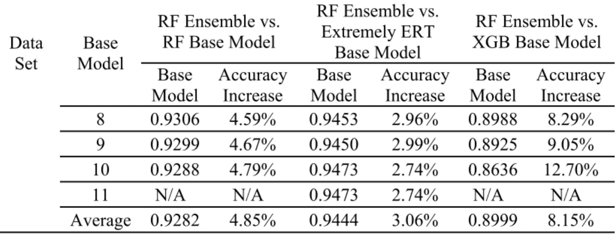
24.RF Ensemble in Experiment Two Compared with Base Models 70
25.Experiment Two Compared to Benchmarks and Experiment One 72
26.Ensemble Comparison in Experiment Two 73
27.MV Ensemble in Experiment Three Compared with Base Models 75
28.XGB Ensemble in Experiment Three Compared with Base Models 77
29.RF Ensemble in Experiment Three Compared with Base Models 79
30.LR Ensemble in Experiment Three Compared with Base Models 81
31.Experiment Three Compared to Benchmarks, Experiment One and Two 84
32.Ensemble Comparison in Experiment Three 85
33.XGB Ensemble in Experiment Four Compared with Base Models 88
34.RF Ensemble in Experiment Four Compared with Base Models 90
35.Ensemble Comparison in Experiment Four 92
36.Ensemble Accuracy of Experiment One, Two, Three, and Four 93
List of Figures
Figures
1. Ensemble all Base Models 34
2. Ensemble all Base Models and MCA Factor Scores 36
3. Ensemble with Model Selection 38
4. Ensemble with Factor Scores and Model Selection 42 5. Classification Accuracy of Random Forest Base Model 50
6. Classification Accuracy of Extremely Randomized Trees Base Model 51
Chapter 1
Introduction
Background
An ensemble approach integrates the output of a group of machine learning algorithms. The purpose of an ensemble approach is to achieve an improved classification accuracy that outperforms the individual learning algorithms which are often called base models. It has been shown that ensemble-based learning algorithms improve the predictive accuracy in many applications (Banfield, Hall, Bowyer, & Kegelmeyer, 2007; Leblanc & Tibshirani, 1996; Rodrigues, Kuncheva, & Alonso, 2006). Combining multiple learning algorithms has been found to be effective for various problems (Breiman, 2001; Zhang et al., 2011; Zhu, Beling, & Overstreet, 2002).
The initial step in an ensemble approach is creating various base models (Dietterich, 2001). The individual base models should be diverse enough in the sense that they have minimum errors in common. Base models can be generated 1) by different learning methods, 2) by using sub-samples of training data set, or/and 3) by using subsets of attributes or input features. Base models are generated by applying those three methods individually or together. Researchers in statistics and machine learning focus on constructing ensembles in which multiple base classifiers are
generated by perturbing or splitting the training data set. The training subsets are random samples with replacement or without replacement from the original training data. Several well-known ensemble-based learning algorithms, such as bagging, boosting, and random forest, have been widely accepted and applied for prediction tasks (Breiman, 1996 & 2001; Freund & Shapire, 1996). They have been shown to have consistently better performance than non-ensemble-based models.
The random forest (RF), extremely randomized trees (ERT), and extreme gradient boosting (XGB) models were applied in this dissertation to generate base models due to their high predictive accuracy (Brieman, 2001; Caruana & Niculescu, 2006; Geurts, Ernst, & Wehenkel, 2006; Friedman, 2001). They are all tree-based and ensemble-based machine learning algorithms. The RF model creates a large number of trees as base models by randomly selecting a subset of attributes in each splitting on randomly selected subsets of the training data (Brieman, 2001). Extremely randomized trees is a model similar to random forest. However, extremely randomized trees builds base classifiers on the whole training data by applying random selection on not only attributes but also the cut-point choice when splitting a tree node (Geurts, Ernst, & Wehenkel, 2006). The gradient boosting algorithm is an ensemble method in which the final classifier is combined by weak classifiers step by step (Friedman, 2001). In gradient boosting, a differentiable loss function is used to calculate the adjustments to the consecutive success learner in an iterative learning sequence. It assigns higher weights to misclassified observations when creating the subsequent tree. XGB is a scalable implementation of gradient boosting which is a very time efficient algorithm (Friedman, 2001; Friedman, Hastie, & Tibshirani 2000). By considering both training
loss and regularization, XGB can quickly reach the optimal decision and control overfitting at the same time.
Most commonly, all base models are ensembled together for the final output. However, researchers showed that combining a subset of base models with desirable characteristics worked better than combining all models (Ruta & Gabrys, 2005; Zhu, 2010). Selecting only a subset of base models might also contribute to both the accuracy of the final decision and the computing efficiency (Tsoumakas, Partalas, & Vlahavas, 2008). Jurek, Bi, Wu, and Nugent (2013) categorized base model selection techniques into static selection and dynamic selection. In static selection, the same subset of base models is used for both training and testing data sets (Zhu, 2010). While in dynamic selection, a subgroup of base models that locally perform better are chosen to make the decision (Cevikalp & Polikar, 2008). Base models can be selected based on either accuracy or diversity or both of these criteria (Jurek, Bi, Wu, & Nugent, 2003; Hu, 2001). Since the ensemble-based models, RF, ERT, and XGBoost as base models usually achieve good classification accuracy, this research focuses on applying correlation analysis and backward selection on the output of base models to identify an optimal subset of diverse base models, and multiple correspondence analysis (MCA) to capture the features of outputs of base models, thus to achieve more accurate predictions (Abdelazeem, 2008; Ruta and Gabrys, 2005).
After base models are selected, how to combine base models is the question to be addressed next. Researchers must consider and decide the kind of information to be integrated and the combining method to be applied. Generally, an ensemble approach integrates all or selected outputs of base models. The format of outputs from base
models varies, which can either be class label or probability. The combining technique can be majority voting, which is very effective when applying with a group of properly selected base models, such as decision trees in a random forest model (Breiman, 2001). It can also use various machine learning algorithms to integrate the outputs of base classifiers. For example, a logistic regression model is used to combine outputs of base models in stacking (Wolpert, 1992). Stacking, which is also called Stacked Generalization, has proven to be one of the most effective ensemble methods that improves the accuracy of the final decision of both classification and regression problems (Dzeroski & Zenko, 2004; Seewald, 2002; Jurek, Bi, Wu, & Nugent, 2001).
In this research, we chose random forest, extremely randomized trees, and extreme gradient boosting to construct base classifiers, applied model selection techniques, and integrated classifiers using various machine learning algorithms (random forest, logistic regression, and extreme gradient boosting). We systematically investigated the decision accuracy of the base models RF, ERT and XGB; how model selection techniques impacted the final ensemble result; the relationship between model combination techniques and the final ensemble results; and whether there existed a better ensemble approach.
Problem Statement
Improving predictive accuracy of machine learning algorithms is an ongoing research challenge. Numerous studies have shown that ensemble techniques increase the predictive accuracy when compared with non-ensemble-based classifiers for both classification and regression problem (Breiman, 1996; Dietterich, 2000; Leblanc and Tibshirani, 1996; Zhu, 2010). The majority of the related studies focused on integrating
weak classifiers, such as decision trees that were generated by perturbing the training data set (Breiman, 2000; Zhu, 2010). Researchers also demonstrated that picking several best models worked better than combining all models under some circumstances (Kotsiantis, 2011; Russell & Adam, 1987). The best models can be either those with various local predictive powers or those with the best predictive accuracy. Ensemble classifiers are particularly effective when the constituent base models are diverse in terms of their prediction accuracy in different regions of the feature space. The investigation of how to combine these ensemble-based models is a major research topic in the field of machine learning (Kotsiantis, 2011). In this dissertation, we studied methods for combining ensemble models by treating them as base models. Three tree-based ensemble methods – random forest, extremely randomized trees, and extreme gradient boosting model – were used to generate a set of base models (Brieman, 2001; Geurts, Ernst, & Wehenkel, 2006; Friedman, 2001). Outputs from classifiers generated by these methods were then combined to create an ensemble classifier to provide the final prediction. We systematically investigated methods for (1) selecting a set of diverse base models, and (2) combining the selected base models. The selection and combination methods were evaluated using public domain data sets which have been extensively used for benchmarking classification models.
Dissertation Goal
The goal of this dissertation is to develop a strategy for combining ensemble classifiers that results in higher classification accuracy than the constituent ensemble models. We investigated ensemble approaches which used random forest, extremely
Performances of base models were evaluated and compared. Correlation of outputs of base models were examined using Cramer’s V correlation analysis. Various base model selection techniques based on correlation or accuracy of base models were applied and compared. Different model combination techniques, majority voting if applicable, logistic regression, extreme gradient boosting, and random forest, were applied to all or optimal subsets of base classifiers. The performance of final ensemble outputs was evaluated.
Research Questions
1. Will specific ensemble approaches of ensemble-based models increase the predictive accuracy compared with extant single ensemble models?
2. Are random forest, extremely randomized trees, and extreme gradient boosting good candidates as base classifiers?
3. Will various model selection techniques make a difference in the predictive accuracy of the overall ensemble approach?
4. How will various model combination techniques affect the predictive accuracy of the ensemble approach?
Chapter 2
Review of the Literature
Overview
An ensemble approach starts from creating various base classifiers, selecting base classifiers, and ends in combining base classifiers. Various investigations have demonstrated that ensemble approaches of different classifiers improve the accuracy of the final classifier (Parvin & Alizadeh, 2011). Researchers evaluate learning algorithms by investigating the variance and bias (Kohavi & Wolpert, 1996). Variance measures the difference of prediction of a learning algorithm on different data sets. Bias measures the average error of a classifier trained with different training data sets. A single classifier usually has large bias and little variance when compared with a group of integrated classifiers (Webb & Conilione, 2003). It has been demonstrated that ensemble approaches usually reduce either variance or bias or both (Bauer & Kohavi, 1999).
The decision tree learning algorithm is a flowchart-like model that is widely used by researchers in information systems and machine learning. A decision tree model usually shows high variance in both choosing attributes and splitting nodes (Breiman, Friedman, Olshen, & Stone, 1984). It has been experimentally shown that cut-point variance of a decision tree model is extremely high for both small and large
data sets (Wehenkel, 1997; Geurts, 2000). The cut-point variance rephrases part of the error rate of the learning process. Because of the high variance, the decision tree is considered an unstable classifier. However, it works very well as the base classifier in ensemble approaches (Brieman, 2002). Several well-known ensemble approaches, such as boosting, random forest, and extremely randomized trees which incorporate a decision tree algorithm as the base models, are very successful in generating higher predictive accuracy (Breiman, 2002; Freund & Shapire, 1996). The idea behind these ensemble approaches is to reduce the variance of the learning algorithm without increasing the bias too much. These ensemble algorithms bring randomization into generating the same type of base classifiers (decision trees) on randomized training data sets. They generally are very competitive in producing better predictive accuracy than other non-ensemble-based machine learning algorithms (Dietterich, 2000).
It has been demonstrated that an ensemble model might avoid the mistake of choosing a wrong single model by statistically combining the output of base models, avoiding getting stuck in local optima computationally, and increasing the searching space for the true hypothesis (Dietterich, 2000). To avoid getting stuck in local optima and to increase the search space, diverse learning algorithms were often considered by researchers to include in the pool of base models (Kuncheva & Whitaker, 2003). Studies have demonstrated that the diversity of learning algorithms improves the accuracy of an ensemble approach (Dietterich, 2000). Diversity can be measured in various ways. A major measurement is to test the correlation of the decision output of each base model. The group of less correlated models tends to provide higher predictive accuracy (Hu, 2001). A different technique to evaluate the diversity of base models is
Q statistics test (Kuncheva & Whitaker, 2003). Clustering the outputs of base models and then adding clusters as additional attributes to the training dataset, and random selection of attributes or instances are proven techniques to increase the diversity of base models (Bryll, Gutierrez-Osuna, & Quek, 2003; Gan & Xiao, 2009). Among the stated methods, creating base models by randomly selecting either attributes or instances or both has been widely applied and has achieved tremendous success (Brieman, 2001).
Ensemble Models
Bagging
Brieman first proposed the idea of bagging which trained diverse individual base models by randomly selecting instances with replacement as training subsets (Breiman, 1996). It incorporates the idea of random selection which works by randomly selecting subsets of the training data set, manipulating the distribution of training data, or randomly selecting attributes (Breiman, 1996 & 2001; Freund & Shapire, 1996). Bagging is designed to reduce the variance of misclassification probability. Since base models can be trained independently, bagging can be very time-efficient. However, because of its strategy to create training data sets, bagging tends to improve the predictive accuracy by utilizing unstable classifiers, such as decision trees or artificial neural networks (Dietterich, 2000; Maclin, 1997). It has been shown that bagging is not able to improve the performance when using stable base models, such as linear regression (Skurichina, & Duin, 1998). Breiman (1996) explained that unstable models could be very diverse because they were sensitive to small changes of training data.
The diversity of base models is the key advantage of the bagging method to increase the final performance. However, at the same time, diversity also implies the unstable prediction of the randomly created base models. In order to obtain the same accuracy as an original decision tree, Machova and Barcak (2006) reported that the minimum number of base models in bagging should be twenty. Studies also reveal that bagging works more efficiently for small data sets (Skurichina, Kuncheva, & Duin, 2002).
Random Forest
Brieman (2001) proposed another ensemble approach, Random Forest, based on the idea of expanding diversity of base models by partitioning the attribute space. Random forest usually pools a lot of decision trees as base classifiers. It creates random training data sets for each individual decision tree by bootstrapping from the original training data set. It chooses the optimal attributes from a randomly selected subset of attributes at each split when growing a decision tree.
Random forest is an expanded version of bagging. The random subsets of instances don’t have the same number of instances as the original training set. Generally, each subset has two thirds of the instances of the whole training data. At each split, an optimal attribute is chosen from around two thirds of the randomly selected attributes. Random forest not only adopts the advantages of bagging, such as more diversity of base classifiers and computational efficiency, but also overcomes some weaknesses of bagging, such as dealing with both small and large data very efficiently. Additionally, it is also designed to deal with the overfitting issue. Random forest is a very competitive and successful ensemble model and has been applied to
different research fields (Chi, Yeh, & Lai, 2011; Diaz-Uriarte & Alvarez de Andres, 2006).
Extremely Randomized Trees
Extremely Randomized Trees is another ensemble-based model. It is also called Extra Trees. It takes randomization even further when compared with random forest (Geurts et al., 2006). It randomizes not only the selection of instances and attributes, but also the selection of the cut point of splitting when growing individual base trees. The structures of total random trees are independent of the output of learning data. It is also extremely computationally efficient due to the extreme randomization.
The extremely randomized trees model works by decreasing variance while increasing bias at the same time. However, referenced to the standard decision tree model, if the randomization degree is optimal leveled, the variance can be extremely diminished and the bias increases only a little bit. The extremely randomized trees model has been demonstrated to be the top choice in many applications, such as high dimensional problems, mass-spectrometry datasets, and time series classification problems (Geurts & Wehenkel, 2005; Geurts, Fillet, De Seny, Meuwis, Mervilles, & Wehenkel, 2005b; Maree, Geurts, Piater, & Wehenkel, 2004). It has a very strong competitive predictive power, especially for classification problem, when compared with random forest and other ensemble approaches (Geurts et al., 2006).
Boosting
Another well-known ensemble technique, Boosting, was proposed by Freund and Schapire in 1996. It utilizes the random selection idea and manipulates the
distribution of training data by creating subsequent base models based on the predictive accuracy of previous base models. It is an iterative procedure that adds base classifiers one by one. Weights of one base model are calculated based on its predictive accuracy and are then applied when integrated with other base models. Weights of instance are also calculated by the current base model, and then are used to train the next base model. In this way, base models are regulated and the weighted predictions of the base models are combined to make the final decision. Boosting has been shown to reduce variance and bias (Rodriguez & Maudes, 2008). Good candidates for base models are decision trees or neural networks (Rodriguez & Maudes, 2008; Schwenk & Bengio, 2000).
Ada boosting is the benchmark model in boosting (Schapire, 1999). A number of studies have been explored to expand the techniques of Ada boosting to improve the accuracy and efficiency (Schapire, Freund, Bartlett, & LeeWS, 1998). Gradient boosting is one of its expansion forms and has earned a good reputation for its excellent performance in both accuracy and efficiency when compared with Ada boosting (Friedman, 2001). It utilizes a loss function to manipulate the adjustment that is applied to the subsequent base model. The training loss function measures how the model fits on training data. The gradient boosting model not only measures the model fit but also regulates the model complexity using a regularization function. Optimizing loss function tends to cause over-fitting. On the contrary, optimizing regularization function produces smaller variance for prediction. Balancing loss and regularization functions properly can produce optimal predictive performance and control the over-fitting issue (Johnson & Zhang, 2014).
Extreme gradient boosting is an algorithm created under the framework of gradient boosting (Chen, 2015). It utilizes generalized linear model and gradient boosted decision trees. Randomly sub-setting the instances and attributes techniques are applied in the extreme gradient boosting algorithm. It is very efficient in handling sparse matrices and producing accurate predictions.
Model Selection
Most ensemble approaches integrate all base models to make the final prediction. However, it has been shown that effective selection of a group of optimal base models based on diversity and accuracy can improve the final ensemble performance (Zeng, Chao, & Wong, 2010).
Abdelazeem (2008) proposed forward search or backward search methods to select an optimal set of base models based on majority voting error of the ensemble model. The forward search starts from the most accurate base model and adds other base models one by one until there is no improvement of predictive accuracy. The backward search starts from combining all of the base models, and then excludes base models one by one until the decrease of predictive accuracy is not acceptable.
Genetic algorithm (GA) has been applied in searching the best subset of base models when considering the accuracy of both base and final ensemble models (Kittler & Roli, 2001). Both diversity and accuracy are evaluated when applying the GA approach (Löfström, Johansson, & Bostrom, 2008). It is revealed that considering the accuracy of both the base and ensemble models is the most efficient approach for the GA approach of model selection.
Ruta and Gabrys (2005) selected the optimal subset of base models by evaluating various diversities of the models. In their approaches, diversities were presented by correlation coefficient, product moment correlation, Q statistics, disagreement measure, double-fault, entropy, and measure of difficulties. In addition to diversities, accuracies such as minimum individual error, mean error, and majority voting error were also considered. Various search methods, such as forward and backward search, random search, and GA search were explored. The experiment result showed that using majority voting error as the search criterion was the best way for model selection.
Model Integration
The last step in the ensemble approach is integrating the outputs of base models to make the final decision of regression or classification problems. The combination methods can be simple averaging, majority voting, or using functions or machine learning algorithms to combine base models (Brieman, 2001; Wolpert, 1992).
Majority voting is a simple but effective method, in which the final decision of an instance is voted by all base models. The case receiving the most votes is the final decision. An expanded version of majority voting is adding weights to base models where the weights are scaled by the accuracy or entropy of the base models. This weighting method has been expanded further by applying genetic algorithms (GA) to optimize the final result (Dimililer, Varoglu, & Altincay, 2007).
Stacked generalization is also an alternative way to combine multiple models (Wolpert, 1992). It works by reducing biases of learning algorithms with respect to a specific training data set. In stacked generalization, the outputs of base models for the
validating data set compose the training data for a meta-model. Then, a meta-learner is generated by a machine learning algorithm to combine the outputs of base models. Effective machine learning algorithm for the meta-learner can be multi-response linear regression and multi-response model tree (Dzeroski & Zenko, 2004; Seewald, 2002; Ting & Witten, 1999). Majority voting is not preferred in stacked generalization because it usually does not work on comparable or similar outputs of base models (Ting & Witten, 1999). However, the multilayer perceptron has been demonstrated to be an effective algorithm to combine the outputs of base models (Zhu, 2010). Logistic regression has also proved to be successful in combining outputs of base models in stacking (Wolpert, 1992).
Chapter 3
Methodology
Overview of Research Methodology
In this research, we explored an ensemble approach in which tree-based ensemble learning algorithms are used as base models. The primary goal is to study if an ensemble approach of ensemble-based models would further improve predictive accuracy. The secondary goal is investigating effective ways for selecting base models and various combination strategies. The overall ensemble procedure includes four
major steps:
1. generating base models
2. calculating factor scores of multiple correspondence analysis 3. choosing optimal subsets of base models, and
4. integrating base models Generating base models
Ten random forest, eleven extremely randomized trees (extra trees), and ten extreme gradient boosting models were generated to work as base models to ensemble. All base models are tree-based ensemble models (Brieman, 2001; Geurts et al., 2006; Freund & Schapire, 1996). They have proved to be relatively better models which
provide higher predictive accuracy. They all apply a randomization scheme to expand the diversity of base models in order to achieve better ensemble result.
Random Forests: The steps of building a random forest are listed as follows (Breiman, 2001).
1. To create a forest with trees, subsets of data are sampled with instances randomly with replacement. Each subset grows one individual tree. Usually, the size of a subset is about two thirds of the size of the training set.
2. When building a single tree, at each splitting of node, predictor variables are chosen randomly from all available variables. Each predictor is evaluated by a selected objective function. The one which provides the best splitting is used to do a binary split on that node. The same procedure is applied to all remaining nodes. The value of can range from 1 to the total number of predictor variables. Most researchers set to be the square root of the total number of predictor variables (Brieman, 2001).
3. trees are created by repeating step 1 & 2 to construct a forest. When a new set of instances is input into the forest, one by one, each instance goes through every tree in the forest. The predictive result is the majority voting of the trees for a classification problem.
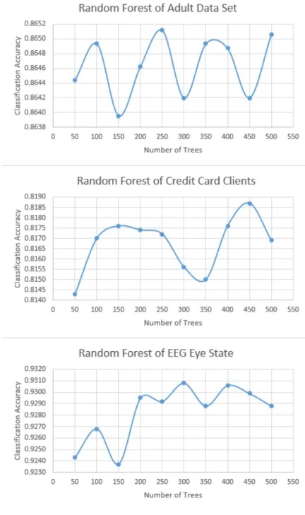
4. Ten random forests were built on training data sets in this research. Seeds were randomly set up to ensure a repeatable predictive result for each forest. The number of individual trees in the forest ranged from 50 to 500. Because of the randomization strategy of sub-setting the instances and attributes and setting up different seeds and number of subtrees when building a random forest, these ten
forests had different structures and provided different predictions on the testing data set. Table 1 lists the number of trees of each base model.
Table 1
Number of Trees in Random Forest Base Model Radom Forest Number of Trees
1 50 2 100 3 150 4 200 5 250 6 300 7 350 8 400 9 450 10 500
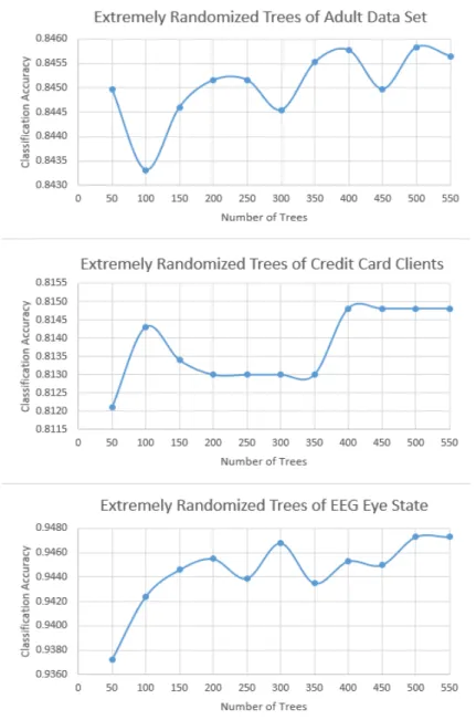
Extremely Randomized Trees: The procedure of building extremely randomized trees, also called extra trees, is listed as follows (Geurts et al., 2006). 1. decision trees are built without pruning from all training sample.
2. At each random splitting of a node, predictor variables, , … , , among all
non-constant candidate predictors are chosen without replacement and evaluated to split the node. splits, , … , , one split per predictor, are generated from predictors. A split ∗is selected if its score of evaluation is the most preferred one
among all of the splits. The same procedure is applied to each node.
3. Numerical predictors and categorical predictors follow different rules of splitting. For a categorical predictor , is used to denote its domain or the set of all possible values. is a subset of in which every value a appears in the training set S.
Then, a proper nonempty subset of and a subset of A\ is randomly drawn. The split that meets [a∈ ∪ ] is returned to compare with other splits.
For a numerical predictor a, its maximal and minimal value in S, ,
are calculated. A cutout point is uniformly drawn in [ , ]. The split that
meets [ ] is returned.
4. The trees created by repeating step 2 & 3 are used to construct an extra trees model. When a new set of instances is input into the forest, one by one, each instance goes through all of the trees in the extra trees model. The result is the majority voting of the trees for a classification problem.
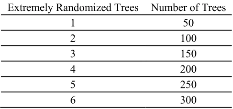
5. Eleven extra trees models were built in this research. Seeds were randomly set up to ensure repeatable predictive result for each extra tree model. The number of individual trees in an extra trees model ranged from 50 to 550. Because of the randomization of sub-setting the instances and attributes, and setting up different seeds and number of subtrees when building an extra tree, these eleven extra trees had different structures and provided different predictions on the testing data set. Table 2 lists the number of trees in each model.
Table 2
Number of Trees in Extremely Randomized Trees Base Model Extremely Randomized Trees Number of Trees
1 50 2 100 3 150 4 200 5 250 6 300
Extremely Randomized Trees Number of Trees 7 350 8 400 9 450 10 500 11 550
Extreme Gradient Boosting: Extreme gradient boosting model (XGB) is a tree-based ensemble model created under the gradient boosting framework proposed by Friedman (2001). Efficient linear solver and tree learning algorithm are implemented in XGB (Chen & He, 2015). The approach of constructing an XGB model is listed as follows (Chen & He, 2015).
1. XGB model is a summation of a collection of weak trees. It is defined as
∑ , where is the prediction of a decision tree.
2. Let denote the feature vector for the i-th data point, the prediction with all the
decision trees can be expressed as ∑ . In each iteration step, one
tree is added to the collection, at the t-th step, the prediction is defined as
∑ .
3. When training the model, a loss function is chosen and optimized based on different types of task. For a binary classification problem, LogLoss is used as the loss function.
L 1 log 1 log 1
where is the real value of prediction on feature vector , is the probability on feature vector , and is the number of instances in the training data set. For a
multi-classification problem, mlogloss is used as the loss function which is defined as below, where is the number of categories of target feature.
L 1 , log ,
4. When optimizing the loss function, XGB also implements a regularization term Ω to control the complexity in order to prevent overfitting.
Ω Ƭ 1
2
is the number of leaves. Instead of , which is the score on the j-th leaf that is used for better controlling the complexity. λ and both tune the complexity. 5. The objective function of XGB is defined as the combination of loss function and
regularization. Loss function controls the predictive power and regularization controls the simplicity.
Ω
6. Gradient descent is applied to optimize the objective function , . It is an
iterative technique that calculates , at each iteration. is improved along the direction of the gradient to minimize the objective.
7. For an iterative algorithm, the objective function at each step can be rewritten as
, Ω , Ω
The first and second order gradient are calculated to
improve the performance. The Taylor approximation of the objective function is derived as follows since there might be no derivative for every objective function.
≅ , 1
2 Ω
Where L , and L ,
Removing the constant terms since they don’t affect the optimization, the objective function at the t-th step is derived below. The goal is to find a to optimize .
1
2 Ω
8. Finding a tree in each step to improve the prediction along the gradient is critical in XGB. For a decision tree, internal node defines the data point flowing direction. Each leaf is assigned a weight, which is the prediction. Mathematically, a tree can
be defined as , where is a directing function that assigns every
data point to the -th leaf. is the corresponding score on the -th leaf.
An index set is also defined as | . It contains the indices of data
points that are assigned to the j-th leaf. Rewriting the objectives in terms of leaves, the objective function becomes
1 2 Ƭ 1 2 1 2 ∈ ∈
The objective function in this form would be optimized by . The best
that optimizes the objective function is ∑∑∈
∈ , and the corresponding
1 2
∑∈ ∑∈
9. When building a tree, to find the best splitting point that can optimize the objective function, the best splitting point of each attribute is identified first, then the best attribute is picked out based on the objective function. Since is the set of indices of data points that assigned to a node, and are the sets of indices of data points that assigned to two new leaves. The gain of splitting is calculated based on optimal objective function. The split that achieves the most gain is the best one.
1 2 ∑∈ ∑∈ ∑∈ ∑∈ ∑∈ ∑∈
r is the complexity cost by introducing additional leaf. The tree is built to the maximum depth in this way, and is pruned by taking out the nodes with negative gains in a bottom-up order.
10.When building an individual tree, a subset of instances is sampled. At each split, a subset of attributes is also randomly selected. A XGB model can be created by following steps in 1 through 9.
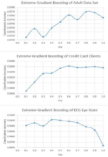
11.We constructed ten XGB models as base models in this research. Setting up seed was tried randomly to ensure a repeatable predictive result for each XGBoost model. However, it didn’t work and couldn’t provide s repeatable prediction. Parameter “eta” in the R XGBoost package was adjusted from 0.1 to 1 to control the gradient speed. They are listed in table 3 for reference. Parameter “nround” was optimally chosen by a 10-fold cross validation method based on parameter “eta”. As a result, the number of individual trees in each XGB model was different,
therefore these ten XGB models had different structures and provided a different prediction on testing data set.
Table 3
Parameter Eta in Extreme Gradient Boosting Base Model
Extreme Gradient Boosting Eta
1 0.1 2 0.2 3 0.3 4 0.4 5 0.5 6 0.6 7 0.7 8 0.8 9 0.9 10 1.0
Calculating factor scores of multiple correspondence analysis
Multiple correspondence analysis (MCA) was applied to the outputs of the base models (Le Roux & Rouanet, 2004; Greenacre & Blasius, 2006). Factor scores of individual output instances were produced (Abdi & Valentin, 2007). They were added as new attributes to ensemble with the outputs of base models in the final ensemble step (Zhang & Zhang, 2009). MCA is a statistical procedure that applied to categorical variables, which represents data in a low-dimensional Euclidean space. In our study, conducting MCA converted the outputs of base models into a set of factor scores.
Since the dissertation is focused on classification problems, we kept the outputs of base models in categorical format. Each output must be reconstructed into
another set of binary variables with only 0 and 1 as their values. For example, for a binary output Salary with two categories “more than $50,000” and “not more than $50,000”, two new variables “more than $50,000” and “not more than $50,000” are created to replace the categorical output. For a person with salary more than $50,000, the corresponding value of the new variable “more than $50,000” is 1, and “not more than $50,000” is 0. In this way, each categorical output with levels is replaced by new binary variables. With B outputs in total, new binary variables were created and set into the MCA approach. For observations, an indicator matrix with columns and rows was formed.
A correspondence analysis (CA) was then performed on the indicator matrix. Letting denote the sum of elements of indicator matrix, the probability matrix is .The vector of row sums of is denoted as . The vector of column sums of is denoted as . The following singular value decomposition is performed.
∆
where diag , diag , ∆ is the diagonal matrix of the singular values
which is calculated from ∆ , the matrix of eigenvalues. Row and column factor scores, F and G, are calculated as follows:
∆ ∆
These factors scores are considered as inheriting the maximum possible variance from . Although MCA produces row and column factor scores, in our approach, only the
column factor scores were ensembled with the outputs of base models in the last ensemble step.
Choosing optimal subsets of base models
Choosing optimal subsets of base models is the third step in the whole procedure. Various model selection techniques could be applied to choose optimal subsets of base models to ensemble. The following two methods were used in this research for model selection.
Cramér's V correlation analysis: Cramér's V correlation between outputs of base models on testing data is calculated. Then, a criterion or a cutout point of correlation coefficient is picked, and the most uncorrelated models are chosen as the group of optimal base models (Cramér, 1946).
For outputs of base models { , , … , }, Cramér's V correlation
coefficient measures the pairwise association between them. The association is based on Pearson’s chi-square statistics. ranges from 1 to 31 since thirty-one base models were generated in total. Cramér's V correlation coefficient is calculated based on the
following formula. For two outputs of base model, and , , ∀ 1, … , , and
∀ 1, … , , a contingency table is created in table 4, is the number of classes of the output variable.
Table 4
Contingency Table of Cramér's V Correlation Category of Output 1 , , 2 , , . . . . . . . . . k , ,
, is the number of class observed in the output . , is the number of
class observed in the output . The chi-squared statistic is calculated as below
, ,
, Cramér's V correlation coefficient is
⁄ 1
φ 1
where is the grand total of observations, φ is the phi coefficient.
Cramér's V correlation coefficient ranges from 0 to 1. A value close to 0 indicates less correlation between two outputs. Since the base models are expected to be accurate, which leads their pairwise correlation coefficients closer to 1. The cutout point value of its absolute value varies based on different data sets. We chose base model pairs whose correlation coefficient was closer to 0 as members of the optimal subset.
Backward selection: A backward selection of base models was applied in the research based on Akaike Information Criterion (AIC) value provided by the logistic regression ensemble models. AIC was originally introduced to measure the relative
quality of models on the same set of data set (Hocking, 1976; Bozdogan, 1987). It is defined as follows,
2 2ln )
where is the number of estimated parameters in a model, is the maximum value of the likelihood function of logistic regression model. In this research, the data set contains the output of base models . For outputs of base models { , , … , }, this approach starts from ensemble all of the outputs of base models by logistic regression model below.
1
Where ⋯ , and , , … , are the fitted coefficients
of logistic regression.
In this research, the backward selection method excluded one base model in each round to reach the goal of not significantly losing predictive power with the smallest number of base models. If denotes the number of base models, in each round, AICs of number of logistic regressions were compared. Here, each logistic
regression was created by combining 1 number of base models by omitting one
base model. Each base model was excluded once in a logistic regression. Thus, the resulted AIC value of logistic regression presented the effect of each base model to the predictive power. One base model was chosen to exclude in the next round if omitting it resulted in the smallest AIC value. The backward selection stopped if excluding any one of the remaining base models would not make the AIC significantly lower than that in the previous round. Here, the chi-square statistic was applied to determine the significance of AIC decreasing at 0.05 level in the study.
Integrating base models
In the last step of the ensemble approach, majority voting, random forest, extremely gradient boosting, and logistic regression models were applied to integrate the outputs of base models with 1) all base models, 2) all base models and factor scores of multiple correspondence analysis, 3) the optimal subsets of base models chosen by
Cramér's V and backward model selection, or 4) factor scores and the optimal subsets of base model chosen by Cramér's V correlation and backward model selection. The misclassification rate was used to compare all of the ensemble results.
Software and Code
Experiments were conducted in RStudio of R version 3.3.1 (R Core Team, 2016). RStudio is an integrated development environment (IDE) for R. Compared to R, RStudio is designed to be more user-friendly. Researchers can code, edit, and run R codes in RStudio. The open-sourced RStudio is available to download for free and is used in this research. The RStudio for windows desktop was chosen and downloaded from the following website, https://www.rstudio.com, by selecting platform x86_64-w64-mingw32/x64 (64-bit). A screen shot of RStudio interface can be found in Appendix A.
Since many researchers contribute their research results to the R community for free, the R community is the first or best place for a researcher to find solutions to classification problems. Random forest, extremely randomized trees (extra trees), and extreme gradient boosting model are all available in the R community, so R becomes an accessible option to conduct experiments in this dissertation. In addition to the
models mentioned above, multiple correspondence analysis and other well-known statistical analyses are all available in the R community. Data manipulation and calculation are also convenient to conduct in R. Due to the easy access to the R community and documentation and tutorial of R programming, R code was used in RStudio for all the experiments in this research.
In addition to basic R programming, research ideas are contributed to the R community and presented by researchers in R packages. The three types of models, random forest, extremely randomized trees, and extreme gradient boosting, are presented in three R packages, XGBoost, extraTrees, and randomForest. They have been widely used by many researchers in their research (Chen, 2014; Chen & He, 2015; Diaz-Uriarte, & Alvarez de Andres, 2006; Geurts et al., 2006). The manual of all R packages, related R code, and examples are saved in the Comprehensive R Archive Network (CRAN) and maintained regularly by the authors. CRAN can be accessed at https://cran.r-project.org/. Detailed information of R packages of random forest, extremely randomized trees, extreme gradient boosting, and logistic regression model are listed in table 5. The syntax of conducting models in R code can be found through the links provided in the reference list.
Table 5
R Packages of Models
Model R Package Reference
Extreme Gradient Boosting xgboost Chen , He , & Benesty, 2016
Extremely Randomized Trees extraTrees Simm, & Magrans de Abril, 2014
Random Forest randomForest Breiman, Cutler, Liaw, & Wiener, 2015
In addition to R packages which generate the above base models or ensemble models, multiple correspondence analysis and Cramér's V correlation analysis were also applied in the experiments in RStudio. The related R packages, ca and vcd, are listed in table 6.
Table 6
R Packages of Analysis
Analysis R Package Reference
Multiple Correspondence ca Greenacre, Nenadic, & Friendly, 2016
Cramér's V correlation vcd David, Achim, Kurt, Florian, &
Michael, 2016
Several other R packages, which supported models and analysis in the research, are listed in table 7. They were used for data manipulation and calculation, such as installing R packages, binarizing predictors, supporting extra tree package, and calculating variable importance when building a model, selecting base models, and integrating base models.
Table 7
Supportive R Packages
R Package Function Reference
caret Data manipulation Kuhn et al., 2016
DiagrammeR Plot variable importance Iannone, 2016
Ckmeans.1d.dp Plot variable importance Song & Wang, 2016
rJava Support Extra Tree package Urbanek, 2016
Data Sets
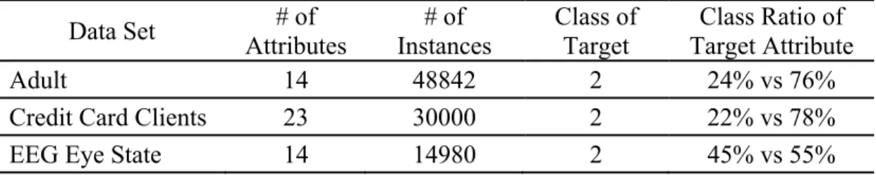
The research experiments were conducted on three UCI data sets that are public and free to download (Lichman, 2013; Blake & Merz, 1998). UCI is a repository of machine learning database. These data sets are real-world data and extensively used by researchers in many research studies (Ron, 1996; Yeh & Lien, 2009; Thuraisingham, Tran, Boord & Craig, 2007). These three data sets represent binary classification problems with different class ratios of the target attribute. They were used to test if the proposed ensemble approach achieved better classification accuracy on binary classification problems. The profiles of the three data sets are listed in table 8.
Table 8 Data Sets
Data Set Attributes # of Instances # of Class of Target Target Attribute Class Ratio of
Adult 14 48842 2 24% vs 76%
Credit Card Clients 23 30000 2 22% vs 78%
EEG Eye State 14 14980 2 45% vs 55%
Note: # means count
The Adult data set is provided by UCI as two separate sets: training and testing data sets. The Credit Card Clients and EEG Eye State data sets were partitioned into training and testing data sets in a 70% vs. 30% ratio. Base models were built on training data sets. Prediction was provided by base models on testing data sets. The number of instances in training and testing data sets are listed in table 9 as follows.
Table 9
Training and Testing Data Sets
Data Set Number of Instances in
Training Set
Number of Instances in Testing Set
Adult 32561 16281
Credit Card Clients 21000 9000
EEG Eye State 10486 4494
Experiment Design
There are four experiment designs. They were designed to explore how model selection, MCA factor scores, and ensemble method affected the classification accuracy. They were also designed to identify ensemble strategies to improve the ensemble performance. Detailed designs and what research questions were answered are presented and explained below.
1. Ensemble all base models
2. Ensemble all base models and MCA factor scores
3. Ensemble with backward or Cramér's V model selection
4. Ensemble with MCA factor scores and backward or Cramér's V model selection
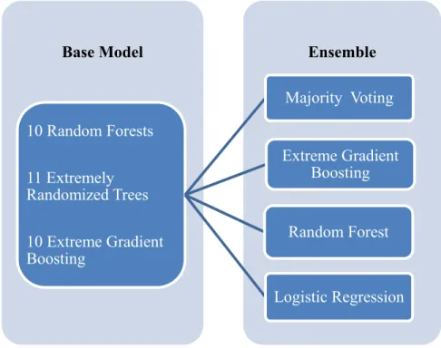
Ensemble all Base Models
This experiment was performed in the following steps. Ten base models of random forest (RF), eleven extremely randomized trees (ERT), and ten extreme gradient boosting (XGB) models were first generated. Then, majority voting, random forest, and extreme gradient boosting model were applied to ensemble all of those
thirty-one base models. The only reason for creating eleven extremely randomized trees is to avoid even voting of the binary classification of target in the majority voting ensemble. There is also no specific reason for choosing extremely randomized trees as the thirty-first base model.
The average accuracy of ten random forest base models was considered as the benchmark in our research because of its well-known reputation of good performance. The accuracy of ensemble results was compared with that of each base model and the benchmark to find out whether the four ensemble methods helped to increase the accuracy. The accuracy of ensemble results was also compared with each other. The best ensemble method among random forest, extreme gradient boosting, logistic regression and majority voting was identified when integrating the thirty-one base models.
Figure 1. Ensemble all Base Models
Ensemble Base Model 10 Random Forests 11 Extremely Randomized Trees 10 Extreme Gradient Boosting Majority Voting Random Forest Extreme Gradient Boosting Logistic Regression
The experiment answered the following research questions.
1. Will the four ensemble approaches of ensemble-based models increase the predictive accuracy when compared with the benchmark or the individual ensemble models?
2. As base classifiers, are random forest, extremely randomized trees, and extreme gradient boosting models good candidates to be ensembled?
3. How will various model combinations (majority voting, random forest, extreme gradient boosting, and logistic regression) affect the predictive accuracy of the ensemble approach?
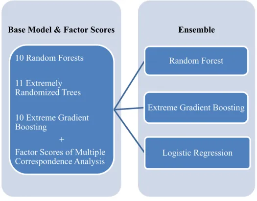
Ensemble all Base Models and MCA Factor Scores
In addition to the experiment that integrated all base models, the experiment in this section was performed by adding factor scores of multiple correspondence analysis. Multiple correspondence analysis was applied to the predictions of thirty-one base models to generate MCA factor scores. MCA factor scores were considered to represent the maximum variance of the thirty-one base models. Because of the different nature of individual data sets, a different number of sets of factor scores were generated for the three data sets used in the experiment. The number ranged from 4 to 6. Random forest, extreme gradient boosting, and logistic regression model were applied to ensemble all the base models and the factor scores of multiple correspondence analysis. In this experiment, the base models are the same as those in the first experiment design. Majority voting is not applicable in the experiment because MCA factor scores were numerical but not categorical attribute for ensemble.
The performance of ensemble results was compared with those of each base model and the benchmark to determine whether the four ensemble methods increased the predictive accuracy. Compared with the experiment that only integrated base models, the factor scores of multiple correspondence analysis were added as predictors in the final ensemble to identify whether adding MCA factor scores increased the predictive accuracy.
Figure 2. Ensemble all Base Models and MCA Factor Scores
The three ensemble results were compared with each other. The one with the best performance among random forest, extreme gradient boosting, and logistic regression was determined when combining the thirty-one base models and MCA factor scores.
The experiment answered the following research questions.
Ensemble Base Model & Factor Scores
10 Random Forests 11 Extremely Randomized Trees 10 Extreme Gradient Boosting +
Factor Scores of Multiple Correspondence Analysis
Random Forest
Extreme Gradient Boosting
1. Will the three ensemble approaches of ensemble-based models increase the predictive accuracy when compared with the benchmark or the individual ensemble models?
2. As base classifiers, are random forest, extremely randomized trees, and extreme gradient boosting model good candidates to be ensembled with MCA factor scores?
3. Will the multiple correspondence analysis make a difference on the predictive accuracy of the overall ensemble approach?
4. How will various model combinations (random forest, extreme gradient boosting, and logistic regression) affect the predictive accuracy of the ensemble approach?
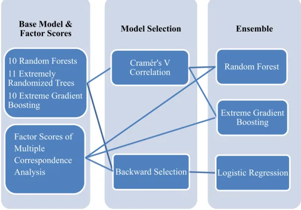
Ensemble with Cramér's V correlation or Backward Model Selection
Compared with the second experiment design, the model selection procedure was added in, but factor scores of multiple correspondence analysis was excluded from the experiment presented in this section. Two methods, Cramér's V correlation or Backward Model Selection, were applied in the model selection step. The whole procedure includes three steps: base model generation, model selection, and ensemble. The base models generated in the first step are the same as those in the previous experiment designs.
The first model selection method is derived from Cramér's V correlation analysis. In this method, Cramér's V correlation coefficient is calculated between each pair of base models. Paired base models with correlation coefficient lower than a
base models, base models which are less correlated with each other were kept. The final ensemble method was applied to the selected base models by majority voting, random forest, and extreme gradient boosting model. Since the threshold of Cramér's V correlation coefficient value was hard to determine, we didn’t use individual correlation coefficient as the cutout point to pick the least related base models. We evaluated the average value of Cramér’s V correlation coefficient between different types of base models to select two types of least correlated base models. The base models in those two types were selected and kept in the final ensemble procedure. The Cramér's V correlation coefficients of each paired base models on the three data sets are presented in Appendix C, D and E. It is shown that extreme gradient boosting and extremely randomized trees base models have the smallest average Cramér's V correlation coefficient for the three data sets. Therefore, all extreme gradient boosting and extremely randomized trees base models were selected as the optimal base models and combined in the final ensemble step.
Figure 3. Ensemble with Model Selection
Ensemble Model Selection Base Model 10 Random Forests 11 Extremely Randomized Trees 10 Extreme Gradient Boosting Cramér's V
Correlation Random Forest
Extreme Gradient Boosting Majority Voting
Backward Selection Logistic
Another model selection method is backward selection based on Akaike's information criterion (AIC) which is combined with logistic regression model. This model selection procedure starts from ensemble all base models. Then, base models are removed one by one in the ensemble step until the AIC value doesn’t decrease significantly at 0.05 level. In each round, the base model that contributed to the AIC the most is chosen and excluded in the next round.
The accuracy of ensemble results was compared with those of each base model and the benchmark to determine whether the four ensemble methods with model selection was able to increase the predictive accuracy. The best candidate base models chosen by different model selection methods were selected. Compared with the experiment design which integrated all base models without model selection, we added the model selection procedure in the experiment presented in this section. By comparing the performance of those two experiments, we were able to find out whether the model selection procedure can help to increase the predictive accuracy. Lower predictive accuracy might be observed because a smaller number of base models, which meant less information, were used in the final ensemble. Whether model selection helped on combining tree-based ensemble models was also learned by comparing the ensemble performance in experiment two.
The accuracy of ensemble results of the two model selection methods was compared to find out which one was the better model selection method. We also identified which combination of model selection method and final ensemble method worked the best together in increasing predictive accuracy.
1. Will the four ensemble approaches of ensemble-based models increase the predictive accuracy when compared with the benchmark or the individual ensemble models?
2. Are random forest, extremely randomized trees, and extreme gradient boosting good candidates as base classifiers when applying model selection in ensemble? 3. How will various model combinations (random forest, extreme gradient boosting, and logistic regression) affect the predictive accuracy of the ensemble approach?
4. Will the two types of model selections make a difference in the predictive accuracy of the overall ensemble approach?
Ensemble with MCA Factor Scores and Model Selections
In this experiment design, factor scores of multiple correspondence analysis were added into the experiment. The whole procedure involved three steps, base model and factor score creation, base model selection, and ensemble. In the first step, ten random forest, eleven extreme randomized trees, and ten extreme gradient boosting base models were created. They were the same base models as those in the previous three experiment designs. Then, multiple correspondence analysis was applied to the predictions of the base models to generate the factor scores of MCA. The factor scores of MCA were also the same as those in the second experiment design. MCA factor scores were then integrated together with the selected base models in the final model ensemble step by logistic regression, random forest, and extreme gradient boosting model. Since majority voting ensemble can only be applied to the outputs of base
models, but MCA factor scores were not outputs of base models, majority voting ensemble was not applicable in the experiment.
The two model selection methods, backward AIC selection and Cramér’s V correlation selection, were used in this experiment. The backward selection method started from combining all base models and MCA factor scores. Model selection and ensemble worked together to evaluate base models and MCA factor scores one by one, and then determine which base model or factor scores contributed the most AIC that provided by logistic regression ensemble in each round. The identified base model or factor scores would be excluded in the next round of evaluation. Only one base model or one factor score was eliminated in each round. The AIC value of logistic regression model in each round was compared with that in the previous round. If the AIC value didn’t decrease significantly at 0.05 level, the backward selection stopped. The experiment showed that the same group of base models was selected as in experiment three. Figure 4 shows the experiment structure of logistic regression ensemble with backward selection.
The accuracy of the ensemble result was compared with the accuracy of each base model and the benchmark.Whether integrating the backward model selection and factor scores increased the predictive accuracy was determined. Compared with the ensemble method without factor scores but with backward model selection, whether the method that integrated the factor scores with backward selection increased the predictive accuracy was learned.
Figure 4. Ensemble with Factor Scores and Model Selection
The second model selection method is applying Cramér's V correlation analysis to select the least correlated base models. Cramér's V correlation coefficient is calculated between each base model. Ideally, paired base models with a correlation coefficient lower than a threshold value are kept to ensemble with factor scores in the final ensemble step. However, the correlations between base models on different data sets vary, thus the threshold is not easy to determine. We decided to evaluate the average correlation coefficients of different types of base models. Two types of base models that had the lowest average correlation were chosen. Then all base models in these two types were combined in the final ensemble. The selection procedure and the selected base models are the same as those in experiment three. It was shown that extreme gradient boosting and extremely randomized trees base models had the
Ensemble Model Selection
Base Model & Factor Scores 10 Random Forests 11 Extremely Randomized Trees 10 Extreme Gradient Boosting Cramér's V
Correlation Random Forest
Extreme Gradient Boosting
Backward Selection Logistic Regression
Factor Scores of Multiple
Correspondence Analysis