Structural Analysis of Network Traffic Flows

(1)

Structural Analysis of Network Traffic Flows

Anukool Lakhina, Konstantina Papagiannaki, Mark Crovella,

Christophe Diot, Eric D. Kolaczyk, and Nina Taft

ABSTRACT

Network traffic arises from the superposition of Origin-Destination (OD) flows. Hence, a thorough understanding of OD flows is essen-tial for modeling network traffic, and for addressing a wide variety of problems including traffic engineering, traffic matrix estimation, capacity planning, forecasting and anomaly detection. However, to date, OD flows have not been closely studied, and there is very little known about their properties.

We present the first analysis of complete sets of OD flow time-series, taken from two different backbone networks (Abilene and Sprint-Europe). Using Principal Component Analysis (PCA), we find that the set of OD flows has small intrinsic dimension. In fact, even in a network with over a hundred OD flows, these flows can be accurately modeled in time using a small number (10 or less) of independent components or dimensions.

We also show how to use PCA to systematically decompose the structure of OD flow timeseries into three main constituents: com-mon periodic trends, short-lived bursts, and noise. We provide in-sight into how the various constitutents contribute to the overall structure of OD flows and explore the extent to which this decom-position varies over time.

A. Lakhina and M. Crovella are with the Depart-ment of Computer Science, Boston University; email:

fanukool,[email protected]. K. Papagiannaki

and C. Diot are with Intel Research, Cambridge, UK; email:

fdina.papagiannaki,[email protected].

E. D. Kolaczyk is with the Department of Mathe-matics and Statistics, Boston University; email:

[email protected]. N. Taft is with Intel Research,

Berkeley; email: [email protected]. This work was performed while M. Crovella was at Laboratoire d’Informatique de Paris 6 (LIP6), with support from Centre National de la Recherche Scientifique (CNRS), France and Sprint Labs. Part of this work was also done while A. Lakhina, K. Papagiannaki and N. Taft were at Sprint Labs and A. Lakhina was at Intel Research, Cambridge. This work was supported in part by a grant from Sprint Labs, ONR award N000140310043 and NSF grants ANI-9986397 and CCR-0325701.

Permission to make digital or hard copies of all or part of this work for personal or classroom use is granted without fee provided that copies are not made or distributed for profit or commercial advantage and that copies bear this notice and the full citation on the first page. To copy otherwise, to republish, to post on servers or to redistribute to lists, requires prior specific permission and/or a fee.

Categories and Subject Descriptors

C.2.3 [Computer-Communication Networks]: Network Opera-tions; C.4.3 [Performance of Systems]: Modeling Techniques

General Terms

Measurement, Performance

Keywords

Network Traffic Analysis, Traffic Engineering, Principal Compo-nent Analysis

1. INTRODUCTION

Much of the work in network traffic analysis so far has fo-cussed on studying traffic on a single link in isolation. How-ever, a wide range of important problems faced by network re-searchers today require modeling and analysis of traffic on all links simultaneously, including traffic engineering, traffic matrix esti-mation [18, 19, 27, 33, 34], anomaly detection [1, 6], attack detec-tion [32], traffic forecasting and capacity planning [21].

Unfortunately, whole-network traffic analysis – i.e., modeling the traffic on all links simultaneously – is a difficult objective, am-plified by the fact that modeling traffic on a single link is itself a complex task. Whole-network traffic analysis therefore remains an important and unmet challenge.

One way to address the problem of whole-network traffic anal-ysis is to recognize that the traffic observed on different links of a network is not independent, but is in fact determined by a common set of underlying origin destination (OD) flows and a routing ma-trix. An origin destination flow is the collection of all traffic that enters the network from a common ingress point and departs from a common egress point. The superposition of these point-to-point flows, as determined by routing, gives rise to all link traffic in a network. Thus, instead of studying traffic on all links, a more di-rect and fundamental focus for whole-network traffic study is the analysis of the network’s set of OD flows.

However, even though OD flows are conceptually a more funda-mental property of a network’s workload than link traffic, analyz-ing them suffers from similar difficulties. The principal challenge presented by OD flow analysis is that OD flows form a high dimen-sional multivariate structure. For example, even a moderate-sized network may carry hundreds of OD flows; the resulting set of time-series has hundreds of dimensions. The high dimensionality of OD flows is in fact a prime source of difficulty in addressing the whole-network analysis problems listed above. Thus the central problem one confronts in OD flow analysis is the so-called “curse of dimen-sionality” [7].

(2)

In general, when presented with the need to analyze a high-dimensional structure, a commonly-employed and powerful ap-proach is to seek an alternate lower-dimensional approximation to the structure that preserves its important properties. It can often be the case that a structure that appears to be complex because of its high dimension may be largely governed by a small set of in-dependent variables and so can be well approximated by a lower-dimensional representation. Dimension analysis and dimension re-duction techniques attempt to find these simple variables and can therefore be a useful tool to understand the original structures.

The most commonly used technique to analyze high dimensional structures is the method of Principal Component Analysis [11] (PCA, also known as the Karhunen-Lo`eve procedure and singu-lar value decompositon [28]). Given a high dimensional object and its associated coordinate space, PCA finds a new coordinate space which is the best one to use for dimension reduction of the given object. Once the object is placed into this new coordinate space, projecting the object onto a subset of the axes can be done in a way that minimizes error. When a high-dimensional object can be well approximated in this way in a smaller number of dimensions, we refer to the smaller number of dimensions as the object’s intrinsic

dimensionality.

In this paper, we use PCA to explore the intrinsic dimensionality and structure of OD flows using data collected from two different backbone networks: Abilene and Sprint-Europe. Even though both these networks have over a hundred origin-destination pairs, we show that on long timescales (days to week), their structure can be well captured using remarkably few dimensions. In fact, we find that using between 5 and 10 dimensions, one can accurately approximate the ensemble of OD flows in each network.

In order to explore the nature of this low dimensionality, we in-troduce the notion of eigenflows. An eigenflow, derived from a PCA of OD flows, is a timeseries that captures a particular source of temporal variability (a “feature”) in the OD flows. Each OD flow can be expressed as a weighted sum of eigenflows; the weights cap-ture the extent to which each feacap-ture is present in the given OD flow. We show that eigenflows fall into three natural classes: (i) deter-ministic eigenflows, which capture the predictable periodic trends in the OD flow timeseries, (ii) spike eigenflows, which capture the occasional short-lived bursts in OD flows, (iii) noise eigenflows, which account for traffic fluctuations appearing to have relatively time-invariant properties across all OD flows. This taxonomy, sys-tematically and quantitatively unearthed by PCA, can be viewed as being parallel to characteristics observed in various analyses of network traffic in the literature: periodic trends [21, 25], stochastic bursts [26] and fractional Gaussian (or other) noise [17, 22]. Thus, the systematic decomposition of a set of OD flows into its consti-tutent eigenflows sheds light on the intrinsic structure of OD flows, and consequently on the behavior of the network as a whole.

In fact, by categorizing eigenflows in this manner, we find that we can obtain significant insight into the whole-network proper-ties of data traffic. First of all, we find that each OD flow is well captured by only a small set of eigenflows. Thus, each OD flow has a certain small set of features. Furthermore, these features vary in a predictable manner as a function of the amount of traffic car-ried in the OD flow. In particular, we show quantitatively that the largest OD flows in both networks are primarily deterministic and periodic; OD flows of moderate strength are generally comprised of both bursts and noise comparatively; and the weakest OD flows are primarily bursty (for Sprint-Europe) and primarily noise (for Abilene). This broad characterization of the nature of OD flows provides a useful basis for organizing and interpreting studies of whole-network traffic.

Finally, from a broader perspective, an important methodologi-cal contribution of our work is the application of a dimension anal-ysis technique to analyze the structure of network traffic. Although we concentrate on timeseries of traffic counts, analogous problems arise when studying delay or loss patterns in networks. Examining intrinsic dimensionality and structure in the manner we outline in this paper may be fruitful in studying other network properties as well.

This paper is organized as follows. We begin in Section 2 with a discussion of the high dimensionality of OD flows and provide the necessary foundations of Principal Component Analysis. We outline the steps taken to collect and construct OD flows from both the Sprint-Europe and Abilene networks in Section 3. We then apply PCA to OD flow timeseries from both networks and present evidence of their low dimensionality in Section 4. We elaborate on the notion of eigenflows and show how they can be interpreted, understood and harnessed in Section 5. In Section 6, we examine the temporal stability of the decomposition of OD flows into their constitutent eigenflows. The low intrinsic dimensionality of OD flows at long timescales suggests new approaches to a number of network engineering problems. A discussion of these, our ongoing work and related work is in Section 7. Concluding remarks are presented in Section 8.

2. BACKGROUND

In order to facilitate discussion in subsequent sections, we first introduce relevant notation. Letpdenote the number of OD flows

in a network andtdenote the number of successive time intervals of

interest. In this paper, we study networks which have on the order of hundreds of OD Flows, over long timescales (days to weeks) and over time intervals of 5 and 10 minutes so thatt >p. LetX be

thetpmeasurement matrix, which denotes the timeseries of all

OD flows in a network. Thus, each columnidenotes the timeseries

of thei-th OD flow and each rowjrepresents an instance of all

the OD flows at timej. We refer to individual columns of a matrix

using a single subscript, so OD flowiis denotedXi. Note thatX

thus defined has rank at mostp. Finally, all vectors in this paper are

column vectors, unless otherwise noted.

2.1 OD Flows

An OD flow consists of all traffic entering the network at a given point, and exiting the network at some other point. Each network ingress and egress point serves a distinct customer population1_.

Thus, each OD flow arises from the activity of a distinct user pop-ulation.

The traffic actually observed on a network link arises from the superposition of OD flows. The relationship between link and flow traffic can be concisely captured in the routing matrixA. The

ma-trixAhas size (# links)(# flows), where A ij

= 1if flowj

traverses linki, and is zero otherwise. Then the vector of traffic

counts on links (y) is related to the vector of traffic counts in OD

flows (x) byy = Ax. Traffic engineering is the process of

ad-justingA, given some OD flow trafficx, so as to influence the link

trafficyin some desirable way. Thus accurate traffic engineering

and link capacity planning depends on a good understanding of the properties of the OD flow vectorx.

In a typical network withnPoPs (points of presence where

traf-fic may enter or exit the network) there aren 2

PoP-pairs, and hence

n 2

OD flows. Thus even in a moderate sized network with tens of PoPs, there are hundreds of OD flows, meaning thatxis a vector

1_{We assume for purposes of discussion that routing changes do not}

(3)

−6 −4 −2 0 2 4 6 −6 −4 −2 0 2 4 6 x y PC1

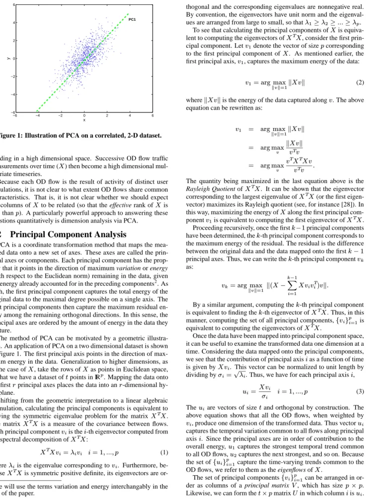
Figure 1: Illustration of PCA on a correlated, 2-D dataset.

residing in a high dimensional space. Successive OD flow traffic measurements over time (X) then become a high dimensional

mul-tivariate timeseries.

Because each OD flow is the result of activity of distinct user populations, it is not clear to what extent OD flows share common characteristics. That is, it is not clear whether we should expect the columns ofX to be related (so that the effective rank ofX is

less thanp). A particularly powerful approach to answering these

questions quantitatively is dimension analysis via PCA.

2.2 Principal Component Analysis

PCA is a coordinate transformation method that maps the mea-sured data onto a new set of axes. These axes are called the prin-cipal axes or components. Each prinprin-cipal component has the prop-erty that it points in the direction of maximum variation or energy (with respect to the Euclidean norm) remaining in the data, given the energy already accounted for in the preceding components2. As such, the first principal component captures the total energy of the original data to the maximal degree possible on a single axis. The next principal components then capture the maximum residual en-ergy among the remaining orthogonal directions. In this sense, the principal axes are ordered by the amount of energy in the data they capture.

The method of PCA can be motivated by a geometric illustra-tion. An application of PCA on a two dimensional dataset is shown in Figure 1. The first principal axis points in the direction of max-imum energy in the data. Generalization to higher dimensions, as in the case ofX, take the rows ofXas points in Euclidean space,

so that we have a dataset oftpoints in IR p

. Mapping the data onto the firstrprincipal axes places the data into anr-dimensional

hy-perplane.

Shifting from the geometric interpretation to a linear algebraic formulation, calculating the principal components is equivalent to solving the symmetric eigenvalue problem for the matrixX

T X.

The matrixX T

X is a measure of the covariance between flows.

Each principal componentviis thei-th eigenvector computed from

the spectral decomposition ofX T

X: X

T

Xvi=ivi i=1;:::;p (1)

whereiis the eigenvalue corresponding tovi. Furthermore,

be-causeX T

Xis symmetric positive definite, its eigenvectors are

or-2_{We will use the terms variation and energy interchangably in the}

rest of the paper.

thogonal and the corresponding eigenvalues are nonnegative real. By convention, the eigenvectors have unit norm and the eigenval-ues are arranged from large to small, so that

1

2

::: p.

To see that calculating the principal components ofXis

equiva-lent to computing the eigenvectors ofX T

X, consider the first

prin-cipal component. Letv

1denote the vector of size

pcorresponding

to the first principal component ofX. As mentioned earlier, the

first principal axis,v

1, captures the maximum energy of the data:

v 1

=argmax kvk=1

kXvk (2)

wherekXvkis the energy of the data captured alongv. The above

equation can be rewritten as:

v1 = arg max kvk=1 kXvk = argmax v kXvk v T v = argmax v v T X T Xv v T v :

The quantity being maximized in the last equation above is the

Rayleigh Quotient ofX T

X. It can be shown that the eigenvector

corresponding to the largest eigenvalue ofX T

X(or the first

eigen-vector) maximizes its Rayleigh quotient (see, for instance [28]). In this way, maximizing the energy ofXalong the first principal

com-ponentv

1is equivalent to computing the first eigenvector of X

T X.

Proceeding recursively, once the firstk 1principal components

have been determined, thek-th principal component corresponds to

the maximum energy of the residual. The residual is the difference between the original data and the data mapped onto the firstk 1

principal axes. Thus, we can write thek-th principal componentv k as: v k =argmax kvk=1 k(X k 1 X i=1 Xv i v T i )vk:

By a similar argument, computing thek-th principal component

is equivalent to finding thek-th eigenvector ofX T

X. Thus, in this

manner, computing the set of all principal components,fvig p i=1

is equivalent to computing the eigenvectors ofX

T X.

Once the data have been mapped into principal component space, it can be useful to examine the transformed data one dimension at a time. Considering the data mapped onto the principal components, we see that the contribution of principal axisias a function of time

is given byXvi. This vector can be normalized to unit length by

dividing by i

= p

i. Thus, we have for each principal axis i, ui= Xv i i i=1;:::;p (3) Theu

i are vectors of size

tand orthogonal by construction. The

above equation shows that all the OD flows, when weighted by

vi, produce one dimension of the transformed data. Thus vectorui

captures the temporal variation common to all flows along principal axisi. Since the principal axes are in order of contribution to the

overall energy,u1 captures the strongest temporal trend common

to all OD flows,u

2captures the next strongest, and so on. Because

the set offu i

g p i=1

capture the time-varying trends common to the OD flows, we refer to them as the eigenflows ofX.

The set of principal componentsfvig p i=1

can be arranged in or-der as columns of a principal matrixV, which has sizepp.

(4)

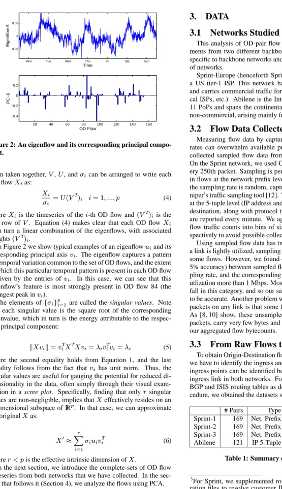
Mon Tue Wed Thu Fri Sat Sun −0.05 0 0.05 Time Eigenflow 6 20 40 60 80 100 120 140 160 −0.4 −0.2 0 0.2 OD Flow PC − 6

Figure 2: An eigenflow and its corresponding principal compo-nent.

Then taken together,V,U, andican be arranged to write each

OD flowX ias: X i i =U(V T )i i=1;:::;p (4) whereX

iis the timeseries of the

i-th OD flow and(V T

) iis the i-th row ofV. Equation (4) makes clear that each OD flowX

i

is in turn a linear combination of the eigenflows, with associated weights(V

T )

i.

In Figure 2 we show typical examples of an eigenflowu iand its

corresponding principal axisvi. The eigenflow captures a pattern

of temporal variation common to the set of OD flows, and the extent to which this particular temporal pattern is present in each OD flow is given by the entries ofvi. In this case, we can see that this

eigenflow’s feature is most strongly present in OD flow 84 (the strongest peak inv i). The elements off i g p i=1

are called the singular values. Note that each singular value is the square root of the corresponding eigenvalue, which in turn is the energy attributable to the respec-tive principal component:

kXvik=v T i X T Xvi=iv T i vi=i (5)

where the second equality holds from Equation 1, and the last equality follows from the fact thatvi has unit norm. Thus, the

singular values are useful for gauging the potential for reduced di-mensionality in the data, often simply through their visual exam-ination in a scree plot. Specifically, finding that onlyrsingular

values are non-negligible, implies thatXeffectively resides on an r-dimensional subspace of IR

p

. In that case, we can approximate the originalXas:

X 0 r X i=1 iuiv T i (6)

wherer<pis the effective intrinsic dimension ofX.

In the next section, we introduce the complete-sets of OD flow timeseries from both networks that we have collected. In the sec-tion that follows it (Secsec-tion 4), we analyze the flows using PCA.

3. DATA

3.1 Networks Studied

This analysis of OD-pair flow properties is based on measure-ments from two different backbone networks. However, it is not specific to backbone networks and can be applied to different types of networks.

Sprint-Europe (henceforth Sprint) is the European backbone of a US tier-1 ISP. This network has 13 Points of presence (PoPs) and carries commercial traffic for large customers (companies, lo-cal ISPs, etc.). Abilene is the Internet2 backbone network. It has 11 PoPs and spans the continental USA. The traffic on Abilene is non-commercial, arising mainly from major universities in the US.

3.2 Flow Data Collected

Measuring flow data by capturing every packet at high packet rates can overwhelm available processing power. Therefore, we collected sampled flow data from every router in both networks. On the Sprint network, we used Cisco’s NetFlow [5] to collect ev-ery 250th packet. Sampling is periodic, and results are aggregated in flows at the network prefix level, every 5 minutes. On Abilene, the sampling rate is random, capturing 1% of all packets using Ju-niper’s traffic sampling tool [12]. The monitored flow granularity is at the 5-tuple level (IP address and port number for both source and destination, along with protocol type) and sampled measurements are reported every minute. We aggregated the Sprint and Abilene flow traffic counts into bins of size 10 minutes and 5 minutes re-spectively to avoid possible collection synchronization issues.

Using sampled flow data has two major drawbacks. First, when a link is lightly utilized, sampling everyN-th packet undersamples

some flows. However, we found excellent agreement (within 1%-5% accuracy) between sampled flow bytecounts, adjusted for sam-pling rate, and the corresponding SNMP bytecounts on links with utlization more than 1 Mbps. Most of the links from both networks fall in this category, and so our sampled flow bytecounts are likely to be accurate. Another problem with measuring flows by sampling packets on any link is that some flows are not sampled altogether. As [8, 10] show, these unsampled flows have a small number of packets, carry very few bytes and so will have negligible impact on our aggregated flow bytecounts.

3.3 From Raw Flows to OD Flows

To obtain Origin-Destination flows from the raw flows collected, we have to identify the ingress and egress points of each flow. The ingress points can be identified because we collect data from each ingress link in both networks. For egress point resolution, we use BGP and ISIS routing tables as detailed in [2, 9]3. Using this pro-cedure, we obtained the datasets summarized in Table 1.

# Pairs Type Time Bin Period Sprint-1 169 Net. Prefix 10 min Jul 07-Jul 13 Sprint-2 169 Net. Prefix 10 min Aug 04-Aug 10 Sprint-3 169 Net. Prefix 10 min Aug 11-Aug 17 Abilene 121 IP 5-Tuple 5 min Apr 07-Apr 13

Table 1: Summary of datasets studied.

3

For Sprint, we supplemented routing tables with router configu-ration files to resolve customer IP address spaces. Also, Abilene anonymizes the last 11 bits of the destination IP. This is not a sig-nificant concern because there are few prefixes less than 11 bits in the Abilene routing tables, and we found very little traffic destined to these prefixes.

(5)

Mon Tue Wed Thu Fri Sat Sun 0.85 0.9 0.95 1 1.05 1.1 1.15 1.2 1.25 1.3 1.35 x 108 Traffic in OD Flow 84 Original 5 PC

Mon Tue Wed Thu Fri Sat Sun 0.5 1 1.5 2 2.5 x 107 Traffic in OD Flow 79 Original 5 PC

Mon Tue Wed Thu Fri Sat Sun 1 2 3 4 5 6 7 x 107 Traffic in OD Flow 96 Original 5 PC

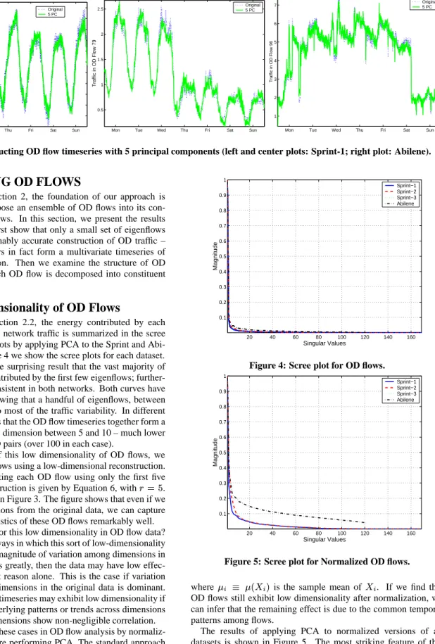
Figure 3: Reconstructing OD flow timeseries with 5 principal components (left and center plots: Sprint-1; right plot: Abilene).

4. ANALYZING OD FLOWS

As described in Section 2, the foundation of our approach is to use PCA to decompose an ensemble of OD flows into its con-stituent set of eigenflows. In this section, we present the results of that process. We first show that only a small set of eigenflows is necessary for reasonably accurate construction of OD traffic – meaning that OD flows in fact form a multivariate timeseries of low effective dimension. Then we examine the structure of OD flows, that is, how each OD flow is decomposed into constituent eigenflows.

4.1 Low Dimensionality of OD Flows

As described in Section 2.2, the energy contributed by each eigenflow to aggregate network traffic is summarized in the scree plot. We form scree plots by applying PCA to the Sprint and Abi-lene datasets. In Figure 4 we show the scree plots for each dataset. The figure shows the surprising result that the vast majority of traffic variability is contributed by the first few eigenflows; further-more, this effect is consistent in both networks. Both curves have a very sharp knee, showing that a handful of eigenflows, between 5 and 10, contribute to most of the traffic variability. In different terms, this result shows that the OD flow timeseries together form a structure with effective dimension between 5 and 10 – much lower than the number of OD pairs (over 100 in each case).

As an illustration of this low dimensionality of OD flows, we plot a sample of OD flows using a low-dimensional reconstruction. We do so by representing each OD flow using only the first five eigenflows. This construction is given by Equation 6, withr=5.

The results are shown in Figure 3. The figure shows that even if we omit over 100 dimensions from the original data, we can capture the temporal characteristics of these OD flows remarkably well.

What is the reason for this low dimensionality in OD flow data? There are at least two ways in which this sort of low-dimensionality can arise. First, if the magnitude of variation among dimensions in the original data differs greatly, then the data may have low effec-tive dimension for that reason alone. This is the case if variation along a small set of dimensions in the original data is dominant. Second, a multivariate timeseries may exhibit low dimensionality if there are common underlying patterns or trends across dimensions – in other words, if dimensions show non-negligible correlation.

We can distinguish these cases in OD flow analysis by normaliz-ing the OD flows before performnormaliz-ing PCA. The standard approach is to normalize each dimension to zero mean and unit variance. For OD flow data we have:

Xi=Xi i i=1;:::;p 20 40 60 80 100 120 140 160 0.1 0.2 0.3 0.4 0.5 0.6 0.7 0.8 0.9 1 Singular Values Magnitude Sprint−1 Sprint−2 Sprint−3 Abilene

Figure 4: Scree plot for OD flows.

20 40 60 80 100 120 140 160 0.1 0.2 0.3 0.4 0.5 0.6 0.7 0.8 0.9 1 Singular Values Magnitude Sprint−1 Sprint−2 Sprint−3 Abilene

Figure 5: Scree plot for Normalized OD flows.

wherei (Xi) is the sample mean ofXi. If we find that

OD flows still exhibit low dimensionality after normalization, we can infer that the remaining effect is due to the common temporal patterns among flows.

The results of applying PCA to normalized versions of all datasets is shown in Figure 5. The most striking feature of this figure is that the sharp knee from Figure 4 remains, in nearly the same location. It is also clear that the relative significance of the first few eigenflows has diminished somewhat.

(6)

20 40 60 80 100 120 140 160 0 0.1 0.2 0.3 0.4 0.5 0.6 0.7 0.8 0.9 1

Number of Eigenflows in an OD flow

Pr[X<x]

Sprint Abilene

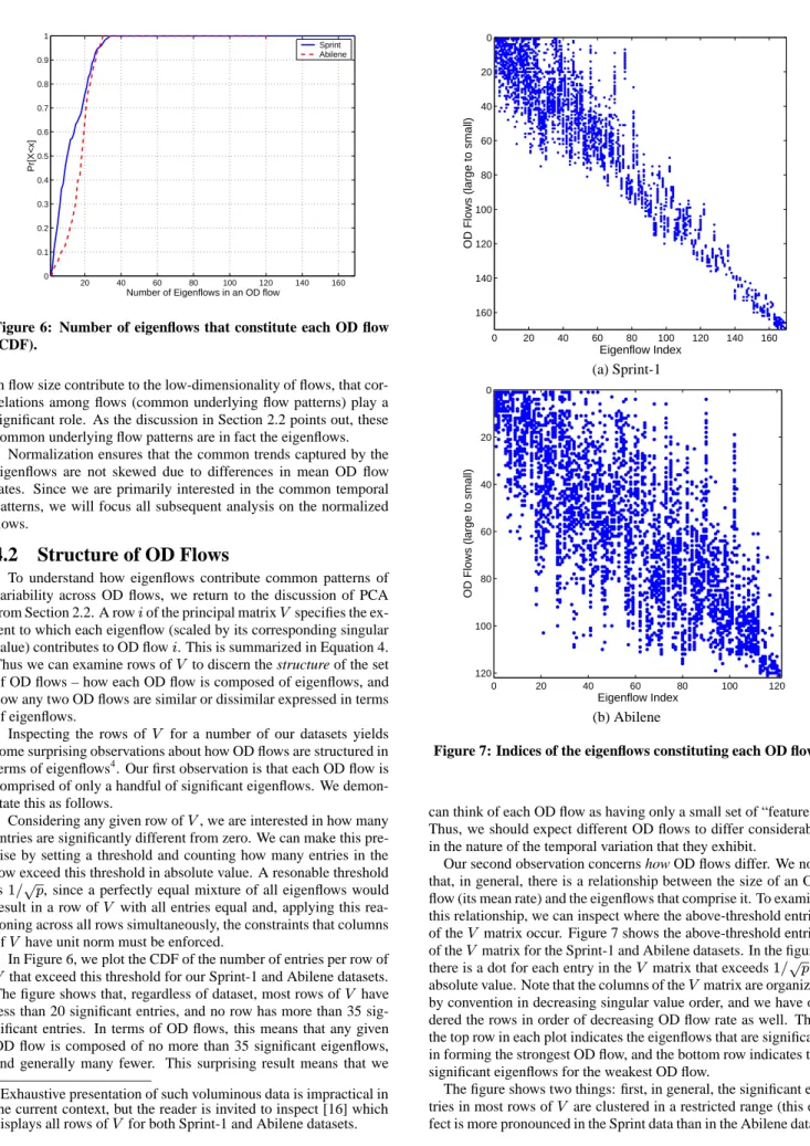
Figure 6: Number of eigenflows that constitute each OD flow (CDF).

in flow size contribute to the low-dimensionality of flows, that cor-relations among flows (common underlying flow patterns) play a significant role. As the discussion in Section 2.2 points out, these common underlying flow patterns are in fact the eigenflows.

Normalization ensures that the common trends captured by the eigenflows are not skewed due to differences in mean OD flow rates. Since we are primarily interested in the common temporal patterns, we will focus all subsequent analysis on the normalized flows.

4.2 Structure of OD Flows

To understand how eigenflows contribute common patterns of variability across OD flows, we return to the discussion of PCA from Section 2.2. A rowiof the principal matrixV specifies the

ex-tent to which each eigenflow (scaled by its corresponding singular value) contributes to OD flowi. This is summarized in Equation 4.

Thus we can examine rows ofV to discern the structure of the set

of OD flows – how each OD flow is composed of eigenflows, and how any two OD flows are similar or dissimilar expressed in terms of eigenflows.

Inspecting the rows ofV for a number of our datasets yields

some surprising observations about how OD flows are structured in terms of eigenflows4_{. Our first observation is that each OD flow is}

comprised of only a handful of significant eigenflows. We demon-state this as follows.

Considering any given row ofV, we are interested in how many

entries are significantly different from zero. We can make this pre-cise by setting a threshold and counting how many entries in the row exceed this threshold in absolute value. A resonable threshold is1=

p

p, since a perfectly equal mixture of all eigenflows would

result in a row ofV with all entries equal and, applying this

rea-soning across all rows simultaneously, the constraints that columns ofV have unit norm must be enforced.

In Figure 6, we plot the CDF of the number of entries per row of

V that exceed this threshold for our Sprint-1 and Abilene datasets.

The figure shows that, regardless of dataset, most rows ofV have

less than 20 significant entries, and no row has more than 35 sig-nificant entries. In terms of OD flows, this means that any given OD flow is composed of no more than 35 significant eigenflows, and generally many fewer. This surprising result means that we

4

Exhaustive presentation of such voluminous data is impractical in the current context, but the reader is invited to inspect [16] which displays all rows ofV for both Sprint-1 and Abilene datasets.

0 20 40 60 80 100 120 140 160 0 20 40 60 80 100 120 140 160 Eigenflow Index

OD Flows (large to small)

(a) Sprint-1 0 20 40 60 80 100 120 0 20 40 60 80 100 120 Eigenflow Index

(b) Abilene

Figure 7: Indices of the eigenflows constituting each OD flow.

can think of each OD flow as having only a small set of “features.” Thus, we should expect different OD flows to differ considerably in the nature of the temporal variation that they exhibit.

Our second observation concerns how OD flows differ. We note that, in general, there is a relationship between the size of an OD flow (its mean rate) and the eigenflows that comprise it. To examine this relationship, we can inspect where the above-threshold entries of theV matrix occur. Figure 7 shows the above-threshold entries

of theV matrix for the Sprint-1 and Abilene datasets. In the figure,

there is a dot for each entry in theV matrix that exceeds1= p

absolute value. Note that the columns of theV matrix are organized

by convention in decreasing singular value order, and we have or-dered the rows in order of decreasing OD flow rate as well. Thus the top row in each plot indicates the eigenflows that are significant in forming the strongest OD flow, and the bottom row indicates the significant eigenflows for the weakest OD flow.

The figure shows two things: first, in general, the significant en-tries in most rows ofV are clustered in a restricted range (this

(7)

Mon Tue Wed Thu Fri Sat Sun 0.022 0.024 0.026 0.028 0.03 0.032 0.034 0.036 0.038 Eigenflow 1

Mon Tue Wed Thu Fri Sat Sun

−0.06 −0.04 −0.02 0 0.02 0.04 Eigenflow 2

0.012 0.014 0.016 0.018 0.02 0.022 0.024 0.026 0.028 Eigenflow 1

−0.05 −0.04 −0.03 −0.02 −0.01 0 0.01 0.02 0.03 0.04 Eigenflow 2

−0.05 0 0.05 0.1 0.15 0.2 0.25 0.3 Eigenflow 8

−0.05 0 0.05 0.1 0.15 0.2 0.25 0.3 0.35 Eigenflow 20

−0.05 0 0.05 0.1 0.15 0.2 0.25 0.3 Eigenflow 6

−0.12 −0.1 −0.08 −0.06 −0.04 −0.02 0 0.02 0.04 0.06 Eigenflow 10

−0.1 −0.08 −0.06 −0.04 −0.02 0 0.02 0.04 0.06 0.08 Eigenflow 29

−0.1 −0.05 0 0.05 0.1 Eigenflow 39

−0.06 −0.04 −0.02 0 0.02 0.04 0.06 0.08 Eigenflow 49

−0.06 −0.04 −0.02 0 0.02 0.04 0.06 0.08 Eigenflow 53

(a) Sprint-1 (b) Abilene

Figure 8: Eigenflow examples. Top Row: Deterministic Eigenflows; Middle Row: Spike Eigenflows; Bottom Row: Noise Eigenflows.

Second, larger flows tend to be comprised mainly of the most sig-nificant eigenflows, and smaller flows tend to be comprised mainly of less significant eigenflows.

In some ways, the results shown in Figure 7 are not surprising. The largest OD flows will tend to dominate the definition of the most significant eigenflows, and so the steady upward trend in the plot is more or less to be expected. However the tight clustering of the significant eigenflows for any OD flow means that if there are qualitative differences between eigenflows in different ranges, then these qualitative differences will be reflected in the OD flows. Indeed, in the next section we show that this is in fact the case.

5. UNDERSTANDING EIGENFLOWS

The analysis of OD flows presented in the last section has em-phasized the central role of eigenflows in understanding OD flow properties. Thus we turn now to eigenflows; we inspect them, de-scribe the three types most often seen, and show how understanding those types in light of the results in the previous section can yield general insight into OD flow properties.

5.1 A Taxonomy of Eigenflows

We start by inspecting the complete sets of eigenflows for a number of our datasets5_{. Surprisingly, across all of the}

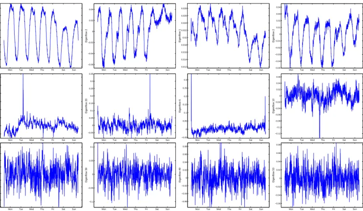
eigen-flows we examined, there appear to be only three distinctly dif-ferent types. Representative examples of each eigenflow type from both the Sprint-1 and Abilene datasets are shown in Figure 8.

The top row shows examples of eigenflows that exhibit strong

5

As in Section 4.2, the raw data is too voluminous to present, but plots of the complete set of eigenflows for both datasets are avail-able at [16].

periodicities. The periodicities clearly reflect diurnal activity, as well as the difference between weekday and weekend activity. Be-cause these eigenflows appear to be relatively predictable, we refer to them as d-eigenflows (for “deterministic”).

The second row of Figure 8 shows examples of eigenflows that exhibit strong, short-lived spikes. These s-eigenflows (for “spike”) show isolated values that can be many standard deviations (e.g., 4 or 5 standard deviations) from the eigenflow mean. These clearly capture the occasional traffic bursts and dips that are a common feature of network data traffic.

Finally, the lowest row of Figure 8 shows examples of eigenflows that appear roughly stationary and Gaussian. These n-eigenflows (for “noise”) capture the remaining random variation that arises as the result of multiplexing many individual traffic sources. The ma-jority of eigenflows in both datasets appear to be of this type.

These categories of eigenflows are only heuristically distin-guished. It is not our intent to suggest that any eigenflow can be unambiguously categorized in this manner. Nonetheless, we ob-serve that these categories are in fact very distinct, and that almost all eigenflows can be easily placed into one of these categories.

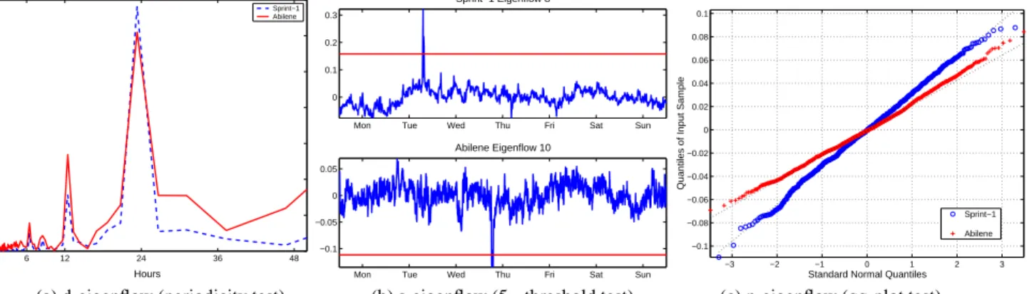
To demonstrate that these categories are distinct and that most eigenflows fall clearly into one of the three categories, we evaluate each flow according to the following criteria:

1. Does the eigenflow have a strong peak in its Fourier spectrum at 12 or 24 hours? A strong peak is defined here as a power value at that frequency greater than any other value in the power spectrum.

2. Does the eigenflow contain at least one outlier that exceeds 5 standard deviations from its mean?

(8)

0 6 12 24 36 48 0 0.5 1 1.5 2 2.5 3 3.5 Hours FFT Energy Sprint−1 Abilene

Mon Tue Wed Thu Fri Sat Sun 0

0.1 0.2 0.3

Sprint−1 Eigenflow 8

Mon Tue Wed Thu Fri Sat Sun −0.1 −0.05 0 0.05 Abilene Eigenflow 10 −3 −2 −1 0 1 2 3 −0.1 −0.08 −0.06 −0.04 −0.02 0 0.02 0.04 0.06 0.08 0.1

Standard Normal Quantiles

Quantiles of Input Sample

Sprint−1 Abilene

(a) d-eigenflow (periodicity test) (b) s-eigenflow (5threshold test) (c) n-eigenflow (qq-plot test)

Figure 9: Classifying eigenflows by using three tests.

to be nearly Gaussian? We judge whether an eigenflow meets this criterion by examining its distribution on a qq-plot, which plots quantiles of the data against quantiles of the Normal distribution; a straight line indicates a close fit of the data to the Normal.

Examples of applying these criteria to eigenflows from both datasets are shown in Figure 9. Figure 9(a) shows that the eigen-flows that we visually identify as d-eigeneigen-flows indeed have a dis-tinct power spectrum peak at 24 hours. In Figure 9(b) we show visually identified s-eigenflows that have 5-sigma excursions from the mean. And in Figure 9(c) we show eigenflows that are visually categorized as n-eigenflows appear to have marginal distributions that are nearly Gaussian.

We used these tools to examine all eigenflows from both datasets6. Eigenflows for which more than one of the criterion above held true were categorized as “indeterminate.” In the Sprint-1 dataset, only 4 were indeterminate (contributing 0.0Sprint-12% to over-all energy); in the Abilene dataset, only 2 were indeterminate (con-tributing 0.26% to overall energy). For all of the remaining eigen-flows, one and only one criterion above held true.

Thus, by using the criteria above, we can (again, heuristically) place almost every eigenflow into one of the three categories. When we do so, we find that we can obtain considerable insight into the properties of the OD flows.

A clear benefit of this categorization is that it cleanly decom-poses any given OD flow into its principal features. That is, we can reconstruct each OD flow in terms of three constituents: the con-tributions made by d-eigenflows, s-eigenflows, and n-eigenflows. When we do so, each constituent tends to capture a distinct fea-ture of the OD flow: its (deterministic) mean, its sharp bursts away from the mean, and its apparently-stationary random variation. An example of this decomposition is shown in Figure 10. The figure shows the original flow along with its three constituent features as captured by its component eigenflows. The separation of bursts and random noise from the nonstationary variation of the mean is quite sharp. Furthermore, the isolation of bursts from background noise is also quite distinct. While a similar result could likely have been obtained by applying (probably sophisticated) timeseries models, we note that we have made no modeling assumptions here other than the simple categorization of eigenflows. Rather, the power be-hind this method comes from the extraction of common variation patterns across OD flows as the information needed to identify and separate different kinds of variability within a single OD flow.

6

Plots similar to Figure 9 for each eigenflow can be found at [16].

1 1.5 2 x 107 Original 0.6 0.8 1 1.2 1.4 1.6 1.8 x 107 d−eigenflows −5 0 5 x 106 s−eigenflows

−5 0 5

x 106

n−eigenflows

Figure 10: Decomposition of OD flow timeseries into the sum of its three constituent eigenflows.

The features isolated in distinct eigenflows conform to charac-teristics that have been found in studies of other network traf-fic. Specifically, the presence of diurnal trends has been noted in [21, 25] for SNMP link data, the presence of stochastic bursts has been found in IP flow data by [26] and finally, the well-known fractional gaussian noise structure was first found in link level traf-fic by [17]. While previous studies have generally concentrated on identifying and describing these features from a model-based standpoint, this result shows that systematically isolating the com-mon patterns of flow variability without recourse to elaborate mod-eling results in essentially the same set of features.

Given the apparent power deriving from categorizing eigenflows, it is worth investigating the relative role that the three types play in decomposing OD traffic. As a first step, we note that the different eigenflow types appear in different regions when the eigenflows are ordered by overall importance (i.e., by singular value). To illustrate this effect, we show in Figure 11 the classification for each eigen-flow in the Sprint-1 and Abilene datasets. The figure shows that in both datasets, d-eigenflows mainly appear as approximately the first six eigenflows. The next 5-6 eigenflows in order tend to be

(9)

Eigenflow type Sprint-1 Abilene d-eigenflow 92.17% 69.79% s-eigenflow 5.59% 18.60% n-eigenflow 2.24% 11.61%

Table 2: Contribution of eigenflow type to overall traffic.

s-eigenflows. The only difference between the datasets is in nature of the least significant eigenflows (eigenflows numbered 12 and be-yond): in Abilene, the least significant eigenflows are almost all of the noise type, while in Sprint-1 the least significant eigenflows are more spike-type than noise. We leave an exploration of these dif-ferences for future work.

Figure 11 provides insight into the relative roles played by differ-ent sources of variability in our OD flow data. The figure shows that the most important source of variation is the nonstationary changes in the mean due to periodic trends. After these periodic trends, traffic bursts or spikes are next in importance. Finally, the least significant contribution to traffic variability in these datasets comes from noise. These conclusions are confirmed in a more quantitative way by the data in Table 2, which shows the fraction of total energy in each dataset that can be assigned to each of the three eigenflow types.

20 40 60 80 100 120 140 160

d−eigenflow s−eigenflow n−eigenflow

Sprint Eigenflows in order

20 40 60 80 100 120

d−eigenflow s−eigenflow n−eigenflow

Abilene Eigenflows in order

Figure 11: Occurence of eigenflow type in order of importance. Top: Sprint-1; Bottom: Abilene.

5.2 Decomposing OD Flows

We can refine our understanding of the nature of variability in OD traffic by using this categorization of eigenflows to decompose each OD flow. Such a decomposition of OD flows gives insight into how traffic features vary from one OD flow to the next.

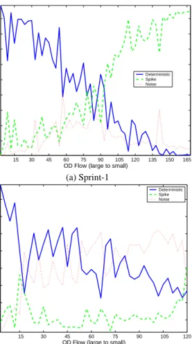
To do so, we determine the relative contribution of each eigen-flow type to each OD eigen-flow. The results are shown in Figure 12. In this figure, OD flows are ordered by mean rate, decreasing from left to right. For each flow we plot the fraction of its energy contributed by d-, s-, and n-eigenflows. (We have averaged adjacent values in this figure to improve legibility.)

The figure shows that the PCA based decomposition of OD flows exposes how the properties of OD flows vary. We can see that high-volume OD flows are dominated by periodic, deterministic trends. As we move to the right of the figure, the relative contribution of

15 30 45 60 75 90 105 120 135 150 165 0.1 0.2 0.3 0.4 0.5 0.6 0.7 0.8 0.9

Fraction of Total Energy

OD Flow (large to small)

Deterministic Spike Noise (a) Sprint-1 15 30 45 60 75 90 105 120 0.1 0.2 0.3 0.4 0.5 0.6 0.7 0.8

Fraction of Total Energy

OD Flow (large to small)

Deterministic Spike Noise

(b) Abilene

Figure 12: Fraction of total energy captured by eigenflow type for all OD flows.

deterministic components decreases, and a distinction in the struc-ture of OD flows from the two networks emerges. For Sprint, we find that the lower-volume an OD flow, the more it tends to be dom-inated entirely by spikes. And, regardless of the volume of the OD flow, a relatively constant proportion of its energy can be attributed to noise. On the other hand, the lower volume Abilene flows are dominated by noise and some periodic trends. Furthermore, regard-less of the volume of the OD flow, a relatively constant proportion of its energy is due to traffic bursts. Thus, we can relate the statis-tical properties (temporal features) of an OD flow in a particularly simple way to the flow’s overall traffic volume.

These results provide a powerful organizing tool for thinking about collections of OD flows. They draw attention to the signif-icant statistical differences between high-volume and low-volume OD flows and between the structure of traffic in different networks. They suggest that a simple model may not be appropriate for all OD flows across a network. And they allow researchers and en-gineers to relate the properties of OD flows to the nature of the source and destination user or customer populations, through those populations’ influences on OD flow traffic volume.

6. TEMPORAL

STABILITY OF

FLOW

STRUCTURE

The previous sections have shown that PCA can unearth impor-tant structure in OD flow data. For many practical applications, it

(10)

will be important to know the extent to which this structure varies in time.

The question we are concerned with in this section is whether the decomposition of OD flows into eigenflows, as determined by the set of pricipal components, is useful for analyzing data that was not part of the input to the PCA procedure. In general, we envision applications that may benefit from using PCA in an on-line manner as follows. Given OD flow data observed over some time period[t

0 ;t

1

), obtain the principal componentsfv i

g.

Subse-quently, at some timet2 > t1, usefvigto decompose a new set

of OD flow observations into eigenflows. Does the subsequent de-composition preserve useful properties of the eigenflows? We can ask two specific versions of this question: First, does the subse-quent decomposition still have relatively low effective dimension-ality? And second, if the original decomposition has categorized eigenflows by type, is that categorization still useful in the subse-quent decomposition? Although space does not permit us to answer these questions thoroughly, we give some initial results here.

To answer the first question, we proceed as follows. One way to assess whether a set of OD flows has low effective dimension is to measure the error resulting from approximating the set of flows us-ing a small number of dimensions. Usus-ing two consecutive weeks of OD flow dataX1andX2, we start by analyzingX1using PCA and

obtaining its pricipal componentsfvig. We usefvigto construct

the top 20 eigenflows forX

1, and we also use fv

i

gin the same way

to construct a corresponding set of 20 pseudo-eigenflows forX2.

We use the term pseudo-eigenflows for the linear combinations of the OD flows ofX

2obtained using the fv

i gofX

1, to remind us

that they are not the result of applying PCA directly toX

2, but may

still approximately have the desirable properties of the eigenflows ofX

2. In each case, we form approximate versions of the

origi-nal data using only the top 20 pseudo-eigenflows, yieldingX 0 1and X

0 2

:We then measure the per-flow sum of squared error of each

approximation: SSE1=jjX1 X 0 1 jj and SSE2 =jjX2 X 0 2 jj

and the mean relative error of each approximation:

R1=avg(jX1 X 0 1 j=X1) and R2=avg(jX2 X 0 2 j=X2):

Based on the results in Section 4.1, we expect the error forX 1

to be small in general, because we know that OD flows can be ac-curately approximated using a small number of eigenflows. Fur-thermore, we expect the per-flow error forX

2to be larger than the

corresponding error forX1, since thefvigused in approximating X2were not necessarily optimal. However, what is not clear is how

much worse the error will be forX

2than for X

1.

We performed this analysis on datasets from the Sprint network, withX1consisting of data for the week of 04 August to 10 August

(Sprint-2 dataset) andX

2consisting of data for the next week, i.e.,

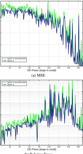
11 August to 17 August (Sprint-3 dataset). The results are shown in Figure 13. Figure 13(a) shows the sum of squared error per OD flow, with flows ordered by decreasing mean rate from left to right. Figure 13(b) shows the mean relative error per OD flow.

The plots show that overall, the error induced by using the pre-vious week’s principal components to analyze the current week’s OD flows is not great. The relative approximation error forX

1for

the 20 or so heaviest (most important) flows is in the range of 5%. The relative approximation error forX

2, using the principal

com-ponents ofX

1, is in the range (for the same flows) of approximately

10%. Thus, the first week’s principal components appear to remain good choices for forming a low-dimensional representation of the subsequent consecutive week.

The second question we ask is whether the categorization of

20 40 60 80 100 120 140 160 104 106 108 1010 1012

Mean Squared Error (log)

Sprint−3 reconstructed Sprint−2 (a) MSE 20 40 60 80 100 120 140 160 10−2 10−1 100 101 102 103

Relative Error (log)

Sprint−3 reconstructed Sprint−2

(b) Relative Error

Figure 13: Exploring the temporal stability of Principal Com-ponents.

eigenflows remains consistent enough from week to week to be use-ful. To answer this question we again decomposeX2into

pseudo-eigenflows, and we designate a pseudo-eigenflow a d-eigenflow if it was a d-eigenflow in the decomposition ofX

1. This allows us

to “detrend”X2without applying PCA to it directly. Detrending a

particular set of flows is then accomplished through a simple matrix multiplication.

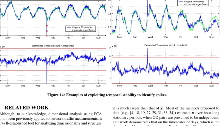
To illustrate the effectiveness of this online style of detrending, we use it to identify unusual events inX2. The approach is shown

in Figure 14. On the top of the figure are plots of two OD flows taken fromX

2. Below each OD flow we show the same OD flow

with deterministic components, as identified using the decompo-sition ofX

1, removed. The result of removing the deterministic

components appears to be a timeseries without much variation in mean, and therefore suitable for simple thresholding to identify un-usual events. We adopt the arbitrary threshold of 4 standard devia-tions; based on this theshold, we show that unusual events (values far from the mean) can be easily identified in the original OD flow. Taken together, these results suggest that the useful properties obtained from decomposition into eigenflows show a degree of sta-bility from week to week that may be useful. While further inves-tigation is needed to determine the extent in time over which such properties are stable for any given application, we believe that the results shown here are promising.

(11)

Mon Tue Wed Thu Fri Sat Sun 2 4 6 8 10

x 107 Original Timeseries for OD Flow# 84

Original Timeseries d pseudo−eigenflows

−2 −1.5 −1 −0.5 0 0.5 1

x 107 Detrended Timeseries with 4σ threshold

1 1.5 2 2.5 3 3.5x 10

7 Original Timeseries for OD Flow# 57

Original timeseries d−pseudo−eigenflows

−5 0 5 10

15x 10

6 Detrended Timeseries with 4σ threshold

Figure 14: Examples of exploiting temporal stability to identify spikes.

7. RELATED WORK

Although, to our knowledge, dimensional analysis using PCA has not been previously applied to network traffic measurements, it is a well-established tool for analyzing dimensionality and structure in other disciplines. Areas where it has been successfully employed in this way include face recognition [13], brain imaging [30], me-teorology [23] and fluid dynamics [15].

Modeling traffic timeseries on a single link has attracted con-siderable research. Examples of recent studies that characterize timeseries of link traffic in backbone networks over long timescales are [24, 25].

In contrast, there is little prior work on OD flows, despite their engineering importance. Directly measuring OD flows requires ad-ditional and intensive monitoring on many routers, a task that de-mands considerable resources for high speed networks. Recently, however, network operators and researchers have started to use sampling schemes to measure OD flows [9]. It is the recent avail-ability of such data that makes a study like ours now possible.

Two measurement studies that depart from the link-level traffic characterization and examine inter-PoP flows in a commercial Tier-1 backbone instead are [2, 9]. The authors of [2] observed many different types of OD flows, which behaved differently depending on link speed, type of relationship (peer or customer) and popular-ity. The implication is that it is difficult to devise a single model (or even a family of models) that characterizes a general PoP to PoP level flow.

Although there is little work that is closely related to ours, the work we report here has implications for a number of related net-working problems. Our principal results (low dimensionality of OD flows, and differences in OD flow characteristics based on rate) can inform other work in a number of contexts. Here we briefly contrast our proposed approach with existing methods for a few candidate problems.

Traffic Matrix Estimation: The traffic matrix estimation problem,

as originally formulated in [31], is an ill-posed linear inverse prob-lem of the formy=Ax, where one seeks to estimatex, the vector

of OD flows, giveny, the vector of link traffic, and the routing

matrixA(as defined in Section 2.1). The central difficulty of this

problem stems from the fact that the apparent dimensionalilty of

xis much larger than that ofy. Most of the methods proposed to

date (e.g., [4, 18, 19, 27, 29, 31, 33, 34]) estimatexover hour-long

stationary periods, when OD pairs are presumed to be independent. Our work demonstrates that on the timescales of days, which is the timescale of interest for many applications of traffic engineering, the effective dimensionality of OD flows is much smaller. In such scenarios therefore, the traffic matrix estimation problem may be more tractable and yield to direct solution methods.

Anomaly detection in timeseries: Anomalies in OD flow

time-series are difficult to identify without manual inspection. Simple thresholding schemes cannot be applied because the timeseries are nonstationary. A number of change detection methods have been proposed that rely on wavelet denoising techniques [1] and devi-ations from forecasted behavior [3, 14] to identify outliers. An alternative approach is to detrend the flow timeseries using its d-eigenflows and then perform simple threshold tests on the resulting timeseries. The elements of this approach were briefly examined in Section 6 (Figure 14).

Traffic Forecasting: The state of the art in traffic forecasting for IP

networks relies on forecasting models built on predictable trends of traffic, which are in turn isolated using wavelets [21]. An alterna-tive approach to a wavelet-based isolation of trends in an OD flow is to simply use its d-eigenflows. Having done so, we can build forecasting models for the d-eigenflows and forecast the traffic for the entire set of OD flows. An advantage of such a PCA-based ap-proach is that it allows simultaneous examination and forecasting of the entire ensemble of OD flow timeseries.

Traffic Engineering: The finding that large OD flows are mainly

periodic and small OD flows are predominantly noise has been ob-served by others anecdotally [33]. Using PCA, we can system-atically evaluate this effect with a fair amount of precision. An understanding of the structure of collections of OD flows has use in traffic engineering tasks, such as identifying the predictable and heaviest flows [20].

An investigation of some of these problems constitutes our ongoing work.

(12)

8. CONCLUSIONS

In this paper, we have analyzed the structure of complete sets of Origin-Destination flow timeseries from two different networks: the European Sprint backbone network and the Abilene Internet2 backbone.

The first question we asked was whether complete sets of OD flows can be captured with low dimensional representations. Prior work suggested that because OD flows number on the order of hun-dreds in medium-sized networks and because each OD flow serves a different customer population, they are complicated structures to collectively model. Using Principal Component Analysis, we found that the hundreds of OD flows from both networks can be accurately described in time using 5-10 independent dimensions.

This surprising low dimensionality motivated us to ask a second question: how best can we understand the ways in which an en-semble of OD flows are similar and the ways in which they differ. We found that by examining the eigenflows, which are the com-mon patterns of variation underlying OD flows, we could develop considerable understanding of the structure of OD flows. We found that the set of OD flows shows three features: deterministic trends, spikes and noise. Furthermore, the largest OD flows most strongly exhibit deterministic trends and the smallest OD flows are domi-nated by noise (for Abilene) and spikes (for Sprint). Thus using PCA, we were able to quantitatively decompose the structure of each OD flow into its constitutent features.

Our last objective was to examine the extent to which the struc-ture of OD flows unearthed by PCA varies over time. We found using the results of PCA of a previous week to decompose the structure of OD flows in the current week introduced very little error. Thus, the low-dimensional coordinate space formed by PCA shows some evidence of stability over time.

9. ACKNOWLEDGEMENTS

We are grateful to Rick Summerhill, Mark Fullmer (Internet 2), Matthew Davy (Indiana University) for helping us collect and un-derstand the flow measurements from Abilene. At Sprint, we thank Bjorn Carlsson, Jeff Loughridge, and Richard Gass for instrument-ing and collectinstrument-ing the Sprint NetFlow measurements. Finally, we thank Supratik Bhattacharyya (Sprint Labs) and Kav´e Salamatian (LIP 6) for helpful discussions.

10. REFERENCES

[1] P. Barford, J. Kline, D. Plonka, and A. Ron. A signal analysis of network traffic anomalies. In Internet Measurement Workshop, Marseille, November 2002. [2] S. Bhattacharyya, C. Diot, J. Jetcheva, and N. Taft. Pop-Level and

Access-Link-Level Traffic Dynamics in a Tier-1 POP. In Internet Measurement Workshop, San Francisco, November 2001.

[3] J. Brutlag. Aberrant behavior detection in timeseries for network monitoring. In USENIX LISA, New Orleans, December 2000.

[4] J. Cao, D. Davis, S. V. Weil, and B. Yu. Time-Varying Network Tomography. J. of the American Statistical Association, pages 1063–1075, 2000.

[5] Cisco NetFlow. At

www.cisco.com/warp/public/732/Tech/netflow/. [6] M. Crovella and E. Kolaczyk. Graph Wavelets for Spatial Traffic Analysis. In

IEEE INFOCOM, San Francisco, April 2003.

[7] D. Donoho. High-Dimensional Data Analysis: The Curses and Blessings of Dimensionality. In American Math. Society. Available at:

www-stat.stanford.edu/˜donoho/Lectures/AMS2000/, 2000.

[8] N. Duffield, C. Lund, and M. Thorup. Estimating Flow Distributions from Sampled Flow Statistics. In ACM SIGCOMM, Karlsruhe, August 2003. [9] A. Feldmann, A. Greenberg, C. Lund, N. Reingold, J. Rexford, and F. True.

Deriving traffic demands for operational IP networks: Methodology and experience. In IEEE/ACM Transactions on Neworking, pages 265–279, June 2001.

[10] N. Hohn and D. Veitch. Inverting Sampled Traffic. In Internet Measurement Conference, Miami, October 2003.

[11] H. Hotelling. Analysis of a complex of statistical variables into principal components. J. Educ. Psy., pages 417–441, 1933.

[12] Juniper Traffic Sampling. At

www.juniper.net/techpubs/software/junos/junos60/ swconfig60-policy/html/%sampling-overview.html. [13] M. Kirby and L. Sirovich. Application of the Karhunen-Lo`eve procedure for the

characterization of human faces. IEEE Trans. Pattern Analysis and Machine Intelligence, pages 103–108, 1990.

[14] B. Krishnamurthy, S. Sen, Y. Zhang, and Y. Chen. Sketch-based Change Detection: Methods, Evaluation, and Applications. In Internet Measurement Conference, Miami, October 2003.

[15] L. Sirovich and K. S. Ball and L. R. Keefe. Plane Waves and Structures in Turbulent Channel Flow. Phys. Fluids. A, page 2217:2226, 1990. [16] A. Lakhina, K. Papagiannaki, M. Crovella, C. Diot, E. D. Kolaczyk, and

N. Taft. Analysis of Origin Destination Flows (Raw Data). Technical Report BUCS-2003-022, Boston University, 2003.

[17] W. Leland, M. Taqqu, W. Willinger, and D. Wilson. On the Self-Similar Nature of Ethernet Traffic (Extended Version). Transactions on Networking, pages 1–15, Feburary 1994.

[18] A. Medina, N. Taft, K. Salamatian, S. Bhattacharyya, and C. Diot. Traffic Matrix Estimation: Existing Techniques and New Directions. In ACM SIGCOMM, Pittsburgh, August 2002.

[19] A. Nucci, R. Cruz, N. Taft, and C. Diot. Design of IGP Link Weight Changes for Traffic Matrix Estimation. In IEEE INFOCOM, Hong Kong, April 2004. [20] K. Papagiannaki, N. Taft, and C. Diot. Impact of Flow Dynamics on Traffic

Engineering Design Principles. In IEEE INFOCOM, Hong Kong, April 2004. [21] K. Papagiannaki, N. Taft, Z. Zhang, and C. Diot. Long-Term Forecasting of

Internet Backbone Traffic: Observations and Initial Models. In IEEE INFOCOM, San Francisco, April 2003.

[22] V. Paxson and S. Floyd. Wide Area Traffic: The Failure of Poisson Modeling. Transactions on Networking, pages 236–244, June 1995.

[23] R. W. Preisendorfer. Principal Component Analysis in Meteorology and Oceanography. Elsevier, 1988.

[24] M. Roughan and J. Gottlieb. Large scale measurement and modeling of backbone internet traffic. In SPIE ITCom, Boston, August 2002. [25] M. Roughan, A. Greenberg, C. Kalmanek, M. Rumsewicz, J. Yates, and

Y. Zhang. Experience in measuring backbone traffic variability: Models, metrics, measurements and meaning. In International Teletraffic Conference (ITC-18), Berlin, September 2003.

[26] S. Sarvotham, R. Riedi, and R. Baraniuk. Network Traffic Analysis and Modeling at the Connection Level. In Internet Measurement Workshop, San Francisco, November 2001.

[27] A. Soule, A. Nucci, E. Leonardi, R. Cruz, and N. Taft. How to Identify and Estimate the Largest Traffic Matrix Elements in a Dynamic Environment. In ACM SIGMETRICS, New York, June 2004.

[28] G. Strang. Linear Algebra and its Applications. Thomson Learning, 1988. [29] C. Tebaldi and M. West. Bayesian Inference of Network Traffic Using Link

Data. J. of the American Statistical Association, pages 557–573, June 1998. [30] D. T’so, R. D. Frostig, E. E. Lieke, and A. Grinvald. Functional Organization of

primate visual cortex revealed by high resolution optical imaging. Science, pages 417–420, 1990.

[31] Y. Vardi. Network Tomography: Estimating Source-Destination Traffic Intensities from Link Data. J. of the American Statistical Association, pages 365–377, 1996.

[32] V. Yegneswaran, P. Barford, and J. Ullrich. Internet Intrusions: Global Characteristics and Prevalence. In ACM SIGMETRICS, San Diego, June 2003. [33] Y. Zhang, M. Roughan, N. Duffield, and A. Greenberg. Fast Accurate

Computation of Large-Scale IP Traffic Matrices from Link Loads. In ACM SIGMETRICS, San Diego, June 2003.

[34] Y. Zhang, M. Roughan, C. Lund, and D. Donoho. An Information-Theoretic Approach to Traffic Matrix Estimation. In ACM SIGCOMM, Karlsruhe, August 2003.