TKK Reports in Information and Computer Science
Espoo 2010 TKK-ICS-R34
USING MULTIPLE RE-EMBEDDINGS FOR QUANTITATIVE
STEGANALYSIS AND IMAGE RELIABILITY ESTIMATION
TKK Reports in Information and Computer Science
Espoo 2010 TKK-ICS-R34
USING MULTIPLE RE-EMBEDDINGS FOR QUANTITATIVE
STEGANALYSIS AND IMAGE RELIABILITY ESTIMATION
Yoan Miche, Patrick Bas and Amaury Lendasse
Aalto University School of Science and Technology Faculty of Information and Natural Sciences Department of Information and Computer Science
Aalto-yliopiston teknillinen korkeakoulu Informaatio- ja luonnontieteiden tiedekunta Tietojenka¨sittelytieteen laitos
Distribution:
Aalto University School of Science and Technology Faculty of Information and Natural Sciences Department of Information and Computer Science PO Box 15400 FI-00076 AALTO FINLAND URL: http://ics.tkk.fi Tel. +358 9 470 01 Fax +358 9 470 23369 E-mail: [email protected]
c Yoan Miche, Patrick Bas and Amaury Lendasse
ISBN 978-952-60-3249-8 (Print) ISBN 978-952-60-3250-4 (Online) ISSN 1797-5034 (Print) ISSN 1797-5042 (Online) URL: http://lib.tkk.fi/Reports/2010/isbn9789526032504.pdf TKK ICS Espoo 2010
ABSTRACT: The quantitative steganalysis problem aims at estimating the amount of payload embedded inside a document. In this paper, JPEG im-ages are considered, and by the use of a re-embedding based methodology, it is possible to estimate the number of original embedding changes performed on the image by a stego source and to slightly improve the estimation regard-ing classical quantitative steganalysis methods. The major advance of this methodology is that it also enables to obtain a confidence interval on this estimated payload. This confidence interval then permits to evaluate the dif-ficulty of an image, in terms of steganalysis by estimating the reliability of the output. The regression technique comes from the OP-ELM and the relia-bility is estimated using linear approximation. The methodology is applied with a publicly available stego algorithm, regression model and database of images. The methodology is generic and can be used for any quantitative steganalysis problem of this class.
KEYWORDS: Steganography, Steganalysis, OP-ELM, Quantitative Steganal-ysis, Re-embedding, Inner Image Difficulty
CONTENTS
1 Introduction 7
2 Methodology 8
2.1 Re-embedding concept . . . 9 2.2 Confidence interval estimation . . . 12 2.3 Estimation of the inner image difficulty . . . 12
3 Results 13
3.1 Estimation of the original embedding rateRˆo . . . 14 3.2 On the use of the width of the confidence interval . . . 16
4 Conclusion 18
References 18
1 INTRODUCTION
The classical goal of steganalysis is to detect whether a document (considered to be images, here) has been tampered with or not. While this detection is important, one can wish to obtain more information about the actual payload present in the image. This problem is addressed by quantitative steganalysis: it estimates the embedded payload, usually by estimating directly the number of embedding changes that have been made to the image in the first place. An initial approach to this has been proposed in [6, 13]. Such a problem has been addressed recently for example by the use of classical blind steganaly-sis features such as [5]: the knowledge of the stego algorithm is supposed to be given, following Kerckhoff’s principles [8] — or inferred by some usual means of blind steganalysis [11, 12] for example —, and the problem of pay-load estimation comes down to a regression problem, with the output being the payload to predict and inputs being the blind steganalysis features. In a recent paper, this regression has been achieved through the use of Ordinary Least Squares (OLS) and Support Vector Regression (SVR) [13].
In such a setup, it is assumed that one can use the identified stego al-gorithm in order to train an OLS or SVR model, for example on a known dataset. Such a model can then be used on new unknown images (the in-tercepted images on a specific channel) to estimate a possible embedded payload.
Although this usually leads to a good estimation, it is interesting to also have a confidence interval on such estimation, which gives information on the quality of the estimation as well as the possible “difficulty” of the consid-ered image (reliability), i.e. the reliability of the output.
This problem of image reliability is important for future steganography. Indeed, in the case where a specific image is known to be “difficult”, a steganographer will prefer using it, knowing that it is more likely to be mis-classified or have a payload estimation that is unreliable. In [14], the authors propose to estimate the embedding capacity of the image beforehand, in or-der to embed the payload into the possibly most appropriate images. Such an approach, combined with reliability estimation can lead to more secure steganography. For example, the estimation of the difficulty of the image could be a starting point to perform batch steganography by embedding a payload function of the difficulty of the image.
This idea of image difficulty was first related to the error in steganaly-sis in the work of Böhme [2]. In this paper, the authors define a two-error model for the quantitative steganalysis setup, with awithin-image error and abetween-image one. The between-image error relates to the possible inac-curate assumptions made on the cover image and is thus related to images as a whole.
The within-image error is highly related to the concept of difficulty used in this paper and attempts to take into account the errors caused by the possible dependencies between a cover image and the message embedded in it.
In the original paper, the authors illustrate through the use of numerous types of steganalysis on a LSB replacement steganography scheme that the between-image error and the within-image error are quite different in nature: the between-image error follows rather closely that of a Student’st
tion, while the within-image error is similar to a Gaussian one. It also seems that some of the steganalysis schemes tested by the authors are more prone to one type of error than the other.
The within-image error is related in [2] to a measure of the local variance of the image, introduced in the paper and computed over the original im-age. The concept of difficulty and the measure for it proposed in section 2 are tightly related to the within-image error and uses multiple repetitions of steganography with different messages on the same image. One main differ-ence here is that a blind approach is used to determine it, i.e. it is assumed that the original image is not available and it is only possible to rely on the intercepted suspicious image.
In this paper, a methodology applicable to any stego algorithm is proposed in order to devise a confidence interval on the provided estimation of the original embedding rate, by using re-embeddings on the considered image. Using this methodology, it is possible to obtain:
A better estimate of the original embedding rate used on an intercepted suspicious image which is tantamount to the number of embedding changes or the initial number of non-zero AC coefficients;
An estimate of the original number of non-zero AC coefficients of the genuine image (and hence, from the embedding rate and this, the number of embedding changes);
An estimated confidence interval on the embedding rate and on the number of non-zero AC coefficients;
Using the confidence interval, a measure of the “difficulty” of the im-age.
Follows a description of the methodology, in section 2, and a set of experi-ments on 700 images in section 3.
2 METHODOLOGY
The following methodology is described for a single image, for the sake of simplicity of notations.
In the following, the embedding rate is defined as the ratio R between the number of embedding changesE and the number of non-zero AC coef-ficientsA: R = EA.
Assume that we have intercepted an imageIo coming from a suspicious source, as in Figure 2, with a payload embedded Po, which will be in the following assimilated to the number of embedding changesEoperformed on Io.
Suspicious Image
Multiple re-embeddings
methodology
Inner Image Difficulty
Original Embedding Rate
Figure 1: Suspicious imageIo with unknown payloadPo, assimilated to the number of embedding changes made in the imageEo, by a stego algorithm S. The proposed methodology gives an estimate ofEoand of the inner image difficulty.
According to Kerckhoffs’ principle [8], the stego algorithmS can be con-sidered known; if not, it can be devised by the means of blind steganalysis, using multi-class classifiers [5], for example.
A model M that estimates the embedding rates R is first trained on a given training set for which the embedding rates are known. This model is supposed to be available in the following.
2.1 Re-embedding concept
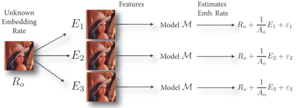
In this paper we propose to use the re-embedding idea to embed again some information inside the considered imageIo. The rationale here is to assume that the reliability of the estimation of the initial embedding rate is function of the reliability after multiple re-embeddings. Multiple such re-embedding with different sizes provide images with a larger embedding rate, of which a part is known. The global idea of the re-embedding and its use in this paper is illustrated in Figure 2.1. Features Estimates Emb. Rate Unknown Embedding Rate Model Model Model
Figure 2: The Re-embedding concept: the original imageIosupposedly hav-ing a payload with embeddhav-ing rateRo is duplicatedN times (N = 3 here) and payloads with number of embedding changes Ei are embedded in it. Features are extracted from each duplicate image (with additional embed-ding changes) and the previously built modelMis used on these features to devise the final embedding rateRi.ˆ
Consider the intercepted imageIo; the idea is to make a known amountEi of new embedding changes toIo. This process is repeatedN times{Ei,1≤ i≤ N}on the imageIo, in order to obtain a set of images{Ii,1≤ i ≤N} for each of whichEi re-embedding changes are performed.
After this re-embedding procedure, the actual embedding rate for image Ii is approximated as Ri = Eo+Ei Ao =Ro+ 1 Ao Ei, (1)
withEo andAo the number of embedding changes and the number of non-zero AC coefficients in the considered imageIo, respectively (the sender of the suspicious imageIohas causedEo embedding changes). It is assumed in this context that the number of non-zero AC coefficientsA might vary due to an embedding. Some stego algorithms attempt to not modify this quantity, though.
In order to illustrate that Eq. 1 is a good approximation for lowEo and Ei, let us introduce two additional notations: the total number of pixels in the imageI, Npix(I)and thereal total number of embedding changesEitot, measured between the original “clean” imageI and the image Ii for which re-embedding withEi embedding changes has been performed.
If the stego algorithmS is assumed to modify directly LSBs of pixels for each embedding change to perform (no matrix encoding, for example), it is possible to estimate the probabilityPpixof a pixel to be modified by both the
first embedding (by the sender) and the re-embedding. Using these notations, it is straightforward, Ppix= Eo Npix(I) × Ei Npix(I) . (2)
Figure 3 illustrates the validity of the approximation made by Eq. 1, for smallEo+Ei (the experiment uses the nsF5 algorithm [15, 7]and Fridrich’s extended DCT calibrated features [5]). Note that the plot of Eo + Ei − Ppix(Eo+Ei) would be barely distinguishable from that of Eo +Ei here,
due to Ppix 1. This is the case when the assumptions on Eo and the range ofEi made in this paper are met: "low" Eo (compared toNpix) and a
controlled small range forEi. In the event of a careless steganographer (Eo exceptionally large) for example, this result might not hold as well as here.
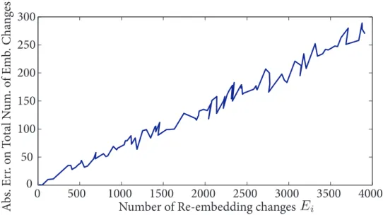
In addition, the absolute error made by the approximation of Eq. 1 ver-sus the number of re-embedding changesEi is depicted on Figure 4 for one image (the behavior is the same for all700images used in this paper). Con-sequently, the largerEi, the more probable it is that some “overlap” happens, between the initial embedding changesEo and the re-embeddingsEi, which is expected from Eq. 2.
The rationale in this paper is that the sender is not careless about the embedding rate used and that the number of re-embedding changes Ei are controlled in a certain range. With these assumptions, Eq. 1 is a reasonable approximation.
Then, in the very same way as that of the quantitative steganalysis, it is pos-sible to obtain an estimation of theRi, using a previously trained regression model M. Denoting Xi = (x1i, . . . , xdi) the d-dimensional feature vector extracted for imageIi, one gets the predicted embedding rateRiˆ =M(Xi).
From Eq. 1 comes
ˆ Ri =Ro+ 1 Ao Ei+εi, (3) 10 2 METHODOLOGY
0 0.5 1 1.5 2 2.5 3 3.5 x 10⁴ 0 0.5 1 1.5 2 2.5 3 3.5 x 10⁴
Real Number of Embedding Changes
Ap pr ox. N um. o f Em b. C ha ng es
Figure 3: Approximated number of total embedding changes by Eq. 1,Eo+ Ei, versus thereal total number of embedding changesEtot. The solid line
denotes the case where (Eo+Ei) = Etot exactly. The plot of Eo +Ei − Ppix(Eo+Ei)is not distinguishable from that ofEo+Ei and is not depicted here. This experiment uses the nsF5 stego algorithm [15, 7].
0 500 1000 1500 2000 2500 3000 3500 4000 0 50 100 150 200 250 300
Number of Re-embedding changes
Abs. Er r. o n T ot al N um. o f Em b. C ha ng es
Figure 4: Absolute Error on the total number of embedding changes abs(Etot−(Eo+Ei))versus the number of re-embedding changesEi.
with εi the error made in the estimation ofRi. It is assumed in the fol-lowing that the εi are independent from each other and from the Ei, for simplicity.
2.2 Confidence interval estimation
Since both quantitiesRˆi andEi are known, the confidence interval and the estimation of the original embedding rateRˆocan then be obtained by solving the linear system
Eo Ao +
1
AoE= ˆR, (4)
withRˆ = ( ˆR1, . . . ,RˆN)T the vector holding the estimations made by model MandE= (E1, . . . , EN)T the vector of the embedding changes performed. This system is solved in a Least Squares sense, by minimizing k εk2, whereε= (ε1, . . . , εN)T, which comes down to the problem
min α,β α+β·E− ˆ R 2 , (5) with α = Eo Ao and β = 1
Ao. This is solved by a classical pseudo-inverse
formulation.
The constant term in the minimization problem is the original rate Ro for which we will obtain “an estimate”Rˆo , along with a confidence interval on the valueRˆo, denotedhRˆINFo ,RˆSUPo i. This confidence interval is obtained using the Matlab® function regress, which uses a Student’s t score, as described in [4]:RˆINFo is obtained by
ˆ RINFo = ˆRo−tα/2,νσˆ ˆ Ro , (6)
wheretα/2,ν is thetscore (inverse Studentt cdf) with parameterα/2(for a
100(1−α)% confidence interval) withνdegrees of freedom (hereν=N−2), andσˆ( ˆRo)is the estimated standard deviation ofRˆo. The upper boundRˆSUPo is computed similarly, and the confidence interval for the first order term also (please refer to [4] for the derivations). One can also obtain the number of non-zero AC coefficientsAowhen solving the system, and hence recover the original number of embedding changesEo.
This is illustrated on a set of images in the experiments section 3.
2.3 Estimation of the inner image difficulty
The inner difficulty of the image can be represented as the variation of the predictions for a given original embedding rateEo when the embedding key, or the embedded message fluctuates (similarly to [2]). Note that this variation is solely due to the characteristics of the cover image. Consequently our rationale is to measure the image difficulty as the standard deviation of the error performed for various embeddings on this image (no re-embeddings).
That is, for a genuine image I, L different embeddings are performed with different number of embedding changes{EO
i ,1 ≤ i ≤ L}. The error εOi between the estimated value of the embedding rate RˆiO (by model M) and the true valueROi is then defined asεO
i =ROi −RˆOi .
The standard deviation of this quantity over theLdifferent realizations is the proposed measure of the inner image difficultyDfor imageI:
DI =std εO , (7) withεO = εO 1, . . . , εOL T .
In order to show that the estimated confidence interval gives information on the inner image difficulty, through the re-embeddings, the quantityDI in-herent to each imageI, is compared to the width of the estimated confidence interval forRo.ˆ
A dependence between the two proves the width of the estimated confi-dence interval can be used as an indicator of the image difficulty measured byDI.
Note that the calculation ofDI for an image requires the use of the gen-uine image, which is not accessible in practice. In the following, theseL embeddings on the cover image are referred to as “original embeddings”.
The following section presents results for this methodology with publicly available algorithms and images.
3 RESULTS
For the following experiments,700images picked at random from the BOWS2 database have been used [1], withL = 100repetitions for the estimation of the image difficultyDI andN = 1500repetitions for the re-embeddings.
For each of the 700 images, initial embedding rates (supposed to be the embedding rate in the intercepted suspicious image) uniformly selected be-tween0and30% are used.
Re-embeddings follow the same range of rates, leading to final embedding ratesRibetween0and about50% for theIi. The stego algorithm used in the experiments is nsF5 [15, 7].
In this paper, the model Mused for the regression is an OP-ELM [10] (the toolbox fromhttp://www.cis.hut.fi/projects/eimlwas used), which is a feedforward neural network using random projections. It has the advan-tage of performing very well (with similar performances to state of the art Ma-chine Learning techniques such as Support Vector MaMa-chines) while keeping a rather low computational time. The OP-ELM optimizes the Mean Square Error. Default parameters (Linear, Sigmoid and Gaussian kernels,300 max-imum number of kernels) have been used for the experiments.
The OP-ELM modelMis used on the274DCT-based features extracted from imageIo [5] augmented by the number of non-zero DCT coefficients of the imageIo.
0 1000 2000 3000 4000 5000 6000 7000 8000 9000 10000 0.2 0.25 0.3 0.35 0.4
Number of Embedding Changes
Es tim at ed Em be ddin g R at e
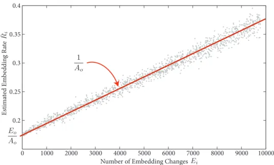
Figure 5: Plot of the estimated embedding rate Rˆi versus the number of embedding changes Ei, for one image. From Eq. 5, the slope gives the β= A1
o term while the value forEi −→0gives theα=
Eo
Ao term.
3.1 Estimation of the original embedding rate Rˆo
First, Figure 5 illustrates the solution of Eq. 5 for one image only (the behav-ior is the same for all images): by solving the linear system in a Least Squares sense, the values ofβ = A1
o (the slope) andα =
Eo
Ao (estimated embedding
rate forEi −→0) are devised. Here, allN = 1500values obtained for each re-embedding are plotted.
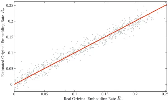
In order to show that the minimization problem is correctly solved for the whole range of embedding rates and for all700images, Figure 6 represents the estimated value of the original embedding rateRˆo versus the real value Ro. The actual Normalized Mean Square Error (NMSE) for the 700 im-ages in this figure using the re-embeddings is0.0330, while using the same model Mdirectly on each image (classical quantitative steganalysis, no re-embedding) leads to a0.0346NMSE in this case.
Hence, using this methodology on the 700 images yields on average an improvement of5% of the NMSE for quantitative steganalysis.
It can be noted that the OP-ELM already performs very well [9] and the nsF5 stego problem is easy enough, hence the difficulty to improve “radi-cally” the performances obtained in the first place.
To investigate the influence of the number of re-embeddingsN, a variable number of re-embeddings has been used to establish Figure 7. It illustrates the evolution of the NMSE using the re-embedding approach, with a varying number of re-embeddingsN. It is interesting to note that the error decreases dramatically with the number of re-embeddings N in the beginning, until the improvement becomes statistically insignificant, beyondN = 1000.
In fact, once there are enough samples (equations) in the system to solve Eq. 4, new re-embeddings (and hence, new equations in the system) do not provide sufficient additional information for the regression problem. Hence
0 0.05 0.1 0.15 0.2 0.25 0 0.05 0.1 0.15 0.2 0.25
Real Original Embedding Rate
Es tim at ed Or ig in al Em be ddin g R at e
Figure 6: Plot of the estimated original embedding RateRoˆ through the re-embeddings versus the originalRo, for all700images.
0 500 1000 1500 0.033 0.034 0.035 0.036 0.037 0.038 0.039 Number of Re-Embeddings N or m alize d MS E
Figure 7: Plot of the Normalized Mean Square Error (NMSE) made onRoˆ versus the number of re-embeddings performed. The solid straight line gives the NMSE using the OP-ELM for classical quantitative steganalysis (no re-embedding), and the straight dashed line the NMSE for an OLS model.
1.5 2 2.5 3 3.5 4 x 10⁻³ 0.005 0.01 0.015 0.02 0.025 0.03
Width of Confidence Interval for
St d o f Er ro r f or fir st Em be ddin gs
Figure 8: Plot ofDI, the standard deviation of the error made on theL “origi-nal embeddings”DI =std εO
versus the width of the estimated confidence intervalRˆSUPo −RˆINFo .
the rather small improvement between1000and1500re-embeddings.
3.2 On the use of the width of the confidence interval
The confidence interval for the experiments has been set to 95% [3], and calculated using the Matlab©regressfunction [4].
Following results make use of the width of the confidence interval on the estimation ofRo. The goal of this experiment is to establish a dependenceˆ between the estimated confidence intervalhRˆIN F
o ,RˆSUPo i
for the embedding rate Roˆ and the inner difficulty DI of the image I considered, in the first place.
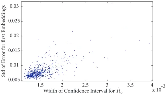
Figure 8 is a graph of the standard deviation of the error made on the “original embeddings”DI =std εO
versusRˆSUPo −RˆINFo .
There appears to be a dependence between the “difficulty” (as estimated by the original embeddings), and the width of the confidence interval esti-mated by the re-embedding approach. Indeed, one can say that the larger is the estimated confidence interval forRo, the larger the probability of theˆ error and therefore the more probable the image is a difficult one.
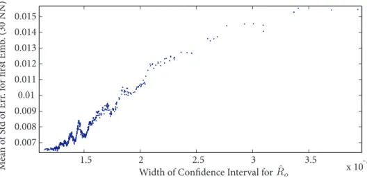
The high correlation between the difficulty and the confidence interval is not very easy to notice on Figure 7 because of the non-uniform distribu-tion of the samples along the abscissa. In order to overcome this visualisadistribu-tion drawback, a local average using the 30 nearest neighbors regarding the x-coordinate is computed, the y x-coordinate being computed by the average of y-coordinates the corresponding points. The result is depicted on Figure 9 where the relation between the estimated confidence interval and the diffi-culty of the images is straightforward.
Figure 9 shows the evolution of this average versus the width of the esti-mated confidence interval. In fact, if one considers the cloud of points of
1.5 2 2.5 3 3.5 x 10⁻³ 0.007 0.008 0.009 0.01 0.011 0.012 0.013 0.014 0.015
Width of Confidence Interval for
M ea n o f S td o f Er r. f or fir st Em b. (30 NN)
Figure 9: Plot of the mean ofDI for the 30 nearest neighbors (with respect toDI) versus the width of the estimated confidence interval.
1.5 2 2.5 3 3.5 4 x 10⁻³ 0 0.5 1 1.5 2 2.5 3 3.5 4 4.5x 10⁻⁵
Width of Confidence Interval for
Va r. o f S td . o f Er r. o n fir st Em b. (30 NN)
Figure 10: Plot of the variance ofDI for the 30 nearest neighbors (with re-spect toDI) versus the width of the estimated confidence interval.
Figure 8 as a “flat cone”, Figure 9 plots the evolution of the center of the cone. It is then obvious that the larger the estimated confidence interval, the more difficult is the image to handle in steganalysis, in terms of the criterion DI (inner difficulty).
Finally, Figure 10 shows the evolution of the variance of DI for the 30 nearest neighbors for each image. The growth shows that the larger the con-fidence interval, the more difficult it is to have an accurate estimation of the difficulty. From Figures 9 and 10, we can conclude that the probability to get a largeDIis increasing with respect to the width of the calculated confidence interval.
4 CONCLUSION
In this paper, an approach based on multiple re-embeddings is used to esti-mate in terms of quantitative steganalysis, the original embedding rate (and the number of embedding changes) in an intercepted image. The proposed methodology makes it possible to obtain a reliable estimation of this embed-ding rate — with a small improvement in terms of accuracy —, along with a confidence interval on this value.
The estimated confidence interval in turn enables the steganalyzer to mea-sure the inherent difficulty of the image (reliability estimation), in terms of classical quantitative steganalysis. Through the width of this confidence in-terval, it becomes possible to rank the images of a database in terms of their probability of difficulty for quantitative steganalysis, without possessing the genuine images nor having any information on their being stego or genuine. The proposed methodology has the advantage of being usable for any stego algorithm (given the assumptions made in section 2) and any regres-sion model. Future work will apply this methodology to other stego algo-rithms (MMX, JPHS, Outguess, StegHide. . . ), a larger image database and other regression models, such as SVR. Also, an analysis of the error εi (in its relation to the embedding changesEiand on the assumed independence between theεi) could lead to a better modelisation and a more accurate esti-mation of the embedding rate and hence of inner image difficulty.
ACKNOWLEDGMENTS
The authors would like to thank Tomáš Pevný for his advices on addressing on the Quantitative Steganalysis problem.
REFERENCES
[1] Patrick Bas and Teddy Furon. BOWS2 challenge: Break our water-marking scheme. ECRYPT European Network of Excellence, http: //bows2.gipsa-lab.inpg.fr/.
[2] Rainer Böhme and Andrew D. Ker. A two-factor error model for quan-titative steganalysis. In Edward J. Delp III and Ping Wah Wong, editors,
Proceedings of SPIE, volume 6072, page 607206. SPIE, 2006.
[3] Samprit Chatterjee and Ali S. Hadi. Influential observations, high leverage points, and outliers in linear regression. Statistical Science, 1(3):379–393, 1986.
[4] Norman R. Draper and Harry Smith. Applied Regression Analysis, 3rd edition. Wiley-Interscience, 1998.
[5] Jessica Fridrich. Feature-based steganalysis for jpeg images and its im-plications for future design of steganographic schemes. InInformation Hiding: 6th International Workshop, volume 3200 ofLecture Notes in Computer Science, pages 67–81, May 23-25 2004.
[6] Jessica Fridrich, Miroslav Goljan, Dorin Hogea, and David Soukal. Quantitative steganalysis of digital images: estimating the secret mes-sage length. Multimedia systems, 9(3):288–302, 2003.
[7] Jessica Fridrich, Tomáš Pevný, and Jan Kodovský. Statistically unde-tectable jpeg steganography: dead ends challenges, and opportunities. In MM&Sec ’07: Proceedings of the 9th workshop on Multimedia & security, pages 3–14, New York, NY, USA, 2007. ACM.
[8] Auguste Kerckhoffs. La cryptographie militaire. Journal des sciences militaires, 9:5–38, January 1883.
[9] Yoan Miche, Patrick Bas, Amaury Lendasse, Christian Jutten, and Olli Simula. Reliable steganalysis using a minimum set of samples and features. EURASIP Journal on Informa-tion Security, 2009(1):1–13 (Article ID 901381), March 2009. http://www.hindawi.com/journals/is/2009/901381.html.
[10] Yoan Miche, Antti Sorjamaa, Patrick Bas, Olli Simula, Christian Jutten, and Aamaury Lendasse. OP-ELM: Optimally-pruned extreme learning machine. IEEE Transactions on Neural Networks, 21(1):158–162, Jan-uary 2010.
[11] Tomáš Pevný and Jessica Fridrich. Towards multi-class blind stegan-alyzer for jpeg images. In International Workshop on Digital Water-marking 2005, volume 3710 ofLNCS, pages 39–53, 2005.
[12] Tomáš Pevný and Jessica Fridrich. Multiclass blind steganalysis for jpeg images. InSPIE Electronic Imaging, volume 6072, page 60720O, 16-19 January 2006.
[13] Tomáš Pevný, Jessica Fridrich, and Andrew D. Ker. From blind to quan-titative steganalysis. In Edward J. Delp III, Jana Dittmann, Nasir D. Memon, and Ping Wah Wong, editors, Media Forensics and Security, volume 7254, page 72540C. SPIE, 2009.
[14] Hedieh Sajedi and Mansour Jamzad. Secure steganography based on embedding capacity. International Journal of Information Security, 8(6), December 2009.
[15] Andreas Westfeld. F5-a steganographic algorithm. In IHW ’01: Pro-ceedings of the 4th International Workshop on Information Hiding, pages 289–302, London, UK, 2001. Springer-Verlag.
TKK REPORTS IN INFORMATION AND COMPUTER SCIENCE
TKK-ICS-R24 Timo Honkela, Nina Janasik, Krista Lagus, Tiina Lindh-Knuutila, Mika Pantzar, Juha Raitio Modeling communities of experts. December 2009.
TKK-ICS-R25 Jani Lampinen, Sami Liedes, Kari Ka¨hko¨nen, Janne Kauttio, Keijo Heljanko Interface Specification Methods for Software Components. December 2009.
TKK-ICS-R26 Kari Ka¨hko¨nen
Automated Test Generation for Software Components. December 2009.
TKK-ICS-R27 Antti Ajanki, Mark Billinghurst, Melih Kandemir, Samuel Kaski, Markus Koskela, Mikko Kurimo, Jorma Laaksonen, Kai Puolama¨ki, Timo Tossavainen
Ubiquitous Contextual Information Access with Proactive Retrieval and Augmentation. December 2009.
TKK-ICS-R28 Juho Frits
Model Checking Embedded Control Software. March 2010.
TKK-ICS-R29 Miki Sirola, Jaakko Talonen, Jukka Parviainen, Golan Lampi
Decision Support with Data-Analysis Methods in a Nuclear Power Plant. March 2010.
TKK-ICS-R30 Teuvo Kohonen
Contextually Self-Organized Maps of Chinese Words. April 2010.
TKK-ICS-R31 Jefrey Lijffijt, Panagiotis Papapetrou, Niko Vuokko, Kai Puolama¨ki
The smallest set of constraints that explains the data: a randomization approach. May 2010.
TKK-ICS-R32 Tero Laitinen
Extending SAT Solver With Parity Constraints. June 2010.
TKK-ICS-R33 Antti Sorjamaa, Amaury Lendasse
Fast Missing Value Imputation using Ensemble of SOMs. June 2010.
ISBN 978-952-60-3249-8 (Print) ISBN 978-952-60-3250-4 (Online) ISSN 1797-5034 (Print)