The Breakdown Behavior of the Maximum Likelihood
Estimator in the Logistic Regression Model
Christophe Croux
∗C´
ecile Flandre
†Gentiane Haesbroeck
‡Abstract: In this note we discuss the breakdown behavior of the Maximum Likelihood (ML) estimator in the logistic regression model. We formally prove that the ML-estimator never explodes to inÞnity, but rather breaks down to zero when adding severe outliers to a data set. An example conÞrms this behavior.
Keywords: Breakdown Point, Logistic Regression, Maximum Likelihood, Robust Estimation.
AMS subject classification: 62F35, 62G35.
∗Dept. of Applied Economics, Katholieke Universiteit Leuven, Naamsestraat 69, B-3000 Leuven, Belgium,
Email: [email protected].
†Cardif Vie S.A., Chauss´ee de la Hulpe 150, B-1170 Bruxelles, Belgium, Email: [email protected]. ‡Dept. of Mathematics, University of Li`ege (B37), Grande Traverse 12, B-4000 Li`ege, Belgium, Email:
1
Introduction
One aim in robust statistics is to build high breakdown point estimators. The breakdown point of an estimator tells us which percentage of the data may be corrupted before the esti-mator becomes completely unreliable. In linear regression models, the breakdown points of many robust estimators have been calculated. Robust estimators have also been introduced for the logistic regression model, but their breakdown points are not well established. In fact, even the study of the breakdown behavior of the classical Maximum Likelihood estimator has not been completed yet.
Christmann (1994) showed that any sensible estimator in the logistic model, robust or not, will tend to inÞnity if one replaces a certain number of observations to well chosen positions. The replacement breakdown point of Donoho and Huber (1983) seems therefore not to be appropriate for measuring robustness of estimators in logistic regression1. This has also been noticed by K¨unsch, Stefanski and Carroll (1989, section 4) who therefore proposed to investigate what happens when outliers are added to a sample.
First, we prove in Section 2 that the classical Maximum Likelihood estimator (ML) stays uniformly bounded if one adds outliers to the original sample. On the other hand, it is shown in Section 3 that the norm of the ML-estimator always tends to zero, when adding only a few badly placed outlying observations. These results motivated a new deÞnition of the Þnite sample breakdown point for an estimator in the logistic regression model. In Section 4, an example illustrates the breakdown behavior of the classical estimator.
1An exception is the logistic regression model with large strata where replacement breakdown points can
2
Explosion Robustness of the ML-Estimator
Let z∗
i = (xti, yi∗)t∈ IR p−1
×IR (i = 1, . . . , n) be realizations of independent p-dimensional random vectors Z∗
i = (Xit, Yi∗)t, following the model
Yi∗ =α+Xitβ+εi (2.1)
where εi follows a symmetric distribution with a strictly increasing cumulative distribution
function F. Taking F(u) = 1/(1 + exp(−u)) results in the logit model, while the probit is obtained using the normal cumulative distribution function for F. Typically, in the logistic model with binary data, the underlying dependent variable Y∗ is non observable, and only
the dummy variable Y obtained by taking
yi = 0 if y∗ i ≤0 1 if y∗i >0 (2.2)
can be recorded. Therefore, we get P(Yi =yi |Xi =xi) =F(α+xtiβ)
yin1
−F(α+xtiβ)o1−yi for yi = 0,1. (2.3)
In what follows,Zn ={z1, . . . , zn}denotes the observed sample, and we will use the notations
γ = (α,βt)t and ˜x
i = (1, xit)t for all 1 ≤ i ≤ n. An estimator for γ computed from the
sample Zn is denoted by ˆγ(Zn) or simply ˆγn. The ML-estimator ˆγnM L is deÞned as
ˆ γnM L= argmax γ logL(γ;Zn) = argminγ n X i=1 d(γ;zi)
where logL(γ;Zn) is the log-likelihood function calculated inγandd(γ;zi) =−yilogF(˜xtiγ)−
(1−yi) log{1−F(˜xtiγ)} stands for the deviance at observation i.
We will assume throughout the paper the existence of the ML-estimator at the observed sample, yielding a Þnite kˆγM L
n k, wherek.kdenotes the Euclidean norm. The latter condition
leads to the overlap situation described by Albert and Anderson (1984) and Santner and Duffy (1986), excluding complete or quasi-complete separation between the observations
with yi = 0 and yi = 1. This means that if we denote I1 = {i∈{1, ..., n}|yi = 1} and its
complement I0 ={i∈{1, ..., n}|yi = 0}, we cannot Þnd any γ ∈IRp such that
˜
xtiγ ≥0 ∀i∈I1 and x˜tiγ ≤0 ∀i∈I0. (2.4) In particular, this condition excludes the situation where all yi are equal.
To study the robustness of estimators, we will introduce data contamination by adding m potential outliers to the original data set Zn. These added observations zi = (xti, yi)t
may have completely arbitrary values for the explicative variables, meaning that we allow for leverage points in the contaminated sample. The yi values are of course restricted to
be one or zero, otherwise they are immediately identiÞable as typing errors. In the fol-lowing, ˆγ(Z0
n+m) denotes the estimator computed from the contaminated sample Zn0+m =
{z1, ..., zn, zn+1, ..., zn+m}. The explosion breakdown point ε+(ˆγn;Zn) of the estimator ˆγn at
the sample Zn is then deÞned as the minimal fraction of outliers that need to be added to
the original sample before the estimator tends to inÞnity:
ε+(ˆγn;Zn) =m+/(n+m+) withm+= min{m| sup zn+1,...,zn+mk
ˆ
γ(Zn0+m)k=∞}.
(If the set over which we take the minimum is empty, then we set ε+(ˆγ
n;Zn) = 1.)
If we add outliers to Zn, then the contaminated data set Zn0+m remains in the overlap
situation, so every ˆγ(Zn0+m) remainsÞnite. The next Theorem shows that the ML-estimator
even remains uniformly bounded (i.e. the bound remains the same for all possible conÞ gu-rations of contamination) when adding outliers. The proof is given in the Appendix.
Theorem 1. Suppose that kˆγM L(Z
n)k < ∞. For every finite number m of outliers, there
exists a real positive constant M(Zn, m) such that
sup
zn+1,...,zn+m k
ˆ
γM L(Zn0+m)k≤M(Zn, m).
As a corrolary we have ε+(ˆγM L
n ;Zn) = 1.We will call this property the explosion robustness
classical estimator in linear regression, which can become arbitrarily large just by adding one single outlier. Note also that Theorem 1 contradicts the assertion of K¨unsch et al (1989, Section 4), who claimed that ML-estimator could tend to inÞnity when extreme outliers are added.
Instead of adding outliers, one could also think of replacing good observations by con-taminants. Christmann (1994) showed that the minimal number of observations that need to be replaced before the estimator tends to inÞnity equals the number of observations in “overlap.” This number depends only on the sample and is the same for every sensible estimator. The effect of replacing good observations by outliers is quite different from the impact of adding outliers, which distinguishes the logistic regression model from the usual linear regression model. In the next section we will motivate a new deÞnition of breakdown point for the logistic regression model.
3
Breakdown Point in Logistic Regression
We will focus on the slope parameterβ. This parameter can be written asβ = kββkkβk=θ/σ
withkθk= 1 andσ= 1/kβk.We interpret the vectorθ as the direction in which we move the “fastest” from the observations in I0 to these from I1, whereas σ measures this “fastness”.
Since the parameter θ belongs to Sp−2 = nθ
∈IRp−1| kθk= 1o which has no border, an estimator of θ never breaks down. On the contrary, the parameter σ belongs to [0,+∞], including two types of possible breakdown for an estimator ˆσn. We will say that an estimator
ˆ
σn of σ implodes if it tends to 0 and explodes if it becomes inÞnite. This corresponds to an
explosion of ˆβn, respectively an implosion of (the norm of) ˆβn. A discussion of these two
extremal cases is presented below.
Case 1: If ˆβn explodes, then only the sign of ˜xtiγˆn matters. The Þtted probabilities will
all be zero or one. We can therefore say, as in Stromberg and Ruppert (1992), that theÞtted values break down.
Case2: If kβˆnk decreases to 0, the error term in (2.1) dominates. Explanatory variables
have then no inßuence on the dummy variableyi, so the model becomes obviously senseless.
The Þtted probabilities are all equal.
The addition breakdown point of ˆβn is now deÞned as the smallest proportion of
conta-mination that can cause the estimator to grow to inÞnity or to vanish into zero.
Definition 1. The breakdown point of an estimatorβˆnfor the logistic regression model (2.3)
at the sample Zn is given by ε∗( ˆβn;Zn) =m∗/(n+m∗) with m∗ = min(m+, m−),
m+ = min{m∈IN0| sup zn+1,...,zn+mk ˆ β(Zn0+m)k=∞} m− = min{m∈IN0|z inf n+1,...,zn+mk ˆ β(Zn0+m)k= 0},
where Zn0+m is obtained by adding m arbitrary points to Zn.
In the previous section it was shown that the ML-estimator never explodes, but the next theorem shows that it is always possible to Þnd 2(p−1) outliers such that the ML slope estimator tends to zero while adding these well chosen points (The proof can be found in the Appendix).
Theorem 2. At any sample Zn, the breakdown point of the ML-estimator satisfies
ε∗( ˆβM L;Zn)≤
2(p−1) n+ 2(p−1).
It follows that the asymptotic breakdown point limnε∗( ˆβM L;Zn) equals zero. The above
theorem formally shows the non robustness of the ML-estimator. Not because it explodes to inÞnity (as is often believed), but because it can implode to zero when adding outliers to the data set. It can be checked that the standard errors of the ML-estimator explode together with the estimator, but this is not true for implosion to zero. The latter type of breakdown is therefore harder to detect. The most dangerous outliers, as can be seen from the proof of Theorem 2, are misclassiÞed observations (meaning that ˆαn+xtiβˆn and yi have different
them bad leverage points. These inßuential points were already pointed out by Stefanski et al. (1986) who proposed estimators downweighting them.
It might be a bit strange to speak of breakdown when the estimator tends to a central point in the parameter space. A similar phenomenom is seen in the autoregressive model of order one, where the Least Squares estimator is driven to zero in presence of badly placed outliers. This example motivated Genton and Lucas (2000) to introduce a very general notion of breakdown point, which depends on the type of outlier constellation one considers and on a certain badness measure (measuring how bad an estimated parameterÞts the data). When applying their deÞnition to the logistic regression model, using bad leverage points as outlier constellation and the sum of deviances as badness measure, we obtain an expression equivalent to the implosion breakdown point considered above.
Remark: Theorem 1 implies that the intercept estimator is explosion robust. On the other hand if the slope estimator tends to zero, ˆαM Ln will return F−1(ˆpn+m), where 0<pˆn+m <1
is the frequency of observations in Zn0+m with yi = 1, which will in general be different from
0.
4
Example and Conclusion
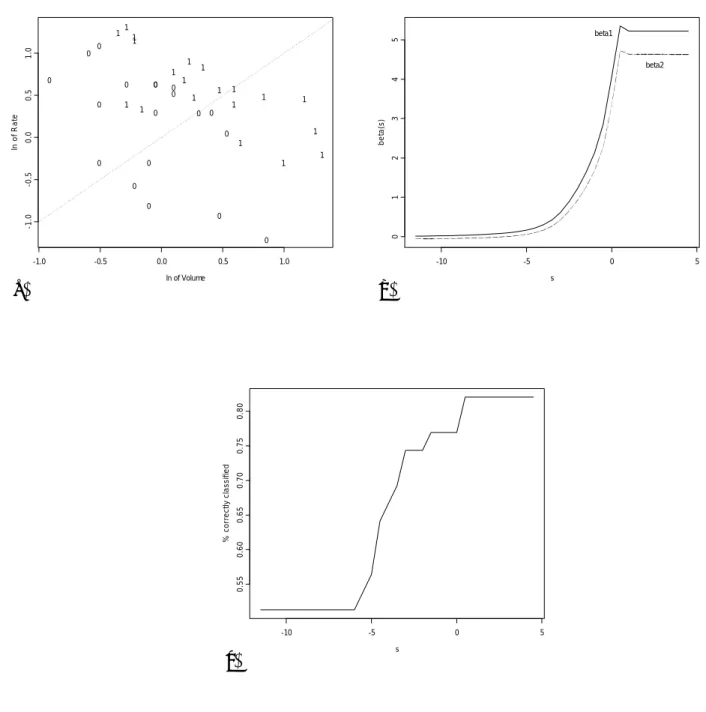
Consider the well-known Vaso Constriction data set of Finney (1947), see also Pregibon (1982). The binary outcomes (presence or absence of vaso-constriction of the skin of the digits after air inspiration) are explained by two explanatory variables: x1 the volume of
air inspired and x2 the inspiration rate (both in logarithms). Figure 1a gives the scatter
plot of these data in the covariate space, together with the y-value. To assess the effect of contamination on the ML estimator, we added one outlier with (x1, x2, y) = (s, s,1) to the
n = 39 observations of the sample, and computed an estimator ˆβ(s) based on these 40 data points. By letting s move along the real line, the outlier follows the dotted line of Figure 1a. We see from the Þgure that for large values of s the added observation will be correctly
classiÞed and will therefore be a good leverage point. For large negative values of s we get a bad leverage point.
To visualize the inßuence of the contaminant (s, s,1) on the estimates, we plotted the values of ˆβ(s) with respect to s in Figure 1b. Since ˆβML
n = (5.220,4.631), we see that good
leverage points do not perturb the Þt obtained by the ML procedure (reason why we call them “good”). On the other hand, for s tending to −∞, a bad leverage point breaks the slope estimator towards zero. If we look at the robustness in terms of the percentage of correctly classiÞed observations (Figure 1c), we see that, in presence of a bad leverage point, the percentage of well classiÞed observations gets close to 50%, which is the same success rate as a random classiÞcation rule can attain.
The above example illustrates the non-robustness of the ML estimators. Since Pregibon (1982), many authors have proposed robust procedures for this model, e.g. Copas (1988), K¨unsch et al. (1989), Morgenthaler (1992), Carroll and Pederson (1993), Bianco and Yohai (1996). The breakdown points of these estimators have not been derived yet, but it seems to be a difficult task and their values will depend heavily on the sample.
Acknowledgment: We wish to thank Andreas Christmann for very helpful remarks.
Appendix
Proof of Theorem 1: For every γ, deÞne δ(γ, Zn) = inf n ρ>0| ∃i∈I1 such that ˜xtiγ <−ρ or∃i∈I 0 such that ˜xtiγ >ρ o . Due to (2.4), 0 < δ(γ, Zn) < +∞. Indeed, if δ(γ, Zn) is not Þnite we would have ˜xtiγ ≥ 0∀i ∈ I1 and ˜xt
iγ ≤ 0 ∀i ∈ I0, which contradicts the overlap supposition. Consider the
compact set Sp−1 =
in γ, we have
δ∗(Zn) = inf
γ∈Sp−1 δ(γ, Zn)>0.
Denote ˆγn+m the ML-estimator in the logistic regression based on a contaminated sample
Z0
n+m where arbitrary points zn+1, . . . , zn+m have been added. Since ˆγn+m minimizes the
sum of the deviances d(γ;zi) of the sample points, we set
D(ˆγn+m;Zn0+m) := minγ nX+m
i=1
d(γ;zi).
Putting D0 the total deviance for γ = 0, and using symmetry of F, we have that
D0 :=D(0, Zn0+m) = nX+m
i=1
d(0;zi) = (n+m) log 2.
Take ˜z = exp(−D0) and deÞne
M(Zn, m) =
F−1(1−z)˜
δ∗(Zn) , (4.1)
which is a constant only depending on the original sample Zn and on the number m of
observations added to Zn. Suppose now that ˆγn+m satisÞes
kγˆn+mk> M(Zn, m). (4.2)
First of all, for each ˆγn+m ∈IRp, we know that there exists at least one 1≤i0 ≤n such that
i0 ∈I0 and ˜xti0 ˆ γn+m kˆγn+mk ≥ δ à ˆ γn+m kγˆn+mk , Zn ! ≥δ∗(Zn)>0. (4.3) or i0 ∈I1 and ˜xti0 ˆ γn+m kˆγn+mk ≤ − δ à ˆ γn+m kγˆn+mk , Zn ! ≤ −δ∗(Zn)<0. (4.4)
These two cases have to be studied separately:
Case1: For i0 verifying (4.3), it follows from (4.1) and (4.2) that
D(ˆγn+m;Zn0+m) = nX+m
i=1
d(ˆγn+m, zi)
= −log " 1−F à kγˆn+mkx˜ti0 ˆ γn+m kˆγn+mk !# ≥ −log [1−F (kγˆn+mkδ∗(Zn))] > −log [1−F (M(Zn, m)δ∗(Zn))] = −log(˜z) =D0.
Case2: For i0 satisfying (4.4), we obtain in a similar way
D(ˆγn+m, Zn0+m) = nX+m i=1 d(ˆγn+m, zi) ≥ d(ˆγn+m, zi0) = −log " F à kγˆn+mkx˜ti0 ˆ γn+m kγˆn+mk !# = −log " 1−F à −kˆγn+mkx˜ti0 ˆ γn+m kγˆn+mk !# ≥ −log [1−F (kγˆn+mkδ∗(Zn))] > −log [1−F (M(Zn, m)δ∗(Zn))] = −log(˜z) =D0.
We conclude that D(ˆγn+m, Zn0+m) > D0 = D(0, Zn0+m) implying that ˆγn+m cannot be the
ML-estimator. Therefore, equation (4.2) does not hold which proves the theorem. 2
Proof of Theorem 2:
Let δ > 0 be Þxed and denote Zn = {(1, xi, yi)|1≤ i≤n} the observed sample. It is
always possible to Þnd a positive constant ξ such that −logF(−ξ) = D0 = (n+m) log 2.
Furthermore, set M = max1≤i≤nkxik, N = ξδ, A = (p−1) 1
2(2N +M) and m = 2(p−1).
Take {e1, . . . , ep−1} the canonical basis ofIRp−1 and add the set of m outliers
n
zi0 = (1, vi,0), z1i = (1, vi,1), with vi =Aei, for i= 1, . . . , p−1 o
to Zn. We will prove that for all β with kβk>δ and every α
D³(α,β), Zn0+m´> D0 =D
³
yielding that the ML-estimator veriÞes
kβˆnM L+mk<δ. (4.6)
Since (4.6) will hold for every δ > 0, we have proven the theorem, since it implies that we can make kβˆML
n+mk arbitrary small by addingm= 2(p−1) outliers.
In order to prove (4.5), takekβk>δandα arbitrarily, and deÞne the (p−2) dimensional hyperplane Hδ = nx∈IRp−1;α+xtβ = 0o. The Euclidean distance between a vector x
∈
IRp−1 andHδequals dist(x, Hδ) =¯¯¯xt β
kβk +
α
kβk
¯ ¯
¯. First, suppose that there exists an 1≤i0 ≤
p−1 such thatdist(vi0, Hδ)> N. Ifβ tv
i0+α>0, consider the outlierz
0 i0. We obtain readily that βtv i0 +α> Nkβk> Nδ =ξ and d³(α,β), zi00´ = −log³1−F(βtvi0 +α) ´ > −log (1−F(ξ)) = −logF(−ξ) =D0. (4.7)
For βtvi0 +α <0, the outlier z
1 i0 will verify d³(α,β), z1i0´ = −log³F(βtvi0 +α) ´ > −logF(−ξ) =D0 (4.8) since −(βtvi0 +α)>ξ.
On the other hand, suppose that dist(vj, Hδ) ≤N for all 1 ≤j ≤p−1. Denote j0 the
index such that |βj0| = max1≤j≤p−1|βj|. We have (p−1) 1 2|βj
0| ≥ kβk. First suppose that βj0 >0. Then, dist(vj0, Hδ) = |βtvj0 +α| kβk = |α+βj0A| kβk ≤N,
yielding α≤Nkβk−βj0A and therefore
−α≥βj0A−Nkβk≥ Ã A (p−1)12 − N ! kβk= (M +N)kβk.
Take now an observation zi0 from Zn with yi0 = 1. Then we obtain
α+βtxi0 ≤α+kxi0kkβk≤ −(M+N)kβk+Mkβk=−Nkβk<−Nδ=−ξ.
The latter inequality implies as above that
d((α,β), zi0) = −log ³
F(α+βtxi0) ´
> −logF(−ξ) =D0. (4.9)
For βj0 < 0, we can prove in a similar way that there exists an observation zi0 satisfying
d((α,β), zi0)> D0.
From (4.7), (4.8), and (4.9), we conclude that we can alwaysÞnd an observation inZn0+m
which contributes at least D0 to the total deviance. This proves (4.5) and ends the proof. 2
5
References
Albert, A., and Anderson, J.A. (1984). On the Existence of Maximum Likelihood Estimates in Logistic Regression Models,Biometrika, 71, 1—10.
Bianco, A. M., and Yohai, V. J. (1996). Robust Estimation in the Logistic Regression Model, in Robust Statistics, Data Analysis, and Computer Intensive Methods, 17—34;
Lecture Notes in Statistics109, Springer Verlag, Ed. H. Rieder. New York.
Carroll, R. J., and Pederson, S. (1993). On Robust Estimation in the Logistic Regression Model,Journal of the Royal Statistical Society B, 55, 693—706.
Christmann, A. (1994). Least Median of Weighted Squares in Logistic Regression with Large Strata,Biometrika, 81, 413—417.
Copas, J.B. (1988). Binary Regression Models for Contaminated Data, Journal of the Royal Statistical Society B,50, 225—265.
Donoho, D.L., and Huber, P.J. (1983). The notion of breakdown point. In A Festschrift for Erich Lehmann, P. Bickel, K. Doksum, and J.L. Hodges, eds. Wadsworth, Belmont, CA.
Finney, D.J. (1947). The estimation from individual records of the relationship between dose and quantal response. Biometrika, 34, 320—334.
Genton, M.G., and Lucas, A. (2000). Comprehensive DeÞnitions of Breakdown Points for Independent and Dependent Observations. Tinbergen Institute, Discussion paper TI 2000-40/2. Under Revision for publication.
K¨unsch, H.R., Stefanski, L.A., and Carroll, R.J. (1989). Conditionally Unbiased Bounded Inßuence Estimation in General Regression Models, with Applications to Generalized Linear Models,Journal of the American Statistical Association, 84, 460—466.
Morgenthaler, S. (1992). Least Absolute Deviations Þts for generalized linear models. Bio-metrika,79, 747—754.
M¨uller, C.H., and Neykov, N. (2001). Breakdown points of trimmed likelihood estimators and related estimators in generalized linear models. To appear in theJournal of Statistical Planning and Inference.
Pregibon, D. (1982). Resistant Fits for some commonly used Logistic Models with Medical Applications,Biometrics, 38, 485—498.
Santner, T. J., and Duffy, D.E. (1986). A note on A. Albert and J.A. Anderson’s Conditions for the Existence of Maximum Likelihood Estimates in Logistic Regression, Biometrika,
73, 755—758.
Stefanski, L.A., Carroll, R.J., and Ruppert, D. (1986). Optimally bounded score functions for generalized linear models with applications to logistic regression,Biometrika,73, 413— 424.
Stromberg, A., and Ruppert, D. (1992). Breakdown in nonlinear regression, Journal of the American Statistical Association,87, 991—997.
(a) -1.0 -0.5 0.0 0.5 1.0 -1 .0 -0 .5 0 .0 0 .5 1 .0 1 1 1 1 1 1 0 0 0 0 0 0 0 1 1 1 1 1 0 1 0 0 0 0 1 0 1 0 1 0 1 0 0 1 1 1 0 0 1 ln of Volume ln o f R a te (b) s be ta (s ) -10 -5 0 5 0123 4 5 beta1 beta2 (c) s % co rr e c tl y cl a ssi fi e d -10 -5 0 5 0. 55 0. 60 0 .65 0 .70 0. 75 0. 80
Figure 1: Stability experiment for the “Vaso Constriction” data : (a) Scatterplot of the observations (x1i, x2i), indicated by their yi value. (b) Estimates of the slope parameters,
(c) % of correctly classiÞed observations, when adding (s, s,1) to the data set, as a function of s.