University of Arkansas, Fayetteville
ScholarWorks@UARK
Theses and Dissertations
12-2014
Online Detection of Outliers and Structural Breaks
using Sequential Monte Carlo Methods
Richard Wanjohi
University of Arkansas, Fayetteville
Follow this and additional works at:http://scholarworks.uark.edu/etd
Part of theLongitudinal Data Analysis and Time Series Commons
This Dissertation is brought to you for free and open access by ScholarWorks@UARK. It has been accepted for inclusion in Theses and Dissertations by an authorized administrator of ScholarWorks@UARK. For more information, please [email protected], [email protected].
Recommended Citation
Wanjohi, Richard, "Online Detection of Outliers and Structural Breaks using Sequential Monte Carlo Methods" (2014).Theses and
Dissertations. 2076.
Online Detection of Outliers and Structural Breaks using Sequential Monte Carlo Methods
Online Detection of Outliers and Structural Breaks using Sequential Monte Carlo Methods
A dissertation submitted in partial fulfilment of the requirements for the degree of Doctor of Philosophy in Mathematics
by
Richard Wanjohi Kenyatta University
Bachelor of Education (Science), 2007 University of Arkansas
Master of Science in Statistics, 2009
December 2014 University of Arkansas
This dissertation is approved for recommendation to the Graduate Council.
Dr. Giovanni Petris Dissertation Director Dr. Edward Gbur Committee Member Dr. Avishek Chakraborty Committee Member Dr. Mark Arnold Committee Member
Abstract
Outliers and structural breaks occur quite frequently in time series data. Whereas outliers often contain valuable information about the process under study, they are known to have serious negative impact on statistical data analysis. Most obvious effect is model
misspecification and biased parameter estimation which results in wrong conclusions and inaccurate predictions. Structural time series consist of underlying features such as level, slope, cycles or seasonal components. Structural breaks are permanent disruptions of one or more of these components and might be a signal of serious changes in the observed process. Detecting outliers and estimating the location of structural breaks has progressively
become monumental both as a theoretical research problem and an essential part of applied data analysis. Among numerous applications include finance, industrial manufacturing, medical informatics, severe weather prediction. Given that these data arrive rather frequently and sequentially in time, fast reliable and accurate detection techniques are required. We propose a model from class of state-space models of the form yt =f(Xt, ψ, vt)
and Xt=g(Xt−1, ψ, wt) where
Xt t≥0 is a hidden Markov state process. The inference of
Xt t≥0 depends on the observation process {yt}t≥1 and the parameter vector ψ, whose
elements are usually unknown. The innovations vt and wt are conditionally Gaussian given
the precision parameterλ and auxiliary state ω. We employ sequential Monte Carlo techniques to approximate the joint target distributionp(X0:t, ψ|y1:t). The posterior
estimates for the auxiliary statesω will be used to identify outliers and structural breaks. The results prove that the algorithm is comparable to traditional and computationally expensive MCMC and superior to regular techniques such as Exponentially Weighted Moving Average (EWMA), Shewhart, and cumulative sum (CUSUM) control charts
Acknowledgements
I would like to thank my advisor Dr. Giovanni Petris for his patience, support, and
encouragement throughout my time at University of Arkansas. His guidance has made this a thoughtful and rewarding journey.
I would like to thank my dissertation committee for all their support and much needed insights. I also like to thank the department of Mathematical Sciences for granting me graduate assistantship, throughout my study, without which it would have been very difficult to realise my goal.
I would like to thank most sincerely my wife Lydia, sons Henry and Alan for their unconditional love, patience and support throughout the course.
Finally, I would like to thank all my family members and friends for their prayers and for expecting nothing less than completion from me.
Contents
Abstract
Acknowledgements
List of Figures
List of Abbreviations and Symbols
1 Introduction 1
2 Outliers and Structural breaks: Review 9
2.1 Statistical Process Control (SPC) . . . 13
2.1.1 Quality Control Charts . . . 13
2.1.2 Shewhart charts . . . 14
2.1.3 Cumulative Sum (CUSUM) charts . . . 14
2.1.4 Exponentially Weighted Moving Average (EWMA) . . . 18
2.2 ARMA and GARCH models . . . 19
2.3 Regression models . . . 22
2.3.1 Hat Matrix . . . 24
2.3.2 Cook’s Distance . . . 24
2.3.3 DFFITS . . . 24
2.3.4 DFBETAS . . . 25
2.4.1 Static data . . . 25
2.4.2 Time series data . . . 26
3 State Space Model 28 3.1 General State Space Model . . . 28
3.2 Dynamic Linear Model (DLM) . . . 31
3.2.1 Structural Time Series . . . 33
3.2.2 ARMA representation . . . 34
3.2.3 Kalman Filter . . . 35
3.2.4 Forward Filtering Backward sampling (FFBS) . . . 36
3.2.5 MCMC in DLM . . . 37
4 Sequential Monte Carlo (SMC) Methods 38 4.1 Importance sampling . . . 39
4.2 Resampling and auxiliary index . . . 41
4.3 Convergence results . . . 43
4.4 Particle Filters . . . 44
4.4.1 Bootstrap Filter (BF) . . . 44
4.4.2 Auxiliary Particle Filter (APF) . . . 45
4.4.3 The Auxiliary Particle filter with parameter estimation . . . 45
4.4.4 Particle filtering and learning using sufficient statistics . . . 46
5 Model for structural breaks and Outliers 48 5.1 Fat-tailed t-distribtution & Mixture of Normals . . . 48
5.2 Prior specifications . . . 50
5.3 Parameter Estimation . . . 51
5.3.1 Kernel Mixture approximation . . . 51
5.3.2 MCMC moves . . . 52
5.3.4 Hybrid of Kernel approximation and sufficient statistics approaches . 53
5.4 State Estimation . . . 56
5.4.1 Sequential Bridge Sampling . . . 57
5.4.2 Scoring the data . . . 59
5.5 Algorithm Summary . . . 60
6 Application and Results 63 6.1 Nile River problem . . . 63
6.2 Simulated data . . . 66
6.2.1 Local level model . . . 66
6.2.2 Linear trend model . . . 72
6.3 An outlier or structural break? . . . 75
6.3.1 Scenario 1 . . . 75
6.3.2 Scenario 2 . . . 77
6.3.3 Scenario 3 . . . 80
7 Discussion 85
List of Figures
1.1 Global oil production from 1965 to 2012 . . . 2
1.2 UK Quarterly gas consumption, from 1960 to 1980 in Millions of therms . . 3
1.3 Time Series Decomposition . . . 4
1.4 Permanent upward shift (left) and downward shift (right) in a Time Series . 5 1.5 Annual volume of the Nile River from 1871 to 1970 . . . 6
2.1 Time series data showing an outlier at time t= 100 and possible structural break at timet = 153 . . . 9
2.2 Univariate data: The box plot identifies the outlying observations . . . 10
2.3 Outlier in a bivariate data . . . 11
2.4 Outliers withk-Means Clustering . . . 12
2.5 Mean QC Chart . . . 14
2.6 CUSUM Chart . . . 16
2.7 (a)Shewhart,(b) CUSUM and (c) EWMA Chart . . . 19
3.1 Structural dependence of state space model . . . 30
6.1 Annual volume of the Nile River from 1871 to 1970 . . . 63
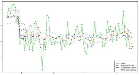
6.2 Estimated ωθ (left) and ωy (right) using MCMC approach. Small value of ωθ,1899 signal the break and small values ofωyin 1888 and 1964 signals outlying observation at the time . . . 65 6.3 Plot of filtered and smoothed values from Nile River data using SMC algorithm 65
6.4 Posterior estimates ofωθ(left) andωy (right) from Nile River data using SMC
algorithm . . . 66
6.5 Simulated time series with a potential outlier and structural break . . . 67
6.6 Plot of simulated data, filtered and smoothed values of the sates, θ, obtained via SMC approach . . . 68
6.7 Posterior estimates ofω’s from a simulated time series with a potential outlier and structural break obtained using SMC approach . . . 69
6.8 Monitoring the Effective Sample Size . . . 69
6.9 Plot of simulated data, filtered and smoothed values of the sates, θ, obtained using sequential MCMC . . . 70
6.10 Posterior estimates ofω’s from a simulated time series with a potential outlier and structural break obtained using sequential MCMC . . . 71
6.11 Detection of breaks and outliers from simulated data using (a)Shewhart,(b) CUSUM and (c) EWMA Chart . . . 72
6.12 Simulated data with linear trend and possible structural break . . . 73
6.13 Plot of simulated data, filtered and smoothed values . . . 74
6.14 Posterior estimates of (a)ωy,t, (b) ωθ,t,1 and (c)ωθ,t,2 . . . 74
6.15 Filtered and smoothed values of a time series with two potential outliers, one at the current timet = 181 . . . 76
6.16 Posterior estimates ofωy,t(left) andωθ,t(right) from a time series with distinct outliers at time t= 80 and the current timet = 181 . . . 76
6.17 Posterior estimates ofωy,t(left) andωθ,t(right) from a time series with distinct outliers at time t= 80 and the current timet = 181 . . . 77
6.18 Filtered and smoothed values of a time series with current at time t = 182 within the expected level . . . 78
6.19 Posterior estimates ofωy,t(left) andωθ,t(right) from a time series with distinct outliers at time t= 80 and at time t= 181. . . 79
6.20 An elaborate plot of posterior estimates of ωy,t showing presence of outliers
at timet = 80 and time t= 181 . . . 79 6.21 Posterior estimates ofωy,t(left) andωθ,t(right) from a time series with distinct
outliers at time t= 80 and at time t= 181. . . 80 6.22 Filtered and smoothed values of a time series with the two most current values
(t = 181,182) far from their expected values . . . 81 6.23 Posterior estimates ofωy,t(left) andωθ,t(right) from a time series with distinct
outlier at time t = 80 and two most current values ( t = 181,182) far from their expected values . . . 82 6.24 An elaborate plot of posterior estimates of ωθ,t showing potential structural
break at timet = 181 . . . 82 6.25 Posterior estimates ofωy,t(left) andωθ,t(right) from a time series with distinct
outlier at time t = 80 and two most current values ( t = 181,182) far from their expected values . . . 83 6.26 Top: A plot of filtered, smoothed and data from a time series with potential
outlier at t= 80, and two most current data far from their expected values Bottom left: Posterior estimates of ωy,t showing a distinct outlier at time
t= 80 Bottm right: Posterior estimates of ωθ,t indicate a potential structural
List of Abbreviations and Symbols
Symbols
y1:t indicates the observed data process (y1, y2,· · ·yt)
θ0:t indicates the Hidden Markov state process (θ0, θ1,· · · , θt)
ωt indicates the auxiliary state variable
νt indicates the degrees of freedom auxilliary variable defined on a set of
finite integers by associated probability vector π
X0:t indicates the state vector at time t, consisting of θ0:t, ν0:t and ω0:t
ψ parameter vector whose components include the state and
observation precision parameter λ, its associated mean and variances
a and b respectively, and probability vector π
N(µ, σ2) indicates a Gaussian distribution with mean µand variance σ2 N(x|µ, σ2) indicates the density function of Gaussian distribution with mean µ
and variance σ2 evaluated at x.
Gam(α, β) indicates a Gamma distribution with shape parameter α and rate parameter β
p(γ| · · ·) indicate the probability density function for γ given all other
unknowns and the data
p(X0:t, ψ|y1:t) indicate the joint posterior distribution for state vector X0:t and the
parameter vector ψ Abbreviations
ARMA Autoregressive Moving Average
ESS Effective sample size; see Chapter 4
EWMA Exponentially Weighted Moving Average; see Chapter 2
FFBS Forward Filtering Backward Sampling
GARCH Generalized Autoregressive Conditional Heteroscedasticity
MCMC Markov Chain Monte Carlo
SISR Sequential importance sampling with resampling
SMC Sequential Monte Carlo
Chapter 1
Introduction
Time series analysis involves data - often continuous measurements - collected or observed sequentially in time. We denote the univariate data byyt∈R where t∈ T is the time
indexing when the data was observed. The timet ∈ T can be discrete in which case T =Z or continuous time where nowT =R. For a multivariate data we have yt∈Rm whereyt =
(yt,1, yt,2,· · ·yt,m ) . For simplicity of the analysis we will consider only discrete time series.
Examples of time series data include stock market returns, oil production see Figure 1.1, data obtained from http://www.bp.com/en/global/corporate/about-bp/
statistical-review-of-world-energy-2013.html
The main aim of time series analysis is to create a mathematical model which will capture the underlying features of the observed data and help increase the understanding of
generating probabilistic mechanisms and the dynamic of the observed series. Once the model fits the data, the analyst most times may be interested also in parameter estimation and forecasting. During the analysis, stochastic homogeneity of the data is assumed. Disruptions of stochastic homogeneity of the data might be a signal of serious changes in the process observed. Such changes therefore, need to be detected as soon as data is
obtained. Time series data are often faced with such abrupt disruptions, some of which are temporary while others are permanent.
Structural time series model constitute of underlying states which include level, slope, seasonal, cyclic and irregular random components. The trend component represent long
Year 1970 1980 1990 2000 2010 0 200 400 600 800 1000 1200 Oil Production
(in millions tonnes)
● ● ● ● ● ● Africa Asia Pacific Europe & Eurasia Middle East North America S. & Cent. America
Figure 1.1: Global oil production from 1965 to 2012
term trend and usually constitute slope and intercept components. The seasonal component is the seasonal variation, cyclic component is repeated but non-periodic
fluctuations and the residual make up the irregular random components. Time series of UK gas consumptions from 1960 to 1980 is displayed in Figure 1.2.
Year 1960 1965 1970 1975 1980 1985 0 200 400 600 800 1000 1200 Gas consumption
(in millions of ther
ms)
Figure 1.2: UK Quarterly gas consumption, from 1960 to 1980 in Millions of therms
To demonstrate time series decomposition,the UK gas series is used broken down into various components. Results are shown in Figure 1.3. The first chart is the observed data process, a quarterly time series of length 108. The second chart is the trend of the data and the third is the seasonal components. The last chart is the remaining components after the trend and seasonal factors have been removed, usually referred to as irregular components.
200 600 1000 obser v ed 100 300 500 700 trend −150 −50 50 150 seasonal −200 0 100 0 5 10 15 20 25 random Time
Decomposition of additive time series
Figure 1.3: Time Series Decomposition
A basic structural time series model is of the form
yt=Tt+Ct+St+εt, ε ∼ N(0, σ2)
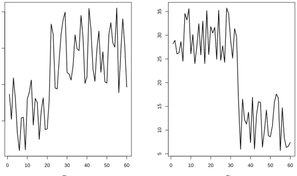
where T is the Trend, C is cyclic, and S is the seasonal component. Any structural times series model can easily be represented in state space form (West & Harrison, 1989) and the model could be formulated as a regression with time varying coefficients (Petris, Petrone, & Campagnoli, 2009). Details of the state space representation are presented in Chapter 3. Structural breaks (Harvey & Koopman, 2005) are permanent shifts which occur whenever there is a change or disruptions in one or more of these components(Perron, 2006). Figure 1.4 shows permanent upward and downward shifts in a time series.
0 10 20 30 40 50 60 30 35 40 45 Time 0 10 20 30 40 50 60 5 10 15 20 25 30 35 Time
Figure 1.4: Permanent upward shift (left) and downward shift (right) in a Time Series
These permanent disruptions might be a signal of serious changes in the observed process and they are of considerable importance in the analysis of time series variables. The structural breaks occurs for any number of reasons including economic crises, changes in institutional arrangements, war, policy changes and regime shifts. For example, the
combined effects of the Iranian revolution and the Iraq-Iran War in 1979 and 1980 caused a major drop in oil production in the Middle East, see Figure 1.1.
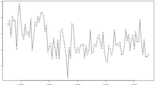
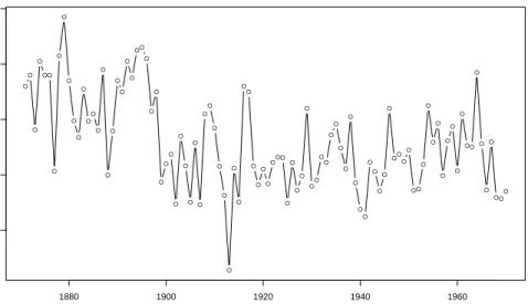
Figure 1.5 is plot of series of annual volume of discharge of the Nile River at Aswan from 1871 - 1970, given by (Cobb, 1978), which reveal a permanent drop of annual volume of discharge of the Nile River at Aswan from the year 1899. This sudden drop was largely due to the effect of Aswan dam, that was completed at that time
From the plot of UK quarterly gas consumption in Figure 1.2 there is a noticeable
● ● ● ● ●● ● ● ● ● ● ● ● ● ● ● ● ● ● ● ● ● ● ●● ● ● ● ● ● ● ● ● ● ● ● ● ● ● ● ● ● ● ● ● ● ● ● ● ● ● ●●● ● ● ● ● ● ● ● ● ● ● ● ● ● ● ● ● ● ● ● ● ● ● ●●● ● ●● ● ● ● ● ● ● ● ● ● ●● ● ● ● ● ●● ● Nile River Year 1880 1900 1920 1940 1960 600 800 1000 1200 1400
Figure 1.5: Annual volume of the Nile River from 1871 to 1970
increasingly important as both a theoretical research problem and a necessary component of applied data analysis.
An outlier or anomalous data point is defined as an observation in a dataset which appears to be inconsistent with the remainder of that set of data (Barnett & Lewis, 1994). Extreme values in a series may or may not be outliers and may arise as a result of either gross errors –due to faulty measurements, recording or typing errors –or they are true outliers.
Outliers occur frequently in measurement data and may have severe effects on model fitting and parameter estimation, leading to a mistaken conclusion and inaccurate predictions. It is therefore very important to identify them before modeling and analysis. Having said that, it is also worthy noting that, outliers often contain valuable information about the process under study or the data generating mechanisms. The outliers therefore require careful investigation and before considering possibly removing them, the researcher ought to understand why they occurred and the likelihood of their recurrence.
especially in safety critical environments (Ardelean, 2012). An outlier may indicate anomaly through which a significant flawed outcome may arise. In analysis of vital
variables of patients in intensive care for example, a small fault may lead to life threatening consequences. In manufacturing industries it is important to detect flaw in production line. While monitoring the usage of credit card, a sudden change in usage pattern may indicate credit card fraud. Similarly, a sudden change in monitoring process of mobile phone usage may indicate stolen mobile phone airtime. Other fields where outlier and structural breaks detection methods have been suggested include finance (Andreou & Ghysels, 2009) clinical trials (Penny & Jolliffe, 2001) and medical informatics (Laurikkala et al., 2000), voting irregularity analysis, severe weather prediction (Zhao, Lu, & Kou, 2003), geographic information systems (Shekhar, Lu, & Zhang, 2003), economics (Koop & Potter, 2000),(Perron, 2006).
In order to obtain a lucid statistical data analysis it is important, as an initial step, to detect outlying observations and structural breaks, if any, in the data.
Most existing outlier and structural detection techniques, however, deal with static data or are done off-line. There are different strategies to detect outlying observations including clustering algorithms, regression based statistics, likelihood ratio test and cumulative sum of observed residuals.
There is voluminous amount of work on structural breaks and outlier detection over the last 50 years in the statistics and other related fields literature, although the on-line approach - where the goal is to detect an outlier or whether a structural change has occurred, in real time- is minimal.
In today’s world where, in most cases, data arrive rather frequently and sequentially in time a fast, reliable and accurate detection methods are required for this online analysis. Methods that can be able to handle any level of noise and provide robustness against outliers. To that end, this dissertation’s focus is on sequential data and online detection of outliers and structural break, and my main objectives was primarily to
Design an algorithm to make inference sequentially for the model for outliers and structural breaks. The model used is decribed in details in Chapter 5
Implement the algorithm in a statistical software and
To obtain good results in practice on simulated and real data.
The dissertation is organized as follows: Chapter 2, we discuss various method that are available for detecting outliers and structural breaks in array of data and online. Chapter 3 emphasizes the State space models. We review the existing literature including the highly celebrated Kalman filter and Forward Filtering Backward Sampling (FFBS) algorithms . In Chapter 4 we discuss Sequential Monte Carlo methods, Chapter 5 we introduce the model for structural breaks and outlier for online data, Chapter 6 we evaluate our algorithm with simulated data and real data and provide some results. These results are compared with output from MCMC algorithm and finally the dissertation ends with some discussion in Chapter 7.
Chapter 2
Outliers and Structural breaks: Review
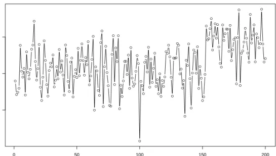
● ●● ● ● ● ● ● ● ● ● ● ● ● ● ● ● ● ● ● ● ● ● ● ● ● ● ● ● ● ● ● ● ● ● ● ● ● ● ● ● ● ● ● ● ● ● ● ● ● ● ● ● ● ● ● ● ● ● ● ● ● ● ● ● ● ● ● ● ● ● ● ● ● ● ●● ● ● ● ● ● ● ● ● ● ● ●● ● ● ● ● ● ●● ● ● ● ● ● ● ● ● ● ● ● ● ● ● ● ● ● ● ● ● ● ● ● ● ● ● ● ● ● ● ●●● ●● ● ● ● ● ● ● ● ● ● ● ● ● ● ● ● ● ● ● ● ● ● ● ●● ● ● ● ● ● ● ● ● ● ● ● ● ● ●● ● ● ● ● ●● ● ● ● ● ●● ● ● ● ● ● ● ● ● ● ● ● ● ● ● ● ● ● ● 0 50 100 150 200 18 20 22 Time
Figure 2.1: Time series data showing an outlier at time t= 100 and possible structural break at timet = 153
Most studies on outliers classify them as either (i) additive outlier - where only one observation is affected and after which the series return to its normal path, or
(ii)innovative outlier which influences subsequent observations from its initial position. There are various strategies and approaches which has been developed to deal with outliers and structural breaks in statistical data. Most of these methods are static batch-type
Sequential detection methods have also been proposed in some analysis, albeit minimally. Detection of outliers is simple when there is no serial dependence on the observations. In this case the procedures that involves detecting instabilities in mean and variances are of vital importance. The extreme observations -the very large or very small- are often treated to be inconsistent with the assumed generating mechanism or distribution and hence require to be tested for outlyingness. A number of outlier detection techniques over static data have been proposed (Barnett & Lewis, 1984), (Hodge & Austin, 2004).
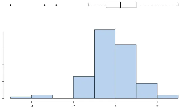
● ● ● Data Values Frequency −4 −2 0 2 0 10 20 30 40
Figure 2.2: Univariate data: The box plot identifies the outlying observations
The simplest and traditional statistical outlier detection technique is the use of the box plots. They provide graphical representation that allows the researcher to identify outlying observations in both univariate and multivariate data sets. The box plots make no
assumption of the distribution of the data and they plot, among others, the lower and upper extreme values. The outliers are identified as observations beyond these two extreme values. A univariate data set is displayed in Fig 2.2 by a skewed histogram and an overlaid box plot from which the three outlying observations are clearly identifiable. Figure 2.3
shows a basic scatterplot from bivariate data obtained from selected cities in US. A
negative correlation between mortality and education level is well captured and one of the superimposed box plots clearly uncovers the presence of an outlier.
● ● ● ● ● ● ● ● ● ● ● ● ● ● ● ● ● ● ● ● ● ● ● ● ● ● ● ● ● ● ● ● ● ● ● ● ● ● ● ● ● ● ● ● ● ● ● ● ● ● ● ● ● ● ● ● ● ● ● ● 9.0 9.5 10.0 10.5 11.0 11.5 12.0 800 900 1000 1100 1200 Education Mor tality ●
Figure 2.3: Outlier in a bivariate data
The distance-based approaches (Knorr, Ng, & Tucakov, 2000) computes and utilizes distance between two data points or examines the spatial proximity of each data point in the data space and if its proximity deviates considerably from the proximity of the other data then a data point is considered an outlier. These techniques do not make prior assumptions of the data distribution model. They are simple to implement but, since they are based on calculation of distances between all observations, they suffer from Curse of Dimensionality; that is, computational complexity increases as the dimension of data m
and number of observations T increases. The clustering algorithms such ask-Nearest Neighbors heirechical and k-means algorithms features prominently in this approach. Figure 2.4 shows some outliers from a popular dataset Iris using k-means clustering
● ● ● ● ● ● ● ● ● ● ● ● ● ● ● ● ● ● ● ● ● ● ● ● ● ● ● ● ● ● ● ● ● ● ● ● ● ● ● ● ● ● ● ● ● ● ● ● ● ● ● ● ● ● ● ● ● ● ● ● ● ● ● ● ● ● ● ● ● ● ● ● ● ● ● ● ● ● ● ● ● ● ● ● ● ● ● ● ● ● ● ● ● ● ● ● ● ● ● ● ● ● ● ● ● ● ● ● ● ● ● ● ● ● ● ● ● ● ● ● ● ● ● ● ● ● ● ● ● ● ● ● ● ● ● ● ● ● ● ● ● ● ● ● ● ● ● ● ● ● 4.5 5.0 5.5 6.0 6.5 7.0 7.5 8.0 2.0 2.5 3.0 3.5 4.0 Sepal.Length Sepal.Width + + + + + + Cluster center Outliers
Figure 2.4: Outliers with k-Means Clustering
Statistical-based approach (Rousseeuw & Leroy, 2005), assume data follows a certain statistical model. In this case, the probabilistic tests, based on the model, are carried out and outliers are identified as say, points that have a low probability to be generated by the overall distribution.
In many applications it is common for time series data to be serially dependent. There is high interest in current time series research to incorporate structural dependence of the observations in the analysis. This is the fundamental concept of this dissertation.
A significant literature exist which tests for structural breaks or non-linearity in time series. As hypothesis testing problem for detecting structural breaks, the null is set up to describe series with structural stability while the alternative contains one or more structural breaks.
2.1 Statistical Process Control (SPC)
The study of structural breaks in time series stemmed from quality control, but is now an integral part of a wide variety of fields. These applications include economics (Rodrigues & Rubia, 2011) and finance (Severin & Schmid, 1998), education, medicine (Bottle & Aylin, 2008), health services (Woodall, 2006).
SPC methods are used to detect when a stable process- one with fixed mean level and fixed variation- departs from stability. Most traditional diagnostics tools, like Shewhart control charts, popular in Statistical Process Control are used to define a standard of quality for manufacturing process and to determine whether the determined quality is being
maintained by the process. The most important factor is the variability in the quality of the finished product. No matter how much attention is paid towards quality of a product, a certain amount of variability is unavoidable and is a function of random forces and likely to be beyond control. Other methods include Change point detection (CPD) models whose goal is recognizing regime change events and adapting the predictive model appropriately. The Bayesian change point analysis assume a change point model of the parameters, integrating out the uncertainty in the parameters, rather than using a point estimate.
2.1.1 Quality Control Charts
The quality control charts, suggested by (Page, 1954) and detailed in (Hawkins & Olwell, 1998) and (Montgomery, 2007) were originally designed for industrial and manufacturing processes to define a standard of quality and determine whether that standard is being maintained by the process over time. The idea of standard control charts is to take the individual quality measures or statistics- usually means- of subsamples of these measures and plot them on a marked chart with control limits from the target value. It is on these plots that the unusual patterns or departures from state of statistical control will be
2.1.2 Shewhart charts
One of the most widely used is the Shewhart control charts (Shewhart, 1926) which monitor the production process and detect any significant deviation from a chosen quality characteristic of the products. A sample of fixed size is drawn at each regular time interval and desired statistic is computed. A sequence of such statistics are represented graphically in the form of a control chart. When a statistic falls outside of pre-determined control limits e.g. ’three-sigma control limits’, the production process, at that time, is said to be out-of-control and a warning sign is raised. See figure 2.5.
Shewhart charts are sensitive to large process shifts however the probability of these charts detecting small shift fast is quite small.
● ● ● ● ● ● ● ● ● ● ● ● ● ● ● ● ● ● ● ● ● ● ● ● ● ● ● ● ● ● ● ● ● ● ● ● ● ● ● ● ● ● ● ● ● ● ● ● ● ● ● ● ● ● ● ●● ● ● ● ● ● ● ● ● ● ● ●● ● ● ● ● ● ●● ● ● ● ● ● ● ● ● ● ● ● ● ● ● ● ● ● ● ● ● ● ● ● ● ●● ● ● ● ● ●●● ●● ● ● ● ● ● ● ● ● ● ● ● ● ● ● ● ● ● ● ● ● ● ● ●● ● ● ● ● ● ● ● ● ● ● ● ● ● ●● ● ● ● ● ●● ● ● ● ● ●● ● ● ● ● ● ● ● ● ● ● ● ● ● ● ● ● ●● 0 50 100 150 16 18 20 22 24 Time ● ● ● ● ● ● ● ● ● ● ● ● ● ● ● ● ● ● ● ● ● ● ● ● ● ● ● ● ● ● ● ● ● ● ● ● ● ● ● ● ● ● ● ● ● ● ● ● ● ● ● ● ● ● ● ●● ● ● ● ● ● ● ● ● ● ● ●● ● ● ● ● ● ●● ● ● ● ● ● ● ● ● ● ● ● ● ● ● ● ● ● ● ● ● ● ● ● ● ●● ● ● ● ● ●●● ●● ● ● ● ● ● ● ● ● ● ● ● ● ● ● ● ● ● ● ● ● ● ● ●● ● ● ● ● ● ● ● ● ● ● ● ● ● ●● ● ● ● ● ●● ● ● ● ● ●● ● ● ● ● ● ● ● ● ● ● ● ● ● ● ● ● ●●
Figure 2.5: Mean QC Chart
2.1.3 Cumulative Sum (CUSUM) charts
Another most widely used control charts is the cumulative sum (CUSUM) (Page, 1954) charts. They are procedures for mean and uses cumulative history, or the past information
of the process, to help in detecting small systematic departures from its normal and stable condition. These changes are detected easily and faster than in the standard Shewhart charts, however for large, abrupt shifts Shewhart chart detect much faster. The CUSUM are non-parametric and do not make use of a particular time series model fit.
The CUSUM charts are build on principles of Maximum Likelihood Estimation (MLE). The standard CUSUM chart for controlling the process mean takes samples from the process at a fixed interval and uses a control statistic based on cumulative sum of
differences between the sample mean and the target value. The procedure for CUSUM is as follows: Suppose the quality measurementsX1, X2, . . . are taken sequentially with time,
and assume that Xi is normally distributed with mean µ and variance σ2, that is
Xi ∼N(µi, σ2) i= 1,2, . . . and the variance σ2 is known and remains constant. The idea
is that, if the process is in control then any mean µi is equal to the target mean µ0. This is
the condition that need be monitored.
The 2-sided CUSUM chart is based on the cumulative statistics, Si and Ti, i= 1,2, . . .,
where
Si =max(0, Si−1+Zi−k)
Ti =min(0, Ti−1+Zi+k),
where Zi = (Xi
−µ0)
σ and k >0. The cumulative sums is given by Ci =
Pi
j=1Zj, i= 1,2, . . .
As the number of measurements are taken the probability that the CUSUM value may drift into extreme values increases. This is corrected by the reference value k = δσ2 where δ
the amount of shift in the process mean that we wish to detect. The process is out of control if either Si orTi exceed the control limit determined by a value h >0. The choice
of h is dependent on how sensitive the method is meant to be. The smaller it is the quicker will any departure from target be detected but also the more likely a false alarm will occur. In most cases h is chosen to be five times the process standard deviation or computed by
h= σ δln
1−β α
where α is the probability of false alarm and β is probability of failing to detect a shift in the mean when it has actually occurred. The CUSUM is expected to signal whenever SN ≥h orTN ≤ −h. The value N is popularly known as the run length
and defined as the number of measurements between each false alarm when the process is still in control. Its average value is known as the average run length (ARL).
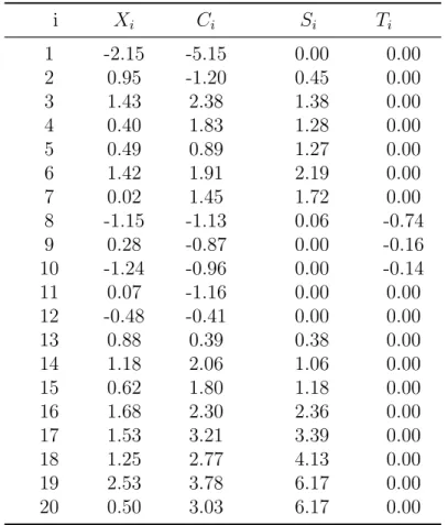
Example 1 To illustrate this consider series of 20 observations whose first 15 are sampled
from standard normal distribution and the rest are drawn from a normal distribution with mean µ= 1 andσ = 1. We want to detect the upward shift in mean, so δ= 1 and therefore
k = 0.5. From previous discussion h= 5
The simulated values are shown in the Table 2.1
The CUSUM chart for this data is shown in Figure 2.6 and it is clear that the out-of-control signal is given after the 18th observation.
● ● ● ● ● ● ● ● ● ● ● ● ● ● ● ● ● ● ● ● 5 10 15 20 −6 −4 −2 0 2 4 6 Cum ulativ e Sum ● ● ● ● ● ● ● ● ● ● ● ● ● ● ● ● ● ● ● ● Upper cusum Lower cusum Si Ti
Table 2.1: Simulated data and associated CUSUM statistics i Xi Ci Si Ti 1 -2.15 -5.15 0.00 0.00 2 0.95 -1.20 0.45 0.00 3 1.43 2.38 1.38 0.00 4 0.40 1.83 1.28 0.00 5 0.49 0.89 1.27 0.00 6 1.42 1.91 2.19 0.00 7 0.02 1.45 1.72 0.00 8 -1.15 -1.13 0.06 -0.74 9 0.28 -0.87 0.00 -0.16 10 -1.24 -0.96 0.00 -0.14 11 0.07 -1.16 0.00 0.00 12 -0.48 -0.41 0.00 0.00 13 0.88 0.39 0.38 0.00 14 1.18 2.06 1.06 0.00 15 0.62 1.80 1.18 0.00 16 1.68 2.30 2.36 0.00 17 1.53 3.21 3.39 0.00 18 1.25 2.77 4.13 0.00 19 2.53 3.78 6.17 0.00 20 0.50 3.03 6.17 0.00
2.1.4 Exponentially Weighted Moving Average (EWMA)
This control scheme, introduced by (Roberts, 1959), utilizes the statistic At,
At=φyt+ (1−φ)At−1, 0< φ≤1, t= 1,2, . . .
and some determined upper and lower limits. The sequentially observed data yt can be the
actual observed value or the sample mean from designed sampling strategy from the process. A0 is often taken to be the process target value, µ0 . The control limits are
determined as follows: µ0±Lσ s φ (2−φ)(1−(1−φ) 2t)
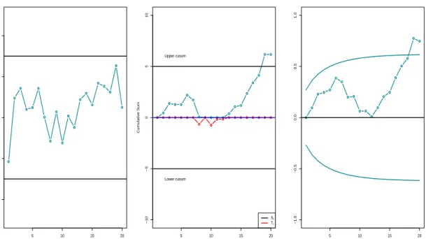
where Lis the width of the control limits. Both φ and L are chosen after specifying desired ARL and the shifted anticipated. The EWMA have proved to be effective against small shifts but, just like CUSUM, does not react quickly to large shifts as compared to Shewhart chart. The comparison of the 3 charts is displayed in Figure 2.7.
Example 2 We use the same data as in Example 1, and let µ0 = 1, φ = 0.1, L= 2.7. The
results are displayed in Figure 2.7
In a serially dependent processes, parametric models are often used to describe explicitly the structural dependence assumed in the data while at the same time seek potential structural breaks. Most commonly used model are class of Autoregressive Moving Average (ARMA) Tsay (1988) and Generalized Autoregressive conditional Heteroscedasticity (GARCH)(Bollerslev, 1986) type models.
● ● ● ● ● ● ● ● ● ● ● ● ● ● ● ● ● ● ● ● 5 10 15 20 −4 −2 0 2 4 (a) ● ● ● ● ● ● ● ● ● ● ● ● ● ● ● ● ● ● ● ● 5 10 15 20 −10 −5 0 5 10 (b) Cum ulativ e Sum ● ● ● ● ● ● ● ● ● ● ● ● ● ● ● ● ● ● ● ● Upper cusum Lower cusum Si Ti ● ● ● ● ● ● ● ● ● ● ● ● ● ● ● ● ● ● ● ● 5 10 15 20 −1.0 −0.5 0.0 0.5 1.0 (c)
Figure 2.7: (a)Shewhart,(b) CUSUM and (c) EWMA Chart
2.2 ARMA and GARCH models
The ARMA model for outliers proposed by Box and Tiao (1975) involves the unobservable
Zt related to observed series yt by the function
yt=f(t) +Zt
where f(t) is parametric function that represent exogenous disturbance of Zt, and the Zt is
modelled by ARMA model
φ(B)Zt=ϕ(B)at
where φ(B) = 1−φ1B−φ2B2, . . . φpBp and ϕ(B) = 1−ϕ1B−ϕ2B2. . . ϕqBq are
Autoregressive and Moving Averages polynomials inB of degrees pand q respectively. B is backwardshift operator such that BZt=Zt−1, {at} is a sequence of independent normally
The function f(t) is designed f(t) = ω0 ω(B) δ(B)ξ (d) t
where ω(B) = 1−ω1B−ω2B2−. . .−ωsBs and δ(B) = 1−δ1B −δ1B−. . .−δrBr are
polynomials in B with degrees s and r respectively. ω0 is the magnitude of the outlier or
the initial jump of the series and ξt(d), is an indicator variable that signifies the occurrence of outlier or structural break at point d .
For an outlier (additive) model,ω(B) = δ(B)
ξt(d) = 1, t=d 0, t6=d
To detect a structural change, theδ(B) is taken to be equal to 1 and
ξ(td) = 1, t≥d 0, t < d
Other special cases for ω(B)/δ(B) are discussed in (Box & Tiao, 1975) and (Tsay, 1988) In most cases the parameters involved in these models are usually unknown and practically they are estimated from the data. Outliers and structural breaks problems have been considered as hypothesis tests with null describing the model with no outlier or breaks. The alternative contains one or multiple outliers or breaks. Under null hypothesis, the maximum likelihood estimates (MLE) are consistent, and often suggested, and can
therefore be used to estimate the parameters and to design relevant test statistics (Aue & Horv´ath, 2013). These test statistics are used to identify outliers or structural breaks if any. The Weighted Likelihood estimation method also provide efficient and robust estimators for ARMA models. The idea of outlier detection using likelihood ratio test
-when the location and the type is known- in autoregressive processes was first proposed by (Fox, 1972)
(Ardelean, 2012) proposed the use of the (GARCH) process in detecting outliers and structural breaks in time series. A real-valued discrete time stochastic process (Xt)t∈Z is a
GARCH(p,q) process if:
Xt|Ft−1 =σtεt, σt2 = (σt(ψ))2 =α0+ p X i=1 αiXt2−i+ q X i=1 βiσ2t−i
where Ft denote the information set of the process up to timet, and the innovations εt is
sequence of i.i.d random variables from some distribution G with EG(εt) = 0 and
EG(ε2t = 1). ψ = (α0, α1, . . . α0, β1, . . . βq), α0 >0, αi ≥0, i= 1, . . . p and βj ≥0, j = 1, . . . q
Following (Ardelean, 2012), both the outliers can be modeled as follows: additive: Yt =Xt+εIt(τ) Xt|Ft−1 ∼N(0, σt2−1) σt2 =α0+ p X i=1 αiXt2−i+ q X i=1 βiσt2−i innovational Yt=Xt+εIt(τ) Xt|Ft−1 ∼N(0, σt2−1) σt2 =α0+ p X i=1 αiYt2−i + q X i=1 βiσt2−i
observed process, ε ∈R is the size of the outlier occurring at time time τ ∈Z, and It(τ) is
an indicator function which is equal to 1 if τ =t and 0 otherwise. It is obvious from the relation that GARCH(1,1) parameterizes the conditional variance in terms of ARMA(1,1) To test for occurrence of outlier and structural breaks simultaneously the model is modified such that Yt=Xt+ε1It(τ) σt2 =α0+ p X i=1 αiXt2−i+ q X i=1 βiσt2−i+ p X i=1 ε1+iIτ−i
where ε1 is the size of the outlier occurring at time τ and ε2, . . . εp+1 is the size of each
structural break. Due to the ARMA representation, the parameters in the model
ψ = (α0, α1, . . . αp, β1, . . . βq, ε1, . . . εp+1) can be estimated using MLE. By taking
ˆ
ψ0 = ( ˆα0,αˆ1, . . .αˆp,βˆ1, . . . ,βˆq) to be the restricted MLE and
ˆ
ψ1 = ( ˆα0,αˆ1, . . .αˆp,βˆ1, . . . ,βˆq,εˆ1,εˆ2, . . . ,εˆp+1) to be the unrestricted MLE, the likelihood
ratio test statistic, for testing the hypothesis of no outlier or break at time τ, that is
Ho :ε1 =ε2 =. . .=εp+1 = 0
can be computed, for every τ ≤T, as
λτ = 2(logL( ˆψ0)−logL( ˆψ1))∼χ2(p+1)
2.3 Regression models
Regression models have also been used in modeling outliers and structural breaks. Consider the general linear regression model
Yt =Xtβ+t, t
iid
where Xt= (1, X1,t, . . . , Xp,t) is a vector of the intercept and p non-random explanatory
variables and β= (β0, β1, . . . , βp)T are the regression coefficients.
These unknown coefficients are usually estimated by ordinary least-squares method
ˆ β = (XTX)−1XTY, Y = Y1 .. . YT , X= X1 .. . XT
Outliers with respect to the explanatory variables are called the leverage points; they can have adverse effect on the regression model. Leverage points do not necessarily correspond to outliers and also their response variable need not be outliers.
The predicted or the fitted values, ˆY are computed using the data matrix and the estimated coefficients
ˆ
Y =X ˆβ
The ordinary residuals ˆ, is the difference between the predicted and the observed values
ˆ
=Y −Yˆ
are the widely used measures in identifying outliers in regression models. The techniques available involve deleting rows with suspicious observation or leverage point and compute statistics thereafter. Examination is then done on the effect of each row deletion on the estimated coefficients and their estimated covariance structure, the predicted values, and the residuals. Most common outlier diagnostics involve statistics mostly computed using the estimated regression coefficients, are briefly discussed below
2.3.1 Hat Matrix
The hat matrix denoted by H and defined as
H =X(XTX)−1XT
plays an important role in identifying outliers or leverage points. The diagonal elementshii
of H being the amount of leverage exerted by the ith observation on theith fitted value.
The ith observation is an influential point when hii exceeds 2p/T, where pis the rank of the X matrix.
2.3.2 Cook’s Distance
Cook’s Distance statistic proposed by (Cook, 1979)
Di =
( ˆY(i)−Yˆ)T( ˆY(i)−Yˆ) ps2
follows Fp,T−p distribution, where ˆY(i)=X ˆβ(i) with βˆ(i) as the vector of estimated
regression coefficients with the ith row deleted, s2 is the estimator of σ2. The D
i statistic
has a cut-off of 4/p and large values indicates an outlier or leverage point.
2.3.3 DFFITS
The DF F IT Si is the difference between the fitted response variable, ˆYi from the full model
and the predicted values ˆYi(i) obtained after removing the ith observation from the dataset.
DF IT T Si = ˆ Yi−Yˆi(i) q ˆ σ2 (i)hii
where hii is the ith diagonal element of the hat matrix, H. A value is considered suspicious
|DF IT T S|>2pp/T
2.3.4 DFBETAS
This is the change in the estimate of regression coefficients that would occur if the ith row
is removed. DF BET ASj(i)= ˆ βj −βˆj(i) q ˆ σ2 (i)(XTX) −1 jj
The cut-off value for DF BET AS for small to medium data set is 1 while in large data sets a value |DF BET AS|>2/√T is considered suspicious.
These numerical measures though effective in case of existence of single outlier, may fail if more than one outliers exists. Moreover, when data is collected over time, serial
dependence is a significant component and therefore model assumption of independent errors is violated and model can’t be used.
However if we allow for time-varying coefficients the now generalized regression, discussed in Chapter 3, can be used to detect outliers and structural breaks in time series data.
2.4 Some Multivariate Outlier Detection Methods
2.4.1 Static data
In a multivariate data the classical approach in detecting outliers is to consider the
distance of a each observation as well as the shape and the size of the data. The shape and size of multivariate data are expressed by the covariance matrix.
The basic statistical measure for outliers detection and which takes also into account the covariance matrix is the Mahalanobis distance (Mahalanobis, 1936). The statistic is computed using the estimate of multivariate location- usually the mean- and the sample
sample from multivariate normally distributed data with mean vector µand covariance matrix Σ, the Mahalanobis’ distance
M Dt = (yt−µˆ)TΣˆ−1(yt−µˆ)
12
identifies the observation that are very far from the centre of the data cloud or the centroid. A test statistic for M Dt is given by
(T −m)T
(T2−1)mM Dt
which is approximate F distribution with degrees of freedom m and T −m.
Since the sample estimates ˆµand ˆΣ are very sensitive to outliers, which the M Dt is meant
to identify, they need to be estimated using a robust procedure in order to provide a credible and reliable criterion. There is significant literature on robust estimation of M Dt
(Franklin, Thomas, & Brodeur, 2000), (Pe˜na & Prieto, 2001)
Due to calculations of the covariance matrix estimate, ˆΣ, the Mahalanobis distance is computationally expensive, with runtimeO(T2m), for large and high dimensional data sets. Another popular statistical measure is the Euclidean distance
dx,y = v u u t T X i=1 (xi−yi)2
Both Mahalanobis and Euclidean distance measures are important ingredients in proximity based techniques for outlier detection, such as clustering and k-Nearest Neighbors
algorithms.
2.4.2 Time series data
following the vector ARMA (VARMA)model
Φ(B)Zt=ϕ(B)at
where Φ(B) = 1−Φ1B −Φ2B2−. . .−ΦpBp and ϕ(B) = 1−ϕ1B −ϕ2B2−. . .−ϕqBq
are m×m matrix polynomial of degrees p and q. B, like in the univariate case, is a
backward shift operator such that BZt=Zt−1 and at= (a1,t, a2,t, . . . am,t)T is a sequence of
uncorrelated Gaussian random vectors with mean 0 and positive-definite covariance matrix
Σ Zt are related to the observed series Yt= (Y1,t, Y2,t, . . . , Ym,t)T by the function
Yt=Zt+α(B)ωξt(d)
whereω = (ω1, ω2, . . . , ωm)T is the size of the outlier, ξ
(d)
t is the indicator variable such that
ξt(d) = 1 ift=d and zero otherwise. The matrix α(B) define the type of outlier with
α(B) =I indicating an additive outlier and if α(B) =ϕ(B)/Φ(B) indicates a multivariate structural break. Other special cases of α(B) are discussed in (Galeano et al., 2006). (Atkinson, Koopman, & Shephard, 1997) used the Gaussian State space model, details given in Chapter 3, with regression variables through which shocks- outliers or breaks- were introduced.
Chapter 3
State Space Model
3.1 General State Space Model
State space models provide an effective basis for practical time series analysis and forecasting (Durbin & Koopman, 2012), (Harrison & West, 1997), (Aoki, 1990).
The models are highly applicable in various fields and disciplines including computer vision (i.e. tracking), control theory, econometrics, population dynamics. The state space model involves two processes: the latent or unobserved Markov state process, {θt}t≥1, θt ∈Rp
and the noisy observation process {yt;t∈N}, yt ∈Rm that is related to the state process.
The state space model is specified through descriptions of the sampling distribution, the state vector evolution, and the initialization of the state vector. See equations 3.1 and 3.2 The state vector contains all relevant information required to describe the system under investigation. It may contain regression variables or components of time series such as level, trend, seasonal or cyclic components. In tracking problems, for example, this information could be related to the kinematic characteristics of the target object. In an econometric problem, it could be related to monetary flow, interest rates, inflation, stock markets etc.
Conditional probability
The conditional probability of a variable a given b is defined
p(a|b) = p(a, b)
from where Bayes’ rule follows quickly
p(a|b) = p(b|a)p(a)
p(b)
or more conceptually
P osterior= Likelihood×P rior
M arginal likelihood (evidence)
Conditional Independence
A variable a is conditionally independent of b given c, denoted bya⊥b |c, if
p(a|b, c) =p(a|c).
Lety1:t:= (y1, y2. . . , yt) represent all the data or information up to and including time t,
and θ0:t := (θ0, . . . ., θt) be state representation up to time t. The state space model are
based on two very important assumptions:
conditional on the parameter ψ state process {θt}t≥0 is a Markov process; that is p(θt|θ0:t−1, ψ) =p(θt|θt−1, ψ).
yt depends only onθt and conditional on the state process {θt}t≥0, the{yt}’s are
independent. p(yt|θ0:t, y1:t−1) =p(yt|θt)
This conditional dependence is demonstrated in Figure 3.1. The general state space model is defined by these two equations
yt|θt, ψ ∼p(y|θt, ψ) (3.1)
θt|θt−1, ψ ∼p(θt|θt−1, ψ) (3.2)
θ0 θ1 y1 θ2 y2 · · · θt−1 yt−1 θt yt θt+1 yt+1 · · ·
Figure 3.1: Structural dependence of state space model
The goal in statistical inference on state space models is, based on the available data, to estimate the unobserved states and the unknown parameters in the model and predict the states and/or future observations. The estimation of the state vector entails filtering and smoothing problem. This inference is achieved by computing conditional and or marginal distributions based on the joint distribution
p(θ0:t, ψ, y1:t) =p(ψ)p(θ0|ψ) t Y j=1 p(θj|θj−1, ψ) | {z } p(θ0:t|ψ) t Y j=1 p(yj|θj, ψ) | {z } p(y1:t|θ0:t,ψ) (3.3)
Given data up to time t and assuming thatψ is known, the marginal distribution
{p(θt|y1:t)}t≥1 also known as the filtering density is obtained via Bayes’ rule as
p(θt|y1:t) =
p(yt|θt)p(θt|y1:t−1) p(yt|y1:t−1)
To obtain an estimate of the states joint distribution p(θ0:t|y1:t), again, by Bayes’ rule we
have, p(θ0:t|y1:t) = p(θ0:t, y1:t) p(y1:t) = p(yt|θt)p(θt|θt−1)p(θ0:t−1|y1:t−1) p(yt|y1:t−1)
The marginal likelihood p(y1:t) can be obtained as
p(y1:t) =
Z · · ·
Z
p(θ0:t, y1:t)dθ0:t
available data. The smoothing is achieved by the density p(θt|y1:T) fort < T, p(θt|y1:T) = p(θt|y1:t) Z p(θt+1|θt) p(θt+1|y1:t) p(θt+1|y1:T)dθt+1
For predicting or forecasting future states and observations, the k−steps (k ≥ 1) predictive densities for the states and observation respectively, is given by
p(θt+k|y1:t) = Z p(θt+k|θt+k−1)p(θt+k−1|y1:t)dθt+k−1 p(yt+k|y1:t) = Z p(yt+k|θt+k)p(θt+k|y1:t)dθt+k
Parameter learning is achieved via the density p(ψ|y1:t).
For linear Gaussian models, all posteriors are Gaussian and the above quantities can be computed analytically by using well established algorithms which include Kalman filter and smoother (Kalman et al., 1960) and the Forward Filtering Backward Sampling (FFBS) (Fr¨uhwirth-Schnatter, 1994). For non-linear and non-Gaussian models, computing the above quantities in closed form is analytically intractable, and numerical approximation, in particular Markov Chain Monte Carlo (MCMC), is required. However for online inferences where data arrive rapidly and frequently and hence fast and efficient updates of posterior quantities is requiredMCMC are ineffective.
3.2 Dynamic Linear Model (DLM)
Also known as Gaussian State Space Model, DLM is a class of state space models where equations (3.1) and (3.2) both are linear and Gaussian (West & Harrison, 1989), (Harrison & West, 1991) (Harrison & West, 1997). The model is specified by initial distribution
θ0 ∼ N(m0, C0) and the equations
yt =Ftθt+vt vt∼ N(0, Vt) (3.4)
θt =Gtθt−1+wt wt ∼ N(0, Wt) (3.5)
where Ft and Gt are known m×pand p×p transition matrices. The possible
time-dependent quantities Ft, Gt, Vt and Wt may depend on a parameter vectorψ.
By allowing for time-varying coefficients we can show that DLM is a generalization of linear regression model,
yt =Xtβt+t, t iid
∼ N(0, σt2), t= 1,2, . . . , T
where Xt= (1, X1,t, . . . , Xp,t) is a vector of the intercept and p non-random explanatory
variables and βt= (β0,t, β1,t, . . . , βp,t)T and we model evolution of coefficients
βj,t =βj,t−1+wj,t, j = 0,1, . . . , p
which is a DLM with Ft = [Xt], θt= [β0,t, β1,t, . . . , βp,t]T, Vt =σt2, and G=Ip, identity
matrix. (Petris et al., 2009)
The random walk plus noise also known as the local level model
yt=γt+vt vt∼ N(0, V)
γt=γt−1+wt wt∼ N(0, W)
3.2.1 Structural Time Series
Structural time series model is a linear combination of a random error component, ε with zero mean and a constant variance σ2and at least one of the three structural components, namely; the trend (T), cycle (C), and seasonal (S) components.
The basic structural time series model is shown below
yt =Tt+Ct+St+εt, εt∼ N(0, σ2) t = 1, . . . , T
Any structural model can be represented as DLM. For example, the locally linear trend model which is of the form
yt=Tt+εt, εt∼ N(0, σ2) t= 1, . . . , T (3.6)
and the linear trend is quickly derived from the deterministic function
Tt=Tt−1+ρt−1+ϑt (3.7a)
ρt=ρt−1 +ξt (3.7b)
where the innovations ϑt with zero mean and variance σϑ2 account for vertical or the
upward and downward shift of the trend. The innovations ξt have zero means and variance
σξ2 and they account for the trend’s change in slope. These innovationsϑt and ξt as well as
εt are mutually uncorrelated.
Using the equations (3.6), (3.7a) and (3.7b) we have a DLM with
G= 1 1 0 1 , θt= Tt ρt , F = 1 0 , W = σ2 ϑ 0 0 σξ2 , V =σ 2 and ψ = (σ2, σϑ2, σξ2)
3.2.2 ARMA representation
A significant number of state space representations for ARMA models exist. For detailed discussion on these representations, see (Petris et al., 2009), (Brockwell & Davis, 2009), (Kitagawa & Gersch, 1996), (Kedem & Fokianos, 2002). To illustrate, lets consider the data yt=xt+vt, vt ∼N(0, Vt) wherext is unobserved autoregressive process of order p ;
xt=Ppi=1φixt−i+t, with t∼N(0, σ2t). This is a DLM with
Gt= φ1 φ2 φ3 · · · φp−1 φp 1 0 0 · · · 0 0 0 1 0 · · · 0 0 .. . ... ... . .. 0 ... 0 0 · · · 1 0 , θt= xt xt−1 xt−2 .. . xt−p+1 , wt= t 0 0 .. . 0 Ft = [1,0,0, . . . ,0,0] and ψ = (φ1, φ2, . . . , φp, Vt, σ2t)
Since many linear models including ARMA models admit state space representation, the statistical inference on state space models can be applied to both stationary and
non-stationary data. Moreover, the state space models provides components that are easier to interpret unlike those from ARMA models.
When DLM is fully specified the state estimation, smoothing and or predictions as well as observation predictions, can be carried out by using the Kalman Filter and Smoother and FFBS algorithms. However when ψ is unknown, numerical methods and in particular the Monte Carlo methodsare required.
3.2.3 Kalman Filter
Given the information available at time t, the Kalman filter(Kalman et al., 1960) is a set of recursion equations- the predictions and updating equations- for determining optimal estimates of the state vector θt.
First, let mt =E(θt|y1:t) be the optimal estimator of θt based on information up to time t,
and Ct=E[(θt−mt)(θt−mt)
0
|y1:t] be the mean square error (MSE) matrix of mt.
The prediction step takes place prior to arrival of the data at time t, and involves predicting the states
p(θt|y1:t−1) = Z
p(θt−1|y1:t−1)p(θt|θt−1)dθt−1
Given, at time t−1, that θt−1 ∼N(mt−1, Ct−1), then from (3.4) and (3.5), it follows
quickly that the parameters for the predictive distribution of θt, given the information up
to timet−1, will be p(θt|y1:t−1)∼ N(m∗t, C ∗ t) where m∗t =E(θt|y1:t−1) = Gtmt−1 Ct∗ =E[(θt−mt−1)(θt−mt−1)T|y1:t−1] =GtCt−1GTt +Wt
and the corresponding optimal predictor of yt given all the information up to time t−1 is
yt|t−1 =E(yt|y1:t−1) =Ftm∗t
=FtGtmt−1
Once the new observationyt become available, the prediction error
et=yt−yt|t−1 =yt−FtGtmt−1 and its MSE
E(eteTt) = Qt=FtCt∗F
T
t +Vt
and the states updating step is defined, by Bayes formula
p(θt|y1:t) =
p(yt|θt)p(θt|y1:t−1) p(yt|y1:t−1) ∝ N(θt|mt, Ct)
with optimal predictor ofθt and its MSE matrix computed as follow:
mt=m∗t +C ∗ tF T t Q −1 t et Ct=Ct∗−C ∗ tF T t Q −1 t FtCt∗
3.2.4 Forward Filtering Backward sampling (FFBS)
Given all the data up to time t =T, we may be interested in computingp(θ0:T|y1:T).
Forward Sampling
This is achieved through Kalman Filter and computes the normal distribution
p(θt|y1:t) at eacht = 1,2, . . . , T
At time t =T: we sample θT∗ from p(θT|y1:T)
Fort =T −1, T −2, . . . ,0 : sample θ∗t from normal distribution p(θt|y1:t, θ∗t+1)
The desired output from the FFBS is the sequence θ∗T, θ∗T−1, . . . , θ0∗
3.2.5 MCMC in DLM
Inference on DLM with unknown parameters can be carried out by using MCMC approach. Again we letψ, be the vector of unknown parameters in the DLM. The inference will be based on the posterior distribution p(θ0:T, ψ|y1:T) whose decomposition is as follows
p(θ0:T, ψ|y1:T) = p(θ0:T|y1:T, ψ)p(ψ|y1:T)
It is logical, therefore, to use Gibbs sampling technique to sample iteratively from this posterior distribution,
starting with priorψ =ψ∗
Apply FFBS algorithm to draw smoothed state vector Θ∗ = (θT∗, θT∗−1, . . . , θ∗0) from
p(θ0:T|ψ∗, y1:T)
Draw new value ofψ∗ from p(ψ|Θ∗, y1:T)
Chapter 4
Sequential Monte Carlo (SMC) Methods
In many time series the data do arrive rather frequently and sequentially in time and one is interested in estimating recursively, in real time, the evolving posterior distribution.
Markov Chain Monte Carlo (MCMC) methods, though useful for off-line or batch inferences, are ineffective or of limited use for online inferences.
SMC are Monte Carlo technique that have been developed to deal with sequential or online inferences (Doucet, De Freitas, Gordon, et al., 2001). SMC techniques have been developed in a wide range of disciplines (e.g. missile tracking, stock market, medical monitoring) and go under many names: Particle filtering, Bootstrap filtering, the condensation algorithm, Interacting particle approximations, Survival of the fittest among others.
SMC is a ’divide and conquer’ approach that evaluates the full posterior by dividing it up into one time step at a time. That is, we want to compute p(θ0:t, ψ|y1:t) sequentially in time
t. First we compute p(θ0:1, ψ|y1) at time t = 1, then p(θ0:2, ψ|y1:2) at time t = 2 and so on.
Each target distribution is approximated by weighted Monte Carlo samples known as particles. This relation is denoted as
θ0:(i)t, ψ(i), w(ti) Ni=1 ∼p(θ0:t, ψ|y1:t) where N 1,w(ti) >0, Pi=1 N w (i) t = 1.
as N → ∞. That is, for any p-integrable function Φt:Rt×p →R N X i=1 w(ti)Φt(θ0:(i)t) a.s −→ Ep(Φt) = Z Φt(θ0:t)p(θ0:t|y1:t)dθ0:t (4.1) as N → ∞.
This strategy makes SMC technique fast and thus ideal for online inferences where fast and efficient updates of posterior quantities and forecasts are necessary to deal with high
frequency incoming data.
The fundamental concepts in SMC are Bayesian inference, Monte Carlo samples, importance sampling, and resampling.
We now briefly describe two fundamental concepts in SMC; the importance sampling and the resampling technique. The mechanisms through which the particles evolve.
4.1 Importance sampling
It is generally impossible to sample fromp(.) therefore we approximate our target
distribution p(.) with a proposal density q(.), also called the importance density, which is easy to sample from. The goal is to approximate the expected value of an arbitrary function g(x) using the underlying probability density p(.) and the proposal density. Assume that at time t-1, we have particles{θi
0:t−1} which have been sampled from a
proposal densityqt−1(θ0:t−1). Since they are not samples from the target density, they are
weighted with weights given by
w(ti−)1 ∝ pt−1(θ (i) 0:t−1) qt−1(θ (i) 0:t−1)
Assume we are interested in finding the expected value of an arbitrary function g(θ), with respect to p(θ). By definition Ep(θ)[g(θ)] = Z g(θ)p(θ)dθ= Z g(θ)p(θ) q(θ)q(θ)dθ (4.2) =Eq(θ)[g(θ) ˆw(θ)] (4.3) ≈1 N N X i=1 g(θ(i)) ˆw(i) (4.4)
where θ(i), i= 1, . . . , N is drawn from q(θ) and ˆw(θ) = p(θ)
q(θ) is the importance weights
function. The importance weights function is usually known up to proportionality constant, ¯w(θ) = kwˆ(θ) wherek is independent of θ
k = Z kp(θ)dθ = Z ¯ w(θ)q(θ)dθ =Eq(x)[ ¯w(θ)]
Now we can re-write equation (4.3) as
Ep(θ)[g(θ)] =Eq(θ)[g(θ) ¯ w(θ) k ] = Eq(θ)[g(θ) ¯w(θ)] Eq(x)[ ¯w(θ)] ≈ PN i=1g(θ (i)) ¯w(i) PN i=1w¯(i) = N X i=1 g(θ(i))w(i) where w= ¯w(i)/PN j=1w¯ (j).
A good approximation of p(θ) is therefore
ˆ p(θ) = N X i=1 w(i)δθ(i) (4.5)
where δx is the Dirac delta mass at x.
At time t, the weighted Monte Carlo approximation to p(θ0:t, ψ|y1:t) is given by
ˆ p(θ0:t, ψ) = N X i=1 w(ti)δ(θ(i) 0:t,ψ(i)) where: w(ti) = ¯wt(i)/PN j=1w¯ (j) t and ¯wt= p(θ(0:i)t,ψ(i)|y 1:t) q(θ(0:i)t,ψ(i)|y 1:t)
If we use a structured proposal distribution, and assuming that ψ is known
qt(θ0:t|y1:t) =q0(θ0)q1(θ1|θ0, y1)q2(θ2|θ1, θ0, y1:2), . . . , qt(θt|θ0:t−1, y1:t)
=qt−1(θ0:t−1|y1:t−1)qt(θt|θ0:t−1, y1:t)
Since θ0:(i)t−1|y1:t−1 ∼qt−1(θ0:t−1|y1:t−1) is available, then we only need to sample
θ(ti)|θ0:(i)t−1, y1:t∼qt θt|θ
(i) 0:t−1, y1:t
to obtain θ0:(i)t|y1:t∼qt(θ0:t|y1:t)
and the un-normalized weights, ¯wt(i) are updated according to
¯ w(ti) = p(θ (i) 0:t|y1:t) q(θ0:(i)t|y1:t) = p(yt, θt|θ0:t−1, y1:t−1)p(θ0:t−1|y1:t−1) qt|t−1(θt|θ0:t−1, y1:t)qt−1(θ0:t−1|y1:t−1) =wt(−i)1p(yt|θt)p(θt|θt−1) qt|t−1(θt|θt−1, y1:t)
4.2 Resampling and auxiliary index
One major problem with particle filter is particle degeneracy. After a few iterations, most particles have negligible weight and the weight is concentrated on few particles only. The other problem is the loss of diversity or sample impoverishment where particles with high
weight are selected more and more often while the others die out slowly. To counter these problems resampling of the particles is recommended. The technique involves sampling new particles, with replacement from a weighted empirical measure related to the current particles. Resampling eliminates particles with low weights and chooses more particles in high probability regions of the state space.
Resampling too often will decreases the number of distinct particles and do increase the Monte Carlo variance of the estimator. However, resampling also reduces the variances of estimates at a later stage. It is important therefore to resample but do so only when it is absolutely necessary. Deciding when to resample is a crucial part of the algorithm and its usually determined by assessing the quality of the current particles. The resampling is done whenever this criterion is above or below a certain predetermined threshold. By doing this, a reasonable number of contributing particles is maintained.
The most commonly used criterion is the effective sample size(ESS). This approach was originally proposed in (Kong, Liu, & Wong, 1994) with idea that the need of resampling increases with increase of the variance of importance weights. Since this variance is unknown, the ESS is used in its place. ESS provides an approximation of the number of independent samples from the target distribution that would be required to provide an estimate of comparable variance.
The simplest way to perform resampling consists of sampling the N new particles from the weighted distribution ˆpN
t ; the resulting NtN are distributed according to a multinomial
distribution of parameters wtN.
Other sampling schemes include Stratified resampling (Kitagawa, 1996) and residual resampling (Douc & Capp´e, 2005). These reduce the variance ofNN
t relatively to that of
4.3 Convergence results
Numerous convergence results are available for SMC methods (Crisan & Doucet, 2002) (Del Moral, 2004). Again we take Φt:Rt×p →R ¯ Φt=Ep(Φt) = Z Φt(θ0:t)p(θ0:t|y1:t)dθ0:t ˆ Φt= Z Φt(θ0:t)ˆp(θ0:t|y1:t)dθ0:t= N X i=1 wt(i)Φt(θ (i) 0:t)
Under very week assumptions, there exists a constant C such that for anyr >0
E[|Φˆt−Φ¯t|r]1/r ≤ Ct √ N and lim N→∞ √ N( ˆΦt−Φ¯t)⇒ N(0, σt2)
These results are however weak since C grows exponentially with timet, in which case we will have to use a time-increasing N to achieve a fixed precision. Stronger convergence results arises when exponential stability is assumed. If the model has properties where for any θ1, θ 0 1 ∈Φ Z |p(θt|y1:t, θ1)−p(θt|y1:t, θ 0 1)|dθt≤ρt−1
any r >0 E[|Φˆt−Φ¯t|r]1/r ≤ M √ N and lim N→∞ √ N( ˆΦt−Φ¯t)⇒ N(0, σt2) where σ2t ≤D 4.4 Particle Filters
Different Particle fileter algorithms exists and simply differ in the way the importance function q(θt|θt−1) is chosen.
4.4.1 Bootstrap Filter (BF)
Among the most popular filters is the bootstrap filter (BF), also known as the sequential importance sampling with resampling (SISR) filter,(Gordon, Salmond, & Smith, 1993). The filter uses the state equation (3.2) for state prediction and then the particles are resampled using observation equation (3.1). The algorithm can be summarised as
Prediction:
To approximate the density p(θt|y1:t−1) = R
p(θt|θt−1, y1:t−1)p(θt−1|y1:t−1)dθt−1
particles ˜θt(i) are drawn from p(θt|θ(ti−)1) for i= 1,2, . . . , N
Here we realise that the importance function is chosen as the prior density of the hidden state.
Update:
The particles{θ˜t(i)}N
i=1 are resampled with weights proportional to their likelihoods,
i.e. w(ti) ∝p(yt|θ˜
(i)