R E S E A R C H
Open Access
Online sequential Monte Carlo smoother
for partially observed diffusion processes
Pierre Gloaguen
1, Marie-Pierre Étienne
1and Sylvain Le Corff
2*Abstract
This paper introduces a new algorithm to approximate smoothed additive functionals of partially observed diffusion processes. This method relies on a new sequential Monte Carlo method which allows to compute such approximations online, i.e., as the observations are received, and with a computational complexity growing linearly with the number of Monte Carlo samples. The original algorithm cannot be used in the case of partially observed stochastic differential equations since the transition density of the latent data is usually unknown. We prove that it may be extended to partially observed continuous processes by replacing this unknown quantity by an unbiased estimator obtained for instance using general Poisson estimators. This estimator is proved to be consistent and its performance are illustrated using data from two models.
Keywords: Stochastic differential equations, Smoothing, Sequential Monte Carlo Methods, Online estimation
1 Introduction
This paper introduces a new algorithm to solve the smoothing problem for hidden Markov models (HMMs) whose hidden state is a solution to a stochastic differential equation (SDE). These models are referred to as partially observed diffusion (POD) processes in [27]. The hidden state process (Xt)t≥0 is assumed to be a solution to a
SDE, and the only information available is given by noisy observations(Yk)0≤k≤nof the states(Xk)0≤k≤n(whereXk
stands for Xtk) at some discrete time points (tk)0≤k≤n. The bivariate stochastic process{(Xk,Yk)}0≤k≤nis a
state-space model such that conditional on the state sequence (Xk)0≤k≤n the observations (Yk)0≤k≤n are independent and for all 0 ≤ ≤ nthe conditional distribution ofY
given{Xk}0≤k≤ndepends onXonly.
Statistical inference for HMMs often requires to solve Bayesian filtering and smoothing problems, i.e., the com-putation of the posterior distributions of sequences of hidden states given observations. The filtering problem refers to the estimation, for each 0 ≤ k ≤ n, of the dis-tributions of the hidden stateXk given the observations
(Y0,. . .,Yk). Smoothing stands for the estimation of the
*Correspondence:[email protected]
2Laboratoire de Mathématiques d’Orsay, Univ. Paris-Sud, CNRS, Université
Paris-Saclay, 91405 Orsay, France
Full list of author information is available at the end of the article
distributions of the sequence of statesXk,. . .,Xp
given observations(Y0,. . .,Y)with 0≤k≤p≤≤n. These
posterior distributions are crucial to compute maximum likelihood estimators of unknown parameters using the observations (Y0,. . .,Yn) only. For instance, the E-step
of the EM algorithm introduced in [9] boils down to the computation of a conditional expectation of an additive functional of the hidden states given all the observations up to timen. Similarly, by Fisher’s identity, recursive max-imum likelihood estimates may be computed using the gradient of the log likelihood which can be written as the conditional expectation of an additive functional of the hidden states. See [7, Chapters 10 and 11], [19,23,24,31] for further references on the use of these smoothed expectations of additive functionals applied to maximum likelihood parameter inference in latent data models.
However, in most cases, the exact computation of these expectations is usually not possible explicitly. Sequential Monte Carlo (SMC) methods are popular algorithms to approximate smoothing distributions with random particles associated with importance weights. [17, 22] introduced the first particle filters and smoothers for state-space models by combining importance sampling steps to propagate particles with resampling steps to duplicate or discard particles according to their impor-tance weights. In the case of HMMs, approximations of the smoothing distributions may be obtained using the
forward filtering backward smoothing algorithm (FFBS) and the forward filtering backward simulation algorithm (FFBSi) developed respectively in [11, 18, 22], and [16]. Both algorithms require first a forward pass which pro-duces a set of particles and weights approximating the sequence of filtering distributions up to time n. Then, a backward pass is performed to compute new weights (FFBS) or sample trajectories (FFBSi) in order to approxi-mate the smoothing distributions. Recently, [28] proposed a new SMC algorithm, the particle-based rapid incre-mental smoother (PaRIS), to approximate on-the-fly (i.e., using the observations as they are received) smoothed expectations of additive functionals. Unlike the FFBS algorithm, the complexity of this algorithm grows only linearly with the number of particlesNand contrary to the FFBSi algorithm, no backward pass is required. One of the best features of PaRIS algorithm is that it may be imple-mented online, using the observations(Yk)k≥0as they are
received, without any increasing storage requirements. Unfortunately, these methods cannot be applied directly to POD processes since some elementary quantities, such as transition densities of the hidden states, are not avail-able explicitly. In the context of SDEs, discretization pro-cedures may be used to approximate transition densities. For instance, the classical Euler-Maruyama method, the Ozaki discretization which proposes a linear approxima-tion of the drift coefficient between two observaapproxima-tions [29, 32], or Gaussian-based approximations using Tay-lor expansions of the conditional mean and variance of an observation given the observation at the previ-ous time step, [20, 21, 33]. Other approaches based on Hermite polynomials expansion were also introduced by [1–3] and were extended in several directions recently,
see [25] and all the references on the approximation
of transition densities therein. However, even the most recent discretization-based approximations of the transi-tion densities induce a systematic bias in the approxima-tion of the transiapproxima-tion densities, see for instance [8].
To overcome this difficulty, [13] proposed to solve the filtering problem by combining SMC methods with an unbiased estimate of the transition densities based on the generalized Poisson estimator (GPE). In this case, only the Monte Carlo error has to be controlled as there is no Taylor expansion to approximate unknown transition densities, i.e., no discretization scheme is used. The only solution to solve the smoothing problem for POD processes using SMC methods without any discretization
procedure has been proposed in [27] and extends the
fixed-lag smoother of [26]. Using forgetting properties of the hidden chain, the algorithm improves the
perfor-mance of [13] to approximate smoothing distributions
but at the cost of a bias, this time due to the fixed lag approximation, that does not vanish as the number of particles grows to infinity.
In this paper, we propose to use SMC methods to obtain consistent approximations of smoothing expecta-tions of POD processes by extending the PaRIS algorithm. The proposed algorithm allows to approximate smoothed expectations of additive functionals online, with a com-plexity growing only linearly with the number of particles and without any discretization procedure or Taylor expan-sion of the transition densities. The crucial and simple result (Lemma1) of the application of the PaRIS algorithm to POD processes is that the acceptance rejection mech-anism introduced in [10] ensuring the linear complexity of the procedure is still correct when the transition den-sities are replaced by unbiased estimates. The usual FFBS and FFBSi algorithms may not extend this easily since they both require the computation of weights defined as ratios involving the transition densities, thus replac-ing these unknown quantities by unbiased estimates does not lead to unbiased estimators of the weights. The lin-ear version of the FFBSi algorithm proposed in [10] could be extended in a similar way as PaRIS algorithm but it would still require a backward pass and would not be an online smoother. The proposed generalized random ver-sion of PaRIS algorithm, hereafter named GRand PaRIS algorithm, may not only be applied to POD processes but also to any general state-space model where the transition density of the hidden chain may be approximated using a positive and unbiased estimator.
Section2describes the model and the smoothing quan-tities to be estimated. Section 3 provides the algorithm to approximate smoothed additive functionals using unbi-ased estimates of the transition density of the hidden states. This section also details the application of this algo-rithm when the transition density are approximated using a GPE. In Section4, classical convergence results for SMC smoothers are extended to the setting of this paper and illustrated with numerical experiments in Section 5. All proofs are postponed toAppendix.
2 Model and framework
Let(Xt)t≥0be defined as a weak solution to the following
SDE inRd:
X0=x0 and dXt=α(Xt)dt+(Xt)dWt, (1)
where(Wt)t≥0is a standard Brownian motion onRd,α :
Rd → Rd, and : Rd → Rd×d. The solution to (1) is
supposed to be partially observed at timest0 = 0,. . .,tn
through an observation process(Yk)0≤k≤nin(Rm)n+1. In
the following, for all 0 ≤k ≤n, the stateXtk at timekis referred to asXk. For all 0 ≤ k ≤ n, the distribution of YkgivenXkhas a density with respect to a reference
mea-sureλonRmgiven byg(X
k,·). For the sake of simplicity,
the shorthand notationgk(Xk)forg(Xk,Yk)is used. The distribution of X0 has a density with respect to a
the conditional distribution ofXk+1givenXkhas a density qk(Xk,·)with respect toμ.
For all 0 ≤ k ≤ k ≤ n, the joint smoothing distribu-tions of the hidden states are defined, for all measurable functionhon(Rd)k−k+1, by:
φk:k|n[h]=E[h(Xk,. . .,Xk)|Y0:n]
andφk = φk:k|k denotes the filtering distributions. The
aim of this paper is to approximate expectations of the form:
φ0:n|n[Hn]=E[Hn(X0:n)|Y0:n] ,
whereHn=
n−1
k=0
hk(Xk,Xk+1), (2)
when{hk}kn=−01are given functions onRd×Rd. Smoothed
additive functionals as (2) are crucial for maximum like-lihood inference of latent data models. These quanti-ties appear naturally when computing the Fisher score in hidden Markov models or the intermediate quan-tity of the expectation maximization algorithm (see Section5). They are also pivotal to design online expecta-tion maximizaexpecta-tion-based algorithms which motivates the method introduced in this paper that does not require growing storage and can process observations online.
The algorithm proposed in this paper is based on sequential Monte Carlo methods which offer a flexi-ble framework to approximate such distributions with weighted empirical measures associated with random samples. At each time step, the samples are moved ran-domly inRdand associated with importance weights. In general situations, the computation of these importance weights involve the unknown transition density of the pro-cess (1). The solution introduced in Section3requires an unbiased estimator of these unknown transition densities. Moreover, this estimator must be almost surely positive and upper bounded. Statistical inference of stochastic differential equations is an active area of research, and several solutions have been proposed to design unbiased estimates of these transition densities. Those estimators require different assumptions on the model (1), we pro-vide below several solutions that can be investigated.
General Poisson estimators This paper focuses mainly on GPEs which have been widely used recently and applied in a variety of disciplines. These estimators require that the diffusion coefficient is constant and equal to the identity matrix, see [13]. They may be applied to reducible SDE for which there exists an invertible and infinitely differentiable function ηsuch that the process {Zt=η(Xt)}t≥0satisfies the SDEz0=η(x0)and
dZt=β(Zt)dt+dWt. (3)
By Ito’s formula, it is straightforward to show that, in the case of a reducible diffusion, the Jacobian matrix ofη satisfies
∇η=−1,
and, in the cased=1,
β :u→ α(η −1(u))
(η−1(u))−
η−1(u)
2 .
In the case of a scalar diffusion, this Lamperti transform is given by
η:x→ x
x0
−1(u)du.
In the general case, [3, Proposition 1] shows that when is non-singular, the SDE is reducible if and only if, for all 1≤i,j,k≤d,
∂−1 i,j
∂xk =
∂−1 i,k
∂xj . (4)
In the case of a diagonal matrix (4) is equivalent to assume thatis such that for each 1≤i≤d,i,idepends
on xi only. [3] notes that the reducibility condition (4)
holds also for some non-diagonal matrices. This is true in particular in the case d = 2 for stochastic volatility models whereσis of the form:
(x)=
a(x1) a(x1)b(x2)
0 c(x2)
.
GPEs consider that the process(Xt)t≥0satisfies the SDE
(1) withbeing the identity matrix, i.e., we consider a dif-fusion after the application of the Lamperti transform. In addition, designing GPEs also requires that
i) αis of the formα(x)= ∇xA(x)whereA:Rd→Ris a twice continuously differentiable function ; ii) the functionx→α(x)2+ A(x)/2is lower
bounded where is the Laplace operator.
Assumption (i) is somewhat restrictive as it requiresα to derive from a scalar potential, however, it has natu-ral applications in many fields such as movement ecol-ogy, see [15]. Assumption (ii) is a technical condition which ensures that exact sampling of processes solution to (1) using acceptance rejection methods, see for instance [4,5,13]. In addition to provide an unbiased estimate of the transition density, the GPE ensure that this estimate is almost surely positive. Moreover, as detailed below, under additional conditions, a GPE that is almost surely upper bounded can be defined.
Continuous importance sampling-based estimators
[34], for each 0≤k≤n−1, the transition density between
tkandtk+1is expressed as an infinite expansion obtained
using the Kolmogorov backward operator associated with (1). This analytical expression of the transition density is not tractable and is estimated by updating random sam-ples at random times betweentkandtk+1using tractable
proposal distributions (for instance, based on an Euler dis-cretization of the original SDE). Then, these samples are associated with random weights to ensure that the pro-posed estimator is unbiased. More recently, [14] extended the discrete time importance sampling estimator by intro-ducing updates at random times associated with a renewal process. The random samples are weighted using the Kol-mogorov forward operator associated with the SDE which relies on the first two order derivatives of the drift and diffusion coefficients (and is therefore tractable).
The unbiasedness of these procedures and the con-trols of the variability of the estimates require moments assumptions and Holder type conditions on the parame-ters of the SDE (1). Their efficiency require a fair amount of tuning as they highly depend on the proposal densi-ties used to obtain the Monte Carlo samples and the point processes generating the underlying random times. In addition to unbiasedness, the proposed algorithm in this work requires that the estimator of the transition density is almost surely positive and upper bounded. This implies additional assumptions on the SDE depending on the cho-sen estimate and could lead to interesting perspectives.
3 The generalized random PaRIS algorithm
The algorithm is based on the following link between the filtering and smoothing distributions for additive func-tionals, see [28]:
φ0:n|n[h]=φn[Tn[h] ] , where Tn[h](Xn)=E[h(X0:n)|Xn,Y0:n] .
(5)
The approximation of (5) requires first to approximate the sequence of filtering distributions. Sequential Monte Carlo methods provide an efficient and simple solution to obtain these approximations using sets of particles
ξ
k N
=1associated with weights
density with respect toμ. Then,ξ0is associated with the importance weightsω0 = χξ0g0
bounded and measurable functionhdefined onRd, the
expectationφ0[h] is approximated by
φN of indices and particles using an instrumental transition density pk−1 onRd ×Rd and an adjustment multiplier
functionϑkonRd. Each new particleξkand weightωkat
timekare computed following these steps:
- choose a particle indexIkat timek−1in{1,. . .,N}
with probabilities proportional toωjk−1ϑk
- sampleξkusing this chosen particle according to
ξk∼pk−1
- associate the particleξkwith the importance weight:
ωk:=
The expectationφk[h] is approximated by
φN
qk−1is unknown but it can be replaced by any
approxi-mation to sample the particles as any choice ofpk−1can
be made. The approximation can be obtained using a discretization scheme such as Euler method or a Poisson-based approximation as detailed below. A more appealing choice is the fully adapted particle filter which sets for all
x,x ∈ Rd, p
qk−1has to be replaced by an approximation. In Section5,
it is replaced by the Gaussian approximation provided by a Euler scheme which leads to a Gaussian proposal density
pk−1as the observation model is linear and Gaussian.
The PaRIS algorithm uses the same decomposition as
the FFBS algorithm introduced in [12] and the FFBSi
algorithm proposed by [16] to approximate smoothing
PaRIS algorithm relies on the following fundamental
Therefore, [28] introduces sufficient statisticsτi k
(start-in the last equation leads to the follow(start-ing approximation ofTk[Hk]
Computing exactly these approximations would lead to a complexity growing quadratically withNbecause of the normalizing constant in (8). Therefore, PaRIS algorithm
sample particles in the set
ξj k−1
N
j=1 with probabilities
N
k(i,·)to approximate the expectation (7) and produce
τi
k. ChoosingN˜ ≥1, at each time step 0≤k≤n−1 these
statistics are updated according to the following steps:
(i) Run one step of a particle filter to produceξk,ωk
Then, (2) is approximated by
φN
It is clear from steps (i) to (iii) that each time a new observationYn+1 is received, the quantities
cle filter at timen. This means that storage requirements do not increase when processing additional data.
As proved in [28], the algorithm is asymptotically con-sistent (asNgoes to infinity) for any precision parameter
˜
N. However, there is a significant qualitative difference
between the casesN˜ = 1 andN˜ ≥ 2. As for the FFBSi algorithm, when there exists σ+ such that 0 < qk <
σ+, PaRIS algorithm may be implemented with O(N)
complexity using the accept-reject mechanism of [10]. In general situations, PaRIS algorithm cannot be used for stochastic differential equations as qk is unknown.
Therefore, the computation of the importance weights ωk and of the acceptance ratio of [10] is not tractable. Following [13,27], filtering weights can be approximated by replacing qk
ξ
k,ξki+1
by an unbiased estimator
qk
Practical choices for ζk are discussed below, see for
instance (14) which presents the choice made for the implementation of such estimators in our context. In the case whereqkis unknown, the filtering weights in (6) then
become
In Algorithm 1,Mindependent copies
ζm k−1
1≤m≤Mof
ζk−1are sampled and the empirical mean of the associated
estimates of the transition density are used to compute
ω
k instead of a single realization. Therefore, to obtain a
generalized random version of PaRIS algorithm, we only need to be able to sample from the discrete probability distributionNk(i,·)in the case of POD processes.
Consider the following assumption: for all 0≤k≤n−1, there exists a random variableσˆk
untilU≤qk
ξJ k,ξki+1,ζ
/σˆk +. Set Jki =J.
Then, the conditional probability distribution givenGkN+1 of Jki isNk(i,·).
ProofSeeAppendix.
Note that Lemma 1 still holds if assumption (10) is relaxed and replaced by
supj,y,ζqk
ξj k,y,ζ
≤ ˆσk
+. (11)
It is worth noting that under assumptions (10) or (11), the linear complexity property of PaRIS algorithm is ensured. The following assumption can also be consid-ered. For all 1≤i≤N,
supj,ζqk
ξj k,ξki+1,ζ
≤ ˆσk,i
+ . (12)
If only assumption (12) holds, the algorithm has a
quadratic complexity. The bound of (10) is uniform (it does not depend on the particles) and can be used for
every particle 1 ≤ i ≤ N. However, this bound can be
large (with respect to the simulated set of particles) for the algorithm of Lemma1. The bound of (12) requiresN
computations per particle (therefore,N2 computations). However, it is clear that this second bound is sharper that the one of (10) for the acceptance rejection proce-dure and may lead to a computationally more efficient algorithm.
Bounded estimator ofqkusing GPEs Forx,y∈ Rd, by Girsanov and Ito’s formulas, the transition densityqk(x,y)
of (1) satisfies, withk =tk+1−tk,
qk(x,y)=ϕk(x,y)exp
A(y)−A(x)
EWx,y,k
exp
−
k
0 φ(
ws)ds
,
whereWx,y,k is the law of Brownian bridge starting atx at 0 and hittingyatk,(wt)0≤t≤k is such a Brownian bridge,ϕk(x,y)is the p.d.f. of a normal distribution with meanxand variancek, evaluated atyandφ:Rd→Ris
defined as
φ(x)=α(x)2+ A(x)/2 .
Assume that there exist random variables Lw and Uw
such that for all 0 ≤ s ≤ k,Lw ≤ φ(ws) ≤ Uw. The performance of the estimator depends on the choice of
Lw andUw which is specific to the SDE. In the case of the models analyzed in Section5, these bounds are dis-cussed in [13] for the SINE model and in [27] for the
log-growth model. Note that in the case whereφ is not
upper bounded, [5] proposed the EA3 algorithm. This lay-ered Brownian bridgeconstruction first samples random variables to determine in whichlayerthe Brownian bridge lies before simulating the bridge conditional on the event that it belongs to the layer. By continuity ofφ,Lw, andUw can be computed easily.
Letκbe a random variable taking values inNwith distri-butionμandUj
1≤j≤κ be independent uniform random variables on [ 0,k] and ζk = {κ,w,U1,. . .,Uκ} . As
shown in [13], a positive unbiased estimator is given by
qk(x,y;ζk)=ϕk(x,y)exp
A(y)−A(x)
×exp{−Uw}
κ
k
μ(κ)κ! κ
j=1
Uw−φ
wUj
.
(13)
Interesting choices of μare discussed in [13], and we focus here on the so called GPE-1, whereμis a Poisson distribution with intensity(Uw−Lw)k. In that case, the
estimator (13) becomes
qk(x,y;ζk)=
ϕk(x,y)exp
A(y)−A(x)−Lwk
κ
j=1
Uw−φ
wUj
Uw−Lw .
(14)
On the r.h.s. of (14), the product over κ elements is bounded by 1. Therefore, a sufficient condition to satisfy one of the assumptions (10)–(12) is that the function
ρk : R
d×Rd→R
(x,y)→ϕk(x,y)exp
A(y)−A(x)−Lwk
is upper bounded almost surely by σˆ+k. In particular, if
Lw is bounded below almost surely, (14) always satisfies assumption (12) and Algorithm 1 can be used. This condi-tion is always satisfied for models in the domains required for the applications of exact algorithms EA1, EA2, and EA3 defined in [6].
When (10) or (11) holds, it can be nonetheless of prac-tical interest to choose the bounds σˆ+k,i, 1 ≤ i ≤ N, corresponding to (12). Indeed, this might increase signifi-cantly the acceptance rate of the algorithm, and therefore reduce the number of draws of the random variable ζk,
which has a much higher cost than the computation of ρk, as it requires simulations of Brownian bridges. More-over, this option allows to avoid numerical optimization if no analytical expression ofσˆ+k is available. In practice, this seems more efficient in terms of computational time when
Algorithm 1GRand PaRIS algorithm
Consider the following assumptions.
H1 (i) For allk≥0and allx∈Rd,g
k(x) >0. (ii) sup
k≥0
|gk|∞<∞.
AssumptionH1only involves the marginal likelihoodgk
of the observations and does not depend on the unbiased estimation of the transition density. In the case where the observations are given as in the Section 5, this assump-tion holds as soon as the variance of the observaassump-tion is bounded away from zero.
H2 sup
AssumptionH2depends on the algorithm used to
esti-mate the transition densities and on the tuning parameters of the SMC filter. The most common choice isϑk = 1 so
that under H1, the only requirement is to controlqk−1and
pk−1. For instance, in the case of the GPE-1, as explained
in Section3,H2is satisfied ifφis upper bounded (as for the EA1).
i=1are independent conditionally onF N
Proposition 1Assume that H1 and H2 hold and that for all1≤k≤n, osc(hk) <+∞. For all0≤k≤n and all
This section investigates the performance of the proposed algorithm with the sine and log-growth models (Fig.1). In both cases, the proposal distributionpk is chosen as the following approximation of the optimal filter (or the fully adapted particle filter in the terminology of [30]):
pk−1
approximation of Eq. (1). As the observation model is lin-ear and Gaussian, the proposal distribution is therefore Gaussian with explicit mean and variance.
In order to evaluate the performance of the proposed algorithm, the following strategy has been chosen. We compare the estimation of the EM intermediate quantity with the one obtained by the fixed lag method of [27], for different values of the lag (namely, 1,2,5,10,50). The parti-cle approximation ofQ(θ,θ)for each model is computed using each algorithm, see Fig.2for the SINE model and Fig.3 for the log-growth model. This estimation is per-formed 200 times to obtain the estimates Q1,. . .,Q200,
usingN˜ = 2 particles for PaRIS algorithm, andM = 30 replications for the Monte Carlo approximationqkof each qk. Moreover, the E step requires the computation of a
quantity such as (2) withhk =loggk+logqk. logqkis not
available explicitly and is approximated using the unbi-ased estimator proposed in [27, Appendix B] based on 30 independent Monte Carlo simulations. In order to obtain a reference value for our study, the intermediate quantity of the EM algorithm is also estimated 30 times using the
Fig. 1SINE model - observations. ProcessXsolution to the SDE (balls) and observationsY(circles) at timest0=0,. . .,t100=50
Fig. 2SINE model - EM intermediate quantity. Estimation of the EM intermediate quantityQ(θ,θ)using the fixed-lag (FL) technique for five different lags, and the GRand PaRIS algorithm using 200 replicates. The whiskers represent the extent of the 95% central values. The dot represents the empirical mean over the 200 replicates. The dotted line shows the reference value, computed using the GRand PaRIS algorithm withN =5000 particles
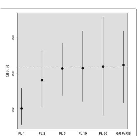
Fig. 3Log-growth model - EM intermediate quantity. Estimation of the EM intermediate quantityQ(θ,θ)using the fixed lag (FL) technique for five different lags, and the GRand PaRIS algorithm using 200 replicates. The whiskers represent the extent of the 95% central values. The dot represents the empirical mean over the 200 replicates. The dotted line shows the reference value, computed using the GRand PaRIS algorithm withN=5000 particles
reference value is then computed as the arithmetic mean of these 30 estimations, and denoted byQ. Figures2and 3display this estimate for an example with one simulated data set. The GRand Paris algorithm is performed using
N = 400 particles in both cases, the fixed lag technique
usingN = 1600 so that both estimations require
simi-lar computational times, resulting a fair comparison. On a personal computer1, for the parameters mentioned above, it takes around 25 s to perform each E step.
5.1 The SINE model
The performance of the GRand PaRIS algorithm are first highlighted using the SINE model, where(Xt)t≥0is
sup-posed to be the solution to
dXt=sin(Xt−μ)dt+dWt, X0=x0. (15)
This simple model has no explicit transition density, however, GPEs may be computed by simulating Brownian bridges. The process solution to (15) is observed regularly at times t0 = 0,. . .,t100 = 50 through the observation
process(Yk)0≤k≤100:
Yk =Xk+εk,
where the (εk)0≤k≤100are i.i.d.N0,σobs2 , the resulting set of model parameters isθ = (μ,σobs). In the example
In the case of the SINE model, the estimatorqkdefined
by Eq. (14) satisfies both (10) and (11). The corresponding boundσ+k can be obtained using numerical optimization. If that bound is chosen, the GRand PaRIS algorithm has linear complexity in the number of particles. As an alter-native, it is worth noting here that the boundsσ+k,i, 1 ≤
i≤N, defined by (12) can also be used. This method has a quadratic cost in the number of particles but provides the
optimal bound for the algorithm of Lemma1. This may
reduce significantly the expected time before acceptance, in particular when the time stepkis large. In the experi-ment configuration presented here, both bounds resulted in an equivalent computational time.
This same experiment was reproduced on 100 different simulated data sets. For each simulation s, the empiri-cal absolute relative biasarbs and the empirical absolute
coefficient of variationacvsare computed as
arbs=
m(Qs)−Qs Qs
,
acvs= σ( Qs) m(Qs) ,
where mQs and σQs are the empirical mean and
standard deviation of the sequence Qs1,. . .,Qs200. For each estimation method, the resulting distributions of arb1,. . .,arb100 and acv1,. . .,acv100 are shown in
Figs.4and 5.
The GRand PaRIS algorithm outperforms the fixed-lag methods for any value of the lag as the bias is the lowest (it is already negligible forN = 400) and with a lower
Fig. 4SINE model - bias. Distribution of the empirical absolute relative bias
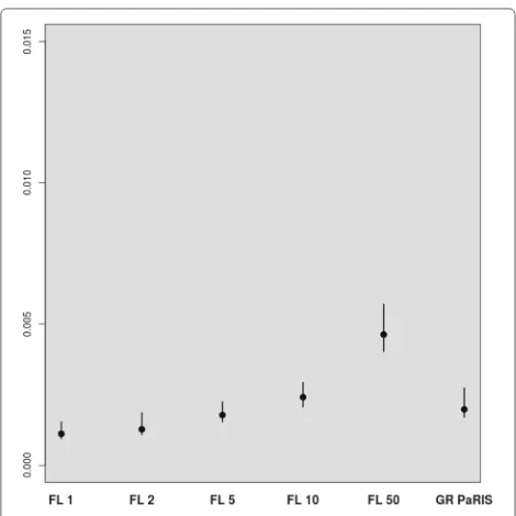
Fig. 5SINE model - variance. Distribution of the empirical absolute coefficient of variation
variance than fixed lag estimates with negligible bias (i.e., in this case, lags larger than 10). Small lags lead to strongly biased estimates for the fixed-lag method, and unbiased estimates are at the cost of a large variance. It is worth noting here that the lag for which the bias is small is model dependent.
Generalized EM procedure The performance of our algorithm is also assessed in the case where θ and the varianceσobs2 are unknown and estimated using a gener-alized EM algorithm. The study is done using a data set
with n = 200 observations simulated with μ = 0
an d σobs2 = 1. The GRand PaRIS algorithm is used
to perform the E step, with the same settings as before forN, N˜, andM. As there is no closed form solution to compute the M step of the EM algorithm and propose new parameter estimates, we use a generalized EM proce-dure: given the current estimationθ(k):=μ(k),σobs(k), the
functionQ·,θ(k)is approximated for 50 new candidates θ1,. . .,θ50chosen by the user. The new estimate is set as
θ(k+1) = argmax
iQ
θi,θ(k)
.
This procedure has the nice property of using the same particle filter and the same retrospective sampling of Lemma1for all candidates, avoiding to repeat this time consuming procedure. The number of candidates and the way to choose them is problem dependent and then left to the user. In our case, we sampled candidates using Gaussian distributions around the current estimateθ(k),
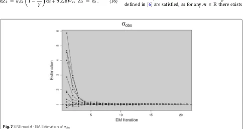
Fig. 6SINE model - EM. Estimation ofμ
illustrate the performance of the estimation for 12 differ-ent initializations of μ (resp. σobs) uniformly chosen in
]−π,π[ (resp. in ] 0, 6[), illustrating a convergence after only a few iterations of the EM procedure.
5.2 Log-growth model
Following [6] and [28], the performance of the proposed algorithm are also illustrated with the log-growth model (Fig.8) defined by
dZt = κZt
1−Zt γ
dt+σZtdWt, Z0 = z0. (16)
In order to use the exact algorithms of [6] and the GPE of [13], we consider (16) after the Lamperti transform, i.e., the process defined byXt = η(Zt), withη(z) : = − log(z)/σ, which satisfies the following SDE:
dXt=
:=α(Xt)
σ
2−
κ
σ+
κ
γ σexp(−σXt)
dt+dWt, X0=x0=η(z0).
(17)
In this case, the conditions of the exact Algorithm 2 defined in [6] are satisfied, as for anym ∈ Rthere exists
Fig. 8Log-growth model - observations. ProcessXsolution to the SDE (balls) and observationsY(circles) at timest0=0,. . .,t100 = 50
Um such that for allx ≥ m, ψ(x) := α2(x) +α(x) ≤
Um. Moreover,ψis lower bounded uniformly byL. Then,
GPE estimators may be computed by simulating the mini-mum of a Brownian bridge, and simulating Bessel bridges conditionally to this minimum, as proposed by [6].
The process solution to (17) is observed regularly at times t0 = 0,. . .,t50 = 100 through the observation
process(Yk)0≤k≤50defined as
Yk =Xk+εk,
where the(εk)0≤k≤50are i.i.d.N
0,σobs2 . The parameters are given by
θ =(κ=0.1,σ =0.1,γ =1000,σobs=2).
In the case of the log-growth model, the estimatorqk(·)
defined by Eq. (14) satisfies (11), leading to a GRand PaRIS algorithm with linear complexity in the number of parti-cles. However, the remarks about the boundσ+k made for the SINE model above still hold in this case. The interme-diate quantity of the EM algorithm is evaluated as for the SINE model, see Figs.3,9, and10.
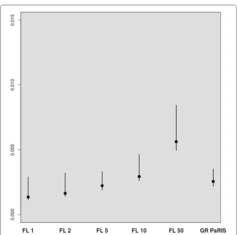
The results for the fixed-lag technique are similar to the ones presented in [27, Figure 1] using the same model. For small lags, the variance of the estimates is small, but the estimation is highly biased. The bias rapidly decreases as the lag increases, together with a great increase of vari-ance. Again, the GRand PaRIS algorithm outperforms the fixed lag smoother as it shows a similar (vanishing) bias as the fixed lag for the largest lag and a smaller variance than the fixed lags estimates with negligible bias.
Fig. 9Log-growth model - bias. Distribution of the empirical absolute relative bias
Note that in this case, the Lamperti transform to obtain a diffusion with a unitary diffusion term depends on σ. The process(Xt)t≥0is a function ofσ and is not directly
observed ifσ is unknown, which prevents a direct use of an EM algorithm to estimateσ. Following [6, Section 8.2], this may be overcome with a two-step transformation of the process(Zt)t≥0.
6 Conclusions
This paper presents a new online SMC smoother for partially observed differential equations. This algorithm relies on an acceptance-rejection procedure inspired from the recent PaRIS algorithm. The main result of the arti-cle for practical applications is that the mechanism of this procedure remains valid when the transition density is approximated by a an unbiased positive estimator. The proposed procedure therefore extends the PaRIS algo-rithm to HMMs whose transition density is unknown and can be unbiasedly approximated. The GRand PaRIS algo-rithm outperforms the existing fixed lag smoother for POD processes of [27], as it does not introduce any intrin-sic and non-vanishing bias. In addition, numerical sim-ulations highlight a better variance using data from two different models. It can be implemented for the class of models for which exact algorithms of [6] are valid, with a linear complexity inNin the best cases, or at worse inN2.
Endnote
1(i7-6600U CPU @ 2.60GHz)
Appendix
Proofs
Proof of Lemma1Letτbe the first time draws are accepted in the accept-reject mechanism. For all≥1, write
Ak
which concludes the proof.
Proof of Lemma 2The independence is ensured by the mechanism of SMC methods. By (9),
Eωi
Moreover, conditionally toFkN, the probability density function ofξki+1,Iki+1is given by
which concludes the proof.
addition,φ0N is a standard importance sampler estimator
Therefore, by Hoeffding inequality,
PaN−E
On the other hand,
EaNFkN=φkN[ϒk] ,
By the induction assumption,
PEbNFkN
The proof is completed using Lemma3.
Lemma 3Assume that aN, bN, and b are random vari-ables defined on the same probability space such that there exist positive constantsβ, B, C, and M satisfying
(i) |aN/bN| ≤M,P-a.s. andb≥β,P-a.s.,
This work has been developed during a 1-year postdoc funded by Paris-Saclay Center for Data Science.
Authors’ contributions
All the authors have contributed to the conception of the algorithms, the analysis of the proposed estimator, and to the redaction of the manuscript. PG provided the simulations displayed in the final version. All authors read and approved the final manuscript.
Competing interests
The authors declare that they have no competing interests.
Publisher’s Note
Springer Nature remains neutral with regard to jurisdictional claims in published maps and institutional affiliations.
Author details
1AgroParistech, UMR MIA 518, F-75231, Paris, France.2Laboratoire de
Mathématiques d’Orsay, Univ. Paris-Sud, CNRS, Université Paris-Saclay, 91405 Orsay, France.
Received: 5 March 2017 Accepted: 11 January 2018
References
1. Y Ait-Sahalia, Transition densities for interest rate and other nonlinear diffusions. J. Financ.54, 1361–1395 (1999)
2. Y Ait-Sahalia, Maximum likelihood estimation of discretely sampled diffusions: a closed-form approximation approach. Econometrica.70, 223–262 (2002)
3. Y Ait-Sahalia, Closed-form likelihood expansions for multivariate diffusions. Ann. Stat.36, 906–937 (2008)
4. A Beskos, O Papaspiliopoulos, GO Roberts, Retrospective exact simulation of diffusion sample paths with applications. Bernoulli.12(6), 1077:1098 (2006)
5. A Beskos, O Papaspiliopoulos, GO Roberts, A factorisation of diffusion measure and finite sample path constructions. Methodol. Comput. Appl. Probab.10(1), 85–104 (2008)
6. A Beskos, O Papaspiliopoulos, GO Roberts, P Fearnhead, Exact and computationally efficient likelihood-based estimation for discretely observed diffusion processes (with discusion). J. Roy. Statist. Soc. Ser. B.
68(3), 333–382 (2006)
7. O Cappé, E Moulines, T Rydén,Inference in hidden Markov models. (Springer-Verlag, New York, 2005)
8. P Del Moral, J Jacod, P Protter, The Monte Carlo method for filtering with discrete-time observations. Probab. Theory Relat. Fields.120, 346–368 (2001)
9. AP Dempster, NM Laird, DB Rubin, Maximum likelihood from incomplete data via the EM algorithm. J. Roy. Statist. Soc. B.39(1), 1–38 (1977). (with discussion)
11. A Doucet, S Godsill, C Andrieu, On sequential Monte-Carlo sampling methods for Bayesian filtering. Stat. Comput.10, 197–208 (2000) 12. A Doucet, S Godsill, C Andrieu, On sequential monte-carlo sampling
methods for bayesian filtering. Stat. Comput.10, 197–208 (2000) 13. P Fearnhead, O Papaspiliopoulos, GO Roberts, Particle filters for partially
observed diffusions. J. Roy. Statist. Soc. Ser. B.70(4), 755–777 (2008) 14. P Fearnhead, K Latuszynski, GO Roberts, G Sermaidis, Continuous-time
importance sampling: Monte Carlo methods which avoid time-discretisation error (2017). Technical report
15. P Gloaguen, M-P Étienne, S Le Corff, Stochastic differential equation based on a multimodal potential to model movement data in ecology. To appear in the Journal of the Royal Statistical Society: Series C.http:// onlinelibrary.wiley.com/doi/10.1111/rssc.12251/abstract
16. SJ Godsill, A Doucet, M West, Monte Carlo smoothing for non-linear time series. J. Am. Stat. Assoc.50, 438–449 (2004)
17. N Gordon, D Salmond, AF Smith, Novel approach to
nonlinear/non-Gaussian bayesian state estimation. IEE Proc. F. Radar Sig. Process.140, 107–113 (1993)
18. M Hürzeler, HR Künsch, Monte Carlo approximations for general state-space models. J. Comput. Graph. Stat.7, 175–193 (1998) 19. N Kantas, A Doucet, SS Singh, J Maciejowski, N Chopin, On particle
methods for parameter estimation in state-space models. Stat. Sci.30(3), 328–351 (2015)
20. M Kessler, Estimation of an ergodic diffusion from discrete observations. Scand. J. Stat.24(2), 211–229 (1997)
21. M Kessler, A Lindner, M Sorensen,Statistical methods for stochastic differential equations. (CRC Press, Boca Raton, 2012)
22. G Kitagawa, Monte-Carlo filter and smoother for non-Gaussian nonlinear state space models. J. Comput. Graph. Stat.1, 1–25 (1996)
23. S Le Corff, G Fort, Convergence of a particle-based approximation of the block online Expectation Maximization algorithm. ACM Trans. Model. Comput. Simul.23(1), 2 (2013)
24. S Le Corff, G Fort, Online expectation maximization based algorithms for inference in hidden Markov models. Electron. J. Stat.7, 763–792 (2013) 25. C Li, Maximum-likelihood estimation for diffusion processes via
closed-form density expansions. Ann. Stat.41(3), 1350–1380 (2013) 26. J Olsson, O Cappe, R Douc, E Moulines, Sequential monte carlo
smoothing with application to parameter estimation in nonlinear state space models. Bernoulli.14(1), 155–179 (2008)
27. J Olsson, J Strojby, Particle-based likelihood inference in partially observed diffusion processes using generalised Poisson estimators. Electron. J. Stat.5, 1090–1122 (2011)
28. J Olsson, J Westerborn, Efficient particle-based online smoothing in general hidden Markov models: the PaRIS algorithm. Bernoulli.3, 1951–1996 (2017)
29. T Ozaki, A bridge between nonlinear time series models and nonlinear stochastic dynamical systems: a local linearization approach. Stat. Sin.2, 1130–135 (1992)
30. MK Pitt, N Shephard, Filtering via simulation: Auxiliary particle filters. J. Am. Stat. Assoc.94(446), 590–599 (1999)
31. G Poyiadjis, A Doucet, SS Singh, Particle approximations of the score and observed information matrix in state space models with application to parameter estimation. Biometrika.98, 65–80 (2011)
32. I Shoji, T Ozaki, Estimation for nonlinear stochastic differential equations by a local linearization method 1. Stoch. Anal. Appl.16(4), 733–752 (1998) 33. M Uchida, N Yoshida, Adaptive estimation of an ergodic diffusion process based on sampled data. Stoch. Process. Appl.122(8), 2885–2924 (2012) 34. W Wagner, Unbiased Monte Carlo estimators for functionals of weak