Maximum likelihood parameter estimation for latent variable models using sequential Monte Carlo

University of Warwick institutional repository: http://go.warwick.ac.uk/wrap

This paper is made available online in accordance with

publisher policies. Please scroll down to view the document

itself. Please refer to the repository record for this item and our

policy information available from the repository home page for

further information.

To see the final version of this paper please visit the publisher’s website.

Access to the published version may require a subscription.

Author(s): Johansen, A; Doucet, A. and Davy, M.

Article Title: Maximum Likelihood Parameter Estimation for Latent

Variable Models Using Sequential Monte Carlo

Year of publication: 2006

Link to published article:

http://dx.doi.org/10.1109/SSP.2007.4301224

Publisher statement:

© 2006 IEEE. Personal use of this material is

permitted. Permission from IEEE must be obtained for all other uses, in

any current or future media, including reprinting/republishing this

material for advertising or promotional purposes, creating new

MAXIMUM LIKELIHOOD PARAMETER ESTIMATION FOR LATENT VARIABLE MODELS

USING SEQUENTIAL MONTE CARLO

Adam Johansen,

_{Arnaud Doucet}

_{and Manuel Davy}

1 - University of Cambridge Department of Engineering, Trumpington Street, Cambridge, CB2 1PZ, UK 2 - Department of Statistics & Department of Computer Science, University of British Columbia, Vancouver, Canada

3 - LAGIS UMR 8146, BP 48, Cit´e scientifique, 59651 Villeneuve d’Ascq Cedex, France

ABSTRACT

We present a sequential Monte Carlo (SMC) method for maximum likelihood (ML) parameter estimation in latent variable models. Stan-dard methods rely on gradient algorithms such as the Expectation-Maximization (EM) algorithm and its Monte Carlo variants. Our approach is different and motivated by similar considerations to sim-ulated annealing (SA); that is we propose to sample from a sequence of artificial distributions whose support concentrates itself on the set of ML estimates. To achieve this we use SMC methods. We con-clude by presenting simulation results on a toy problem and a non-linear non-Gaussian time series model.

1. INTRODUCTION

1.1. Problem Formulation

The situation in which we are interested in is that in which one has some likelihood functionp(y, z|θ)in which(y, z) ∈ Y × Z for observed datayand latent variables (often called “hidden data”),z. Although this joint likelihood is known, aszis not observed, the

marginal likelihood

p(y|θ) =

Z

p(y, z|θ)dz (1)

is the quantity of interest, and as this integral is generally not tractable, it is not straightforward to maximise it with respect to the parameters to obtain the (marginal) maximum likelihood (ML) estimator:

ˆ

θM L_{= argmax} θ∈Θ

p(y|θ). (2)

1.2. Previous Approaches

When the marginal likelihoodp(y|θ)can be evaluated, the classical approach to problems of this sort is the EM algorithm [1], which is a numerically well-behaved gradient-based algorithm. For complex models,p(y|θ) cannot be computed analytically and typically the expectation step of the EM algorithm cannot be performed in closed-form either. In such scenarios, Monte Carlo variants of EM have been proposed – including stochastic EM (SEM), Monte Carlo EM (MCEM) and stochastic approximation EM (SAEM). See [2] for a comparative summary of these approaches. Note that all of these (stochastic) gradient-based approaches are susceptible to trapping in local modes.

An alternative approach related to SA is to build a sequence of distributions which concentrates itself on the set of the required es-timate. Letp(θ)be an instrumental prior distribution whose support

includes the ML estimate then the distributions

pM Lγ (θ|y)∝p(θ)p(y|θ) γ

concentrate themselves on the set of ML estimates as γ → ∞. Indeed asymptotically the contribution from this instrumental prior vanishes. The termp(θ)is here only present to ensure that the distri-butions˘pM L

γ (θ|y)

¯

are integrable – it may be omitted in those in-stances in which this is already the case. To sample from these distri-butions, one would like to use Markov chain Monte Carlo (MCMC) methods. Unfortunately, this is impossible wheneverp(y|θ)is not known pointwise up to a normalizing constant.

To circumvent this problem, it has been proposed in [3] (in a Maximum a Posteriori, rather than ML, setting) to build a sequence of artificial distributions known, up to a normalizing constant, which admit as a marginal distribution the target distributionpM L

γ (θ|y)for an integer powerγ greater than one. A similar scheme was subse-quently been proposed by [4, 5] in the ML setting. This is achieved by simulating a number of replicates of the missing data where one defines

pγ(θ, z1:γ|y)∝p(θ) γ

Y

i=1

p(y, zi|θ) (3)

withzi:j= (zi, ..., zj). Indeed it is easy to check that

Z

· · ·

Z

pγ(θ, z1:γ|y)dz1:γ=pM Lγ (θ|y).

The approach of [3] is to construct an inhomogeneous Markov chain which produces samples from a sequence of such distributions for increasing values ofγ. Just as in SA, this concentrates the mass on

the set of global maxima ofp(y|θ)asγbecomes large. Another ap-proach proposed by [4] is to construct a homogeneous Markov chain whose invariant distribution corresponds to such a distribution for a predetermined value ofγ. It can be theoretically established that these methods converge asymptotically towards the set of estimates of interest ifγ grows slowly enough to∞. However in practice, these approach suffer from several weaknesses. First, they allows only integer values forγ. Second, unless a very slow annealing schedule is used, the MCMC chain tends to become trapped in local modes.

sam-pling and resamsam-pling mechanisms. The population of samples em-ployed by our method makes it much less prone to trapping in lo-cal maxima, and the framework naturally allows for the introduction of bridging densities between target distributions, say,pγ(θ, z1:γ|y) andpγ+1(θ, z1:γ+1|y) for an integerγ.At first glance, the

algo-rithm appears very close to mutation-selection schemes employed in the genetic algorithms literature. However, there are two major dif-ferences with these algorithms. First, they require the function be-ing maximized to be known pointwise, whereas we do not. Second, convergence results for our method follow straightforwardly from general results on Feynman-Kac flows [6].

2. AN SMC SAMPLER APPROACH

2.1. Background

The SMC samplers framework of [7] is a very general method for obtaining a set of samples from a sequence of distributions which can exist on the same or different spaces. This is a generalisation of the standard SMC method (commonly referred to as particle fil-tering and summarised by [8]) in which the target distribution exists on a space of strictly increasing dimension and no mechanism exists for updating the estimates of the state at earlier times after receiv-ing new data. It is not possible to give a thorough exposition of the SMC samplers approach here, but we will try to include sufficient detail for our purposes. We remark that convergence results, includ-ing a central limit theorem, for the particle estimates obtained by this method are available (indeed, these are applications of standard results on Feynman-Kac flows [6]) and are contained in [7].

Given a sequence of distributions(πt)t≥1on a sequence of

mea-surable spaces (Et,E)t≥1 from which we wish to obtain sets of

weighted samples, we construct a sequence of distributions on a se-quence of spaces of increasing dimension which admit the distribu-tions of interest as marginals, by defining:

e

πt(x1:t) =πt(xt)

1 Y

s=t−1

Ls(xs+1, xs)

whereLs is an arbitrary Markov kernel from spaceEs+1 to Es (these act, in some sense, backwards in time). It is clear that stan-dard SMC methods can now be applied on this space, by propagating samples forward from one distribution to the next according to a se-quence of Markov kernels,(Kt)t≥2, and correcting for the

discrep-ancy between the proposal and the target distribution by importance sampling. As always it is important to ensure that a significant frac-tion of the particle set have non-negligible weights. The effective sample size (ESS), introduced by [9], is an approximation obtained by Taylor expansion of a quantity which describes the effective num-ber of iid samples to which the set corresponds. The ESS is defined asESS =hPN

i=1W

(i)−2i−1 _wheren_W(i)o_{are the normalized}

weights. This approximation, of course, fails if the particle set does not accurately represent the support of the distribution of interest. Resampling should be carried out after any iteration which causes the ESS to fall below a reasonable threshold (typically around half of the total number of particles), to prevent the sample becoming de-generate with a small number of samples having very large weights. The rapidly increasing dimension raises the concern that the variance of the importance weights will be extremely high. It can be shown (again, see [7]) that the optimal form for the Markov kernels

Ls– in the sense that they minimise the variance of the importance weights if resampling occurs at every time step – depends upon the

distributions of interest and the importance sampling proposal ker-nelsKtin the following way:

Loptt (xt+1, xt) =

πt(xt)Kt+1(xt, xt+1) R

πt(x)Kt+1(x, xt+1)dx (4)

In practice it is important to choose a sequence of kernels which are as close to the optimal case as possible to prevent the variance of the importance weights from becoming extremely large.

2.2. SMC Samplers for Parameter Estimation

We will consider the use of the sampling methodology described in the previous section for marginal ML estimation – noting that the method can be easily adapted to Bayesian marginal Maximum a Pos-teriori setting by considering a slightly different sequence of target distributions. The target distribution which we propose as generally admissible for this task, although any distribution from which an efficient sampler can be constructed which admit marginals of the desired form would be equally acceptable, is

πt(θ, z1:dγte|y)∝p(θ)

bγ_Ytc

i=1

p(y, zi|θ)p(y, zdγte|θ)

γt−bγtc

wherebγtcdenotes the largest integer not greater thanγtanddγte the smallest integer not less thanγt. This final term allows us to in-troduce sequence with non-integer elements, whilst having the same form as (3). Clearly, we haveπt(θ, z1:dγte|y) =pγt(θ, z1:γt|y)for

any integerγt.Again, an increasing sequence(γt)t≥1 is required,

corresponding in some sense to the annealing schedule of SA. To simplify notation we will denoteZ_t,(i_1:)_dγ

te – the values ofz1:dγte

simulated at timetfor theith particle – byZt(i).Algorithm 1 de-scribes the general framework which we propose.

Algorithm 1: The General Framework Initialisation, t=1:

Sample,n“θ(₁i), Z₁(i)”oN

i=1independently fromν(·)

Calculate importance weightsW₁(i)∝ π1(θ1(i),Z (i) 1 ) ν(θ₁(i),Z₁(i))

If ESS<Threshold, resample. At timet >1:

Sample,n“θ(ti), Z

(i)

t

”oN

i=1such that

∀1≤i≤N:“θ(ti), Z

(i)

t

”

∼Kt

““

θ(_t−i)₁, Z_t−(i)₁”,·” Calculate importance weights

W_t(i) W_t−(i)₁ ∝

πt(θ(ti),Z

(i)

t )Lt−1 ““

θ(_ti),Z_t(i)”,“θ(_t−i)₁,Z(_t−i)₁”” πt−1(θ(_t−i)₁,Z_t−(i)₁)Kt

““

θ(_t−i)₁,Z(_t−i)₁”,“θ(_ti),Z_t(i)”” If ESS<Threshold, resample.

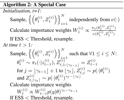
Algorithm 2: A Special Case Initialisation, t=1:

Sample,n“θ(₁i), Z₁(i)”oN

i=1independently fromν(·)

Calculate importance weightsW₁(i)∝π1(θ₁(i),Z₁(i))

ν(θ₁(i),Z₁(i))

If ESS<Threshold, resample.

At timet >1:

Sample,n“θ(ti), Z

(i)

t

”oN

i=1such that∀1≤i≤N: θ(ti)∼πt(·|z(t−i)1),Z

(i)

t,1:bγt−1c=Z

(i)

t−1

forj=bγt−1c+ 1tobγtc,Z(t,ji)∼p(·|θ

(i)

t ) andZ_t,dγ(i)

te∼p(·|θ

(i)

t ) γt−bγtc

Calculate importance weights

Wt(i)∝W

(i)

t−1p(y|θ)γt−γt−1

If ESS<Threshold, resample.

Finally, we present a generic form of the algorithm which can be applied to a broad class of problems, although it will often be less efficient to use this generic formulation than to construct a dedicated sampler for a particular class of problems. We assume that a col-lection of Markov kernels(Kt)t≥1with invariant distributions

cor-responding to(πt)t≥1is available, and using these as a component

of the proposal kernels allows the evaluation of the optimal auxil-iary kernel. We assume that good importance distributions for the conditional probability of the variables being marginalised can be sampled from and evaluated,q(·|θ), and that if the annealing

sched-ule is to include non-integer inverse temperatures, then we have ap-propriate importance distributions for distributions proportional to

p(z|θ)α_{, α∈(0,1), which we denoteq}

α(z|θ). We remark that this is not the most general possible approach, but is one which should work acceptably for a broad class of problems.

Algorithm 3: A Generic Case Initialisation, t=1:

Sample,n“θ(₁i), Z₁(i)”oN

i=1independently fromν(·)

Calculate importance weightsWt(i)∝

π1(θ1(i),Z (i) 1 ) ν(θ₁(i),Z₁(i))

If ESS<Threshold, resample. At timet >1:

Sample,n“θ(ti), Z

(i)

t

”oN

i=1such that∀1≤i≤N: “

θt(i), Z

(i)

t,1:bγt−1c

”

∼ Kt−1

“

θ_t−(i)₁, Z_t−(i)₁;·” forj=bγt−1c+ 1tobγtc,Z(t,ji)∼q(·|θ

(i)

t ) andZ_t,dγ(i)

te∼qγt−bγtc(·|θ

(i)

t ) Calculate importance weights

W_t(i) W_t−(i)₁ ∝

bγ_Qtc

j=bγt−1c+1

p(y,Z(_ji)|θ(i)_)p(y,Z(i)

dγte|θ

(i)₎γt−bγtc

q(Z_j(i)|θ(i)_)q

γt−b_γtc(Zγt(i)|θ(i)

If ESS<Threshold, resample.

3. EXAMPLES AND RESULTS

3.1. Toy Example

We consider first a toy example in one dimension. We borrow ex-ample 1 of [5] for this purpose. The model consists of a student

t-distribution of unknown location parameterθwith0.025degrees of freedom. Four observations are available,y = (−20,1,2,3). The logarithm of the marginal likelihood in this instance is given by:

logp(y|θ) =−0.525

4 X

i=1

log`0.05 + (yi−θ)2

´

N T Mean Std. Dev. Min Max

50 15 1.992 0.014 1.95 2.03

100 15 1.997 0.013 1.97 2.04

20 30 1.958 0.177 1.09 2.04

50 30 1.997 0.008 1.98 2.01

100 30 1.997 0.007 1.98 2.01

20 60 1.998 0.015 1.91 2.02

50 60 1.997 0.005 1.99 2.01

Table 1. Simulation results for the toy problem. Each line sum-marises 50 simulations withN particles and final temperature T. Only one simulation failed to find the correct mode.

which is not susceptible to analytic maximisation. However, global maximum is known to be located at1.997, and local maxima exist at {−19.993,1.086,2.906}. We can complete this model by consid-ering the studentt-distribution as a scale-mixture of Gaussians and associating a latent variance parameterZi with each observation. The log likelihood is then:

logp(y, z|θ) =−

4 X

i=1 ˆ

0.475 logzi+ 0.025zi+ 0.5zi(yi−θ)2

˜

In the interest of simplicity, we make use of a linear temperature scale,γt = t, which takes only integer values. As we are able to evaluate the marginal likelihood function pointwise, and can sample from the conditional distributions

πt(z1:γt|θ, y) =

γt Y i=1 Ga „ zi ˛ ˛ ˛

˛0.525,0.025 +(yi−θ) 2

2

«

(5)

πt(θ|z1:γt)∝ N

“

θ˛˛_˛µ(tθ),Σ

(θ)

t

”

(6)

where the parameters

Σ(tθ)=

" _t X i=1 4 X j=1 zi,j

#−1

=

"

1/Σ(_t−θ)₁+

4 X

j=1 zt,j

#−1

(7)

µ(tθ)= Σ

(θ)

t t

X

i=1

yTzi = Σ(tµ)

“ µ(t−θ)1/Σ

(θ)

t−1+y

T

zt

”

(8)

may be obtained recursively. Consequently, we can make use of algorithm 2 to solve this problem. We use an instrumental uni-form[−50,50]prior distribution overθ. Some simulation results

are given in table 1. The estimate is taken to be the first moment of the empirical distribution induced by the final particle ensemble; this may be justified by the asymptotic (in the inverse temperature) normality of the target distribution (see, for example, [2, p. 203]).

3.2. Stochastic Volatility

We take this more complex example from [4]. We consider the fol-lowing model:

Zi=α+δZi−1+σuui Z1∼ N

` µ0, σ02

´

(9)

Yi= exp

„ Zi

2

«

i (10)

-1.5 -1 -0.5 0 0.5 1

0 0.5 1 1.5 2 2.5 3 3.5 4

Particle System Estimates

Inverse Temperature Convergence of the Algorithm

α δ σ

Fig. 1. Parameter estimates as a function of the inverse temperature.

available only as a high dimensional integral over the latent vari-ables,Zand this integral cannot be computed.

In this case we are unable to use algorithm 2, and employ a vari-ant of algorithm 3. The serial nature of the observation sequence suggests introducing blocks of the latent variable at each time, rather than replicating the entire set at each iteration. This is motivated by the same considerations as the previously discussed sequence of dis-tributions, but makes use of the structure of this particular model. Thus, at timet, given a set ofMobservations, we have a sample of M γtvolatilities,bγtccomplete sets andM(γt− bγtc)which com-prise a partial estimate of another replicate. That is, we use target distributions of this form:

pt(α, δ, σ, zt)∝p(α, δ, σ) bγ_Ytc

i=1

p(y, zt,i|α, δ, σ)

×p“y1:M(γt−bγtc), z

1:M(γt−bγtc)

t,i

˛ ˛

˛α, δ, σ”,

wherez1:M(γt−bγtc)

t,i denotes the firstγt− bγtcvolatilities of theith replicate at iterationt.

Making use of diffuse conjugate prior distributions1 _forθ en-sures that the prior distributions are rapidly “forgotten”, leading to a maximum likelihood estimate. Our sampling strategy at each time is to sample (α, δ) from their joint conditional distribution, then to sampleσfrom a Gibbs sampling kernel and to propose block-based

Metropolis-Hastings moves for the existing latent variables (using a Kalman-filter and forward filtering / backward sampling proposal) before proposing new volatilities using the same proposal strategy.

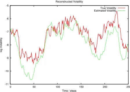
Considering a sequence of 250 observations and a temperature scale which increases in a piecewise linear manner to a temperature of4in340steps, using 250 particles we obtained estimates of the three parameters, by the same mechanism as that used in the toy ex-ample, ofδ= 0.96±0.02,α=−0.25±0.01andσ= 0.31±0.02 where the true values wereδ = 0.95,α=−0.363andσ= 0.26 (suggested by [4] as beingconsistent with empirical estimates for financial equity return time series). Figure 1 shows the estimated parameter values as a function of the number of observations incor-porated. Figure 2 shows the volatility estimated by its posterior mean under the empirical distribution of the final particle set – as the distri-bution overθconverges to a point mass at the maximum likelihood

1_{i.e. uniform over the(}

−1,1)stability domain forδ, standard normal for αand square-root inverse gamma with parametersα= 1,β= 0.1forσ.

-11 -10 -9 -8 -7 -6 -5

0 50 100 150 200 250

log Volatillity

Time / steps Reconstructed Volatility

True Volatility Estimated Volatility

Fig. 2. Estimated volatility (dashed line) obtained using 250 parti-cles and the true volatility (solid line).

value, this amounts to the conditional expectation of the volatility. It is clear that a longer sequence and an annealing schedule which reaches a lower temperature will have a likelihood of very similar functional form with the only difference being that the la-tent variables associated with each observation are replicated, rather than there simply being a greater number of latent variables. Of course longer series provide more information and hence allow bet-ter estimates, indeed, with a sequence of length 1,000 and a final temperature of 1, with just 100 particles, we obtained estimates of

α=−0.40±0.14,σ= 0.28±0.03andδ= 0.95±0.02.

4. REFERENCES

[1] A.P. Dempster, N.M. Laird, and D.B.Rubin, “Maximum likeli-hood from incomplete data vie the EM Algorithm” ,Journal of the Royal Statistical Society, Series B, vol. 39, pp. 2-38, 1977. [2] C.P. Robert, and G. Casella, Monte Carlo Statistical Methods.

New York: Springer-Verlag, second edition,2004.

[3] A. Doucet, S.J. Godsill and C.P. Robert , “Marginal maximum a posteriori estimation using Markov chain Monte Carlo” ,

Statistics and Computing, vol. 12, pp. 77-84, 2002.

[4] E. Jacquier, M. Johannes, and N. Polson , “MCMC maximum likelihood for latent state models” ,Journal of Econometrics, 2005, To Appear.

[5] C. Gaetan, and J.F. Yao , “A multiple-imputation Metropolis version of the EM algorithm” ,Biometrika, vol. 90, no. 3, pp. 643-654, 2003

[6] P. Del Moral,Feynman-Kac Formulae. Genealogical and Inter-acting Particle Approximations, New York: Springer-Verlag, 2004.

[7] P. Del Moral, A. Doucet and A. Jasra, “Sequential Monte Carlo methods for Bayesian computation” (with discussion), in

Bayesian Statistics 8, Oxford University Press, to appear 2006. [8] A. Doucet, J.F.G. de Freitas and N.J. Gordon (eds.),Sequential Monte Carlo Methods in Practice. Statistics for Engineering and Information Science, New York: Springer-Verlag, 2001. [9] A. Kong, J.S. Liu, and W.H. Wong, “Sequential imputations