A Dissertation by
ERIC BENJAMIN BEIER
Submitted to the Office of Graduate Studies of Texas A&M University
in partial fulfillment of the requirements for the degree of DOCTOR OF PHILOSOPHY
December 2011
A Dissertation by
ERIC BENJAMIN BEIER
Submitted to the Office of Graduate Studies of Texas A&M University
in partial fulfillment of the requirements for the degree of DOCTOR OF PHILOSOPHY
Approved by:
Chair of Committee, Lewis Ntaimo Committee Members, Sergiy Butenko
Wilbert Wilhelm Donald Friesen Head of Department, César Malavé
December 2011
ABSTRACT
Subgradient-based Decomposition Methods
for Stochastic Mixed-integer Programs with Special Structures. (December 2011) Eric Benjamin Beier, B.S., Lamar University;
M.E., Texas A&M University
Chair of Advisory Committee: Dr. Lewis Ntaimo
The focus of this dissertation is solution strategies for stochastic mixed-integer programs with special structures. Motivation for the methods comes from the relatively sparse num-ber of algorithms for solving stochastic mixed-integer programs. Two stage models with finite support are assumed throughout. The first contribution introduces the nodal deci-sion framework under private information restrictions. Each node in the framework has control of an optimization model which may include stochastic parameters, and the nodes must coordinate toward a single objective in which a single optimal or close-to-optimal solution is desired. However, because of competitive issues, confidentiality requirements, incompatible database issues, or other complicating factors, no global view of the system is possible.
An iterative methodology called the nodal decomposition-coordination algorithm (NDC) is formally developed in which each entity in the cooperation forms its own nodal deterministic or stochastic program. Lagrangian relaxation and subgradient optimization techniques are used to facilitate negotiation between the nodal decisions in the system with-out any one entity gaining access to the private information from other nodes. A computa-tional study on NDC using supply chain inventory coordination problem instances demon-strates that the new methodology can obtain good solution values without violating private information restrictions. The results also show that the stochastic solutions outperform the corresponding expected value solutions.
The next contribution presents a new algorithm called scenario Fenchel decomposition (SFD) for solving two-stage stochastic mixed 0-1 integer programs with special structure based on scenario decomposition of the problem and Fenchel cutting planes. The algo-rithm combines progressive hedging to restore nonanticipativity of the first-stage solution, and generates Fenchel cutting planes for the LP relaxations of the subproblems to recover integer solutions.
A computational study SFD using instances with multiple knapsack constraint struc-ture is given. Multiple knapsack constrained problems are chosen due to the advantages they provide when generating Fenchel cutting planes. The computational results are promis-ing, and show that SFD is able to find optimal solutions for some problem instances in a short amount of time, and that overall, SFD outperforms the brute force method of solving the DEP.
ACKNOWLEDGMENTS
Much appreciation is due my advisor, Dr. Lewis Ntaimo for his support and advice as I pursued my doctorate. I would also like to thank Dr. Jorge Leon for his part in the Nodal Decomposition-Coordination algorithm. Thank you to the Department of Industrial and Systems Engineering at Texas A&M University for providing financial support and experi-ence in the teaching side of academia. Special thanks go to Judy for always being there to answer my questions and hear my grievances. Finally, thanks to my friends, without whom I could have not made it this far.
Funding for Eric B. Beier: A portion of this research was performed while on appoint-ment as a U.S. Departappoint-ment of Homeland Security (DHS) Fellow under the DHS Schol-arship and Fellowship Program, a program administered by the Oak Ridge Institute for Science and Education (ORISE) for DHS through an interagency agreement with the US Department of Energy (DOE). ORISE is managed by Oak Ridge Associated Universities under DOE contract number DE-AC05-00OR22750. All opinions expressed in this paper are the author’s and do not necessarily reflect the policies and views of DHS, DOE, or ORISE.
TABLE OF CONTENTS
CHAPTER Page
I INTRODUCTION . . . 1
II LITERATURE REVIEW. . . 6
A. Lagrangian Duality and Subgradient Optimization . . . 6
B. Stochastic Linear Programming . . . 10
1. Stage-wise Decomposition . . . 11
2. Scenario-wise Decomposition . . . 14
C. Stochastic Mixed-Integer Programming . . . 18
III NODAL DECOMPOSITION-COORDINATION FOR SMIP WITH PRIVATE INFORMATION . . . 23 A. Introduction . . . 23 B. Related Work . . . 25 C. Problem Formulation . . . 28 D. A Decomposition-Coordination Method . . . 32 E. NDC Algorithm . . . 43
F. A Supply Chain Application . . . 45
1. Linear Cost Functions . . . 51
2. Fixed Charge Cost Functions . . . 52
G. Experiments . . . 54
1. Instance Generation . . . 54
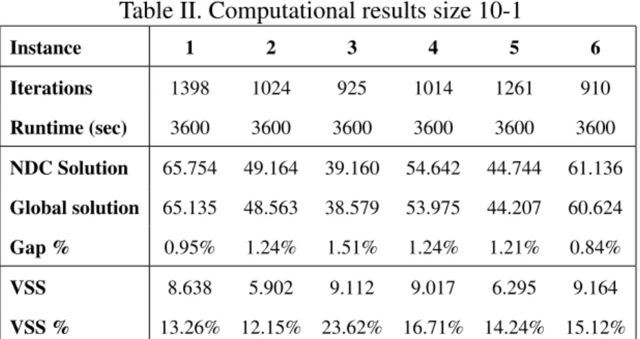
2. Computational Results . . . 57
H. Conclusion . . . 62
IV SCENARIO FENCHEL DECOMPOSITION . . . 64
A. Introduction . . . 64
B. Related Work . . . 66
C. Preliminaries . . . 70
D. Scenario Fenchel Decomposition . . . 74
E. Decomposition Algorithm . . . 79
F. Computational Results . . . 82
1. Design of Experiments . . . 82
CHAPTER Page
G. Conclusion . . . 92
V CONCLUSIONS AND FUTURE WORK . . . 94
REFERENCES . . . 97
APPENDIX A . . . 106
LIST OF TABLES
TABLE Page
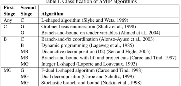
I Classification of SMIP algorithms . . . 19
II Computational results size 10-1 . . . 59
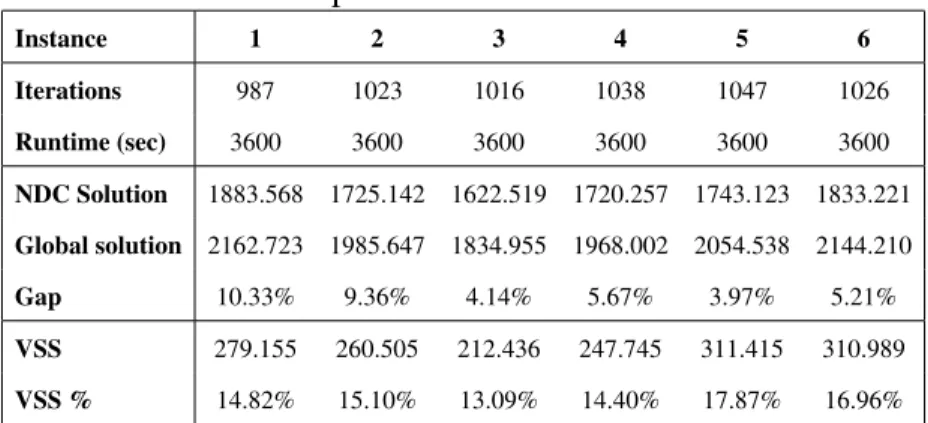
III Computational results size 10-20-1 . . . 59
IV Computational results size 10-15-10-1. . . 60
V Results of test set 1 . . . 84
VI Results of test set 2 . . . 85
VII Results of test set 3 . . . 87
VIII Results of test set 4 . . . 88
IX Additional problem information from test set 1 . . . 107
X Additional problem information from test set 2 . . . 108
XI Additional problem information from test set 3 . . . 109
LIST OF FIGURES
FIGURE Page
1 A Subgradient Optimization Algorithm . . . 9
2 The L-Shaped Algorithm . . . 12
3 The Progressive Hedging Algorithm. . . 18
4 Graphical representation of nodal decision structure. . . 29
5 The Nodal Decomposition-Coordination Algorithm . . . 44
6 Graphical representation of a supply chain . . . 46
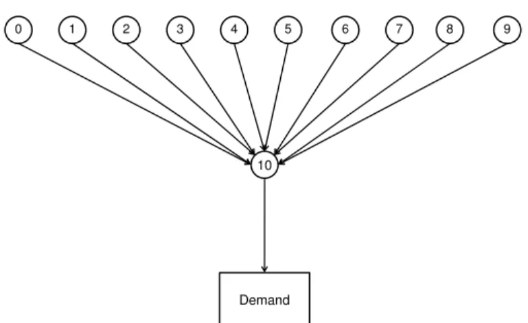
7 Graphical representation of instances sized 10-1 . . . 55
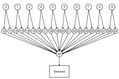
8 Graphical representation of instances sized 10-20-1 . . . 56
9 Graphical representation of instances sized 10-15-10-1 . . . 57
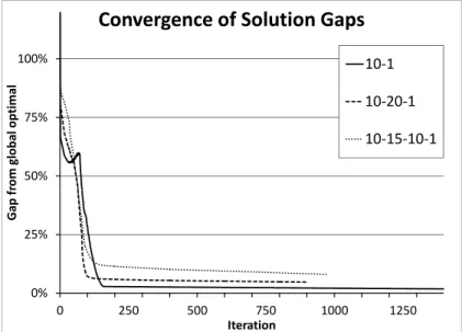
10 Scaled convergence plot of three instances . . . 61
11 The PHA Algorithm . . . 74
12 The Fenchel Cut Generation Subroutine . . . 78
13 The Scenario Fenchel Decomposition Algorithm . . . 79
14 Convergence plot for instance 10.20.25.a . . . 89
15 Convergence plot for instance 20.30.100.a. . . 90
CHAPTER I
INTRODUCTION
Stochastic programming (SP) is a branch of mathematical programming that seeks opti-mal solutions to mathematical optimization problems containing uncertain data. The field of stochastic programming includes two stage stochastic problems, multistage stochastic problems, and problems with chance constraints. This dissertation considers two stage stochastic problems and that is the focus here. Two stage stochastic programs are SPs with two distinct sets of decision variables: a first-stage decision vector representing the “here and now” decisions and a vector of second-stage decision variables, usually calledrecourse decisions, which do not have to be decided upon until after the uncertainty in the problem data has been realized. The general form of a two stage stochastic program is given below:
SP1:Minc>x+E[f(˜ω, x)] s.t. Ax ≥b
x∈Xn1,
(1.1)
whereE[·]denotes the expectation, and for an outcomeωofω˜
f(ω, x) =Minq(ω)>y(ω)
s.t. W(ω)y(ω)≥h(ω)−T(ω)x y(ω)∈Yn2.
(1.2)
In the first stage of SP1 (1.1),xdenotes the vector of first-stage decisions,c∈Rn1 denotes the first-stage objective cost vector,A ∈ Rm1×n1 denotes the first-stage constraint matrix,
b ∈Rm1 denotes the first-stage right-hand side vector, andXn1 denotes special restrictions on the first-stage decisions (such as integral restrictions and upper and lower bounds.) In the second stage of SP1(1.2), f(ω, x) is called the recourse function, y(ω) denotes the recourse decision vector for scenario ω, q(ω) ∈ Rn2 is the second-stage objective cost vector,W(ω) ∈ Rm2×n2 is the recourse matrix,T(ω)∈
Rm2×n1 is the technology matrix,
h(ω)denotes the second-stage right hand side, andYn2 denotes special restrictions on the recourse decisions. In this work, the following assumptions are made on SP1:
(A1) The random variableω˜ follows a discrete distribution with finite supportΩ. (A2) The first-stage feasible set{Ax≥bi, x∈Xn1}is nonempty.
(A3) The second-stage feasible set{W y(ω)≥h(ω)−T(ω)x, y(ω)∈Yn2}is nonempty and bounded for all feasible first-stagex.
Assumption A1 ensures that the formulation is tractable, A2 guarantees the existence of a feasible solution, and A3 is called the “relatively complete recourse” assumption, which guarantees feasibility of the recourse function for all feasiblex. Satisfying A3 can always be accomplished through careful modelling of the problem of interest, such as the imposition of suitably penalized artificial variables to ensure constraint feasibility. Given Assumption A1, let K = |Ω| and assign an ordering k = 1, . . . , K to each realization
ω∈Ω, and letpkdenote the probability of outcomek. Then (1.1) can be restated:
SP2:Minc>x+ K X k=1 pkf(k, x) s.t. Ax≥b x∈Xn1 (1.3)
f(k, x) =Minqk>yk
s.t. Wkyk ≥hk−Tkx yk ∈Yn2.
(1.4)
Formulation (1.4) represents the general form of a two stage stochastic program with finite support, where realization k dictates the data for the matrices from the multivariate random variable. When the setsXn1 andYn2 requirexandykto be continuous variables, SP2 is referred to as a stochastic linear program (SLP). If either set requires all or part of the decision variables to be integer, SP2 is referred to as a stochastic mixed-integer program (SMIP). In order to generate tractable problem formulations, the number of realizations can be limited by restricting how many of these matrices are described by random variables. When the recourse matrix Wk = W, k = 1, . . . , K, the SP is said to havefixed recourse and otherwise it hasrandom recourse. Similarly, SP2 withTk =T, k = 1, . . . , K are said to havefixed technology.
Another classification of SP2 considers feasibility of the recourse function. When
f(x, k) is feasible for any x ∈ R SP2 is said to havecomplete recourse, and the weaker assumption, relatively complete recourse was already introduced as assumption A3. A special case of complete recourse problems is calledsimple recourse. In simple recourse modelsn2 = 2n1 and the recourse matrixWk = [I,−I]∀k(whereI denotes the identity
matrix). Two stage SPs with simple recourse have special properties and are among the simplest SPs to solve.
SP2 can be reformulated as the following deterministic equivalent problem (also re-ferred to as the extensive form):
DEP: Minc>x+ K X k=1 pkqk>yk (1.5a) s.t. Ax≥b (1.5b) Tkx+Wkyk≥hk, k = 1,2, . . . , K (1.5c) x∈X, yk ∈Y, k = 1,2, . . . , K. (1.5d)
DEP can be solved directly using a suitable off the shelf optimizer, providing the optimal solution to (1.3). However, for even moderately dimensioned problems, solving 1.5 directly can be a daunting task, as the number of variables and constraints in (1.5c) and (1.5d) grows exponentially in terms ofK. For this reason, decomposition approaches are usually required in order to find solutions in a reasonable amount of time.
There are two main approaches for decomposing SP2. The first, calledstagewise de-composition, involves relaxing the constraints defining the recourse function and approxi-mating the value of the recourse function by linear approximations. The second approach, calledscenario-wise decomposition uses variable splitting on xallowingK scenario sub-problems to be formulated. One benefit of scenario-wise strategies is that they can generally be applied to multi-stage stochastic programs without much alteration.
In the following chapter, this work is motivated by discussing previous work concern-ing solvconcern-ing SP2. As the theme of this dissertation is focuses on subgradient techniques for solving SMIPs, a brief review of Lagrangian relaxation and subgradient optimization is given. Next, some important theory regarding SLPs is reviewed including a description of the two prevailing decomposition and solution strategies for solving SLP. Finally, some of the major algorithms for solving SMIPs are reviewed.
Chapter III introduces the nodal decomposition-coordination (NDC) algorithm for SMIPs. NDC is motivated by a nodal decision structure where each node represents an
entity with its own optimization model. The nodes in the structure form a group with a common objective, and each node owns its own optimization model whose parameters and decision variables are known only to itself except for a small subset of the variables whose values must be coordinated with some subset of the other nodes. NDC is developed in order to coordinate these decision variables’s values and the algorithm is tested on a set of instances describing a supply chain inventory coordination problem.
Chapter III develops a new algorithm called scenario Fenchel decomposition (SFD) for solving SMIPs based on the progressive hedging algorithm (Rockafellar and Wets, 1991). The algorithm iteratively finds the optimal solution to the LP relaxation of the SMIP using PHA, and then uses Fenchel cutting planes to separate the noninteger point from the convex hull of the (integer) scenario subproblems. The algorithm is tested on a set of randomly generated multidimensional knapsack problems. Finally, Chapter V summa-rizes the contributions of this dissertation and describes the avenues for ongoing and future research.
CHAPTER II
LITERATURE REVIEW
This dissertation focuses subgradient based decomposition methods for stochastic integer programs. This chapter reviews theory necessary for later chapters and summarizes cur-rent state-of-the art approaches for solving stochastic programs. To begin, the concepts of Lagrangian duality and subgradient optimization from linear programming are discussed followed by a review of optimization methods for stochastic programs.
A. Lagrangian Duality and Subgradient Optimization
Lagrangian relaxation techniques are motivated by mathematical programs whose feasible region includes a set of constraints which, if relaxed, would result in problem which is much easier to solve than the original problem. Lagrangian relaxation is a technique commonly used to relax thesecomplicating constraintsin order to have an easier problem to optimize over. Consider the following linear program (LP):
PLP =mincx (2.1a)
s.t. Ax=b (2.1b)
Dx≤d (2.1c)
x≥0. (2.1d)
Assume that constraint (2.1b) is a complicating constraint. Lagrangian relaxation is a well-known method for relaxing complicating constraints from a LP or mixed-integer program (MIP) into the objective. This is accomplished by relaxing the constraint into the objective and penalizing deviations from the constraint. Performing Lagrangian relaxation on (2.1b)
yields the following form: PLR(λ) := min x cx+λ(Ax−b) s.t.Dx≤d x≥0. (2.2)
where the vectorλ is referred to as the Lagrangian multipliers. For a given value of λ,
PLR(λ) (2.2) is known as the Lagrangian relaxation problem. The Lagrangian dual is formed by finding maximal Lagrangian multipliers forPLR(λ)(2.2). The Lagrangian dual has the form
PLD := max
λfreePLR(λ). (2.3)
Due to the presence of a maximization over the the Lagrangian dual problem is sometimes referred to as the max-min dual problem.
The Lagrangian relaxation and Lagrangian dual problems are well studied in the liter-ature. They have many properties that are useful in optimization techniques. (The proofs for these theorems are well documented in the literature and textbooks. See for example Bazaraa et al. (1993).) The first, known as theweak duality theorem for PLR(λ) readily allows for computing a lower bound to the optimal solution ofP.
THEOREM II.1. Given feasible solutionsxtoP andλtoPLR(λ), the following relation-ship holds:
PLR(λ)≤PLP (2.4)
Given the weak duality theorem, the question arises of whether it is possible to guaran-tee that a solution toPLD is optimal forPLP. This is known as thestrong dualitytheorem, and it is well-known to hold for linear programs of the formPLP.
THEOREM II.2. Assume the feasible region of PLP is nonempty and bounded andPLP has a finite optimal and let the optimal values toPLD and PLP bePLD∗ andP
∗
respec-tively. Then
PLD∗ =PLP∗ . (2.5)
Theorem II.2 guarantees that for LPs, an optimum toPLP can be found by solving
PLD. The challenge in solvingPLD is in resolving the outer maximization with the inner minimization. A well-known method for solving the Lagrangian dual is to employ the use of subgradient optimization. In order to apply subgradient optimization to the Lagrangian dual problem, the following concavity theorem is necessary:
THEOREM II.3. Assume the feasible region of PLP is nonempty and bounded andPLP has a finite optimal. ThenPLR(λ)is a piecewise linear concave function ofλ..
For smooth functions, maximization of a concave function can be done by any of sev-eral Newton’s method-based algorithms. However, the piecewise linearity of the function means that PLR(λ) is not everywhere-differentiable over its domain. Fortunately, given concavity, an adaptation of Newton’s method known as subgradient optimization can be used to solvePLD.
DEFINITION II.4. Given concave functiong(λ),ξis called a subgradient ofg atλ¯if
g(λ)≤g(¯λ) +ξ(λ−λ¯)
Showing that the Lagrangian-relaxed constraintAx−bin satisfies the requirement forξis a straightforward application of the theorem. The main idea of a subgradient approach is to use a subgradient in lieu of a gradient in a Newton’s method based approach. A basic subgradient optimization algorithm forPLDis formally stated in Figure 1.
Choosing a step size in Step 1 of the subgradient algorithm can be done in several ways. Theoretically, any divergent series that satisfies P
tµ
t → ∞, µt → 0 ast → ∞ is sufficient, but the convergence rate of such a choice is usually too slow to be used in practice. Instead, the step size µt = ρt U B−PLR(λt)
Subgradient Algorithm
Step 0Select an initial pointλ0. Let iteration countert = 0.
Step 1Letxtdenote the inner minimization solution vector from solvingP
LR(λt). If
Axt−b = 0stop.λtandxtare optimal forPLD. Otherwise, choose step sizeµt >0. Step 2Letλt+1 =λt+µt(Axt−b)and return to Step 1.
Fig. 1. A Subgradient Optimization Algorithm
the optimal solution) is typically chosen in practice, as the rate of convergence is faster, but optimality is not guaranteed. This method is particularly popular when applying La-grangian relaxation to integer programming problems as optimality cannot be guaranteed for general integer programs because Theorem II.2 does not hold, introducing a duality gap between the optimal solution of the Lagrangian dual and the original problem. For details on the choice of a step size in subgradient optimization methods, see Bazaraa et al. (1993) or Nemhauser and Wolsey (1999).
A practical problem is often experienced by researchers employing subgradient opti-mization. If the step size in subsequent iterations is too large, the subgradient step calcu-lation can return solutions that move between a small number of candidates with no im-proving solution. This phenomenon is known as solution oscillation, and can be overcome by the introduction of a regularization term into the objective. The resulting augmented Lagrangian problem is formally stated as
PALR(λ) := min x cx+λ(Ax−b) + ρ 2|Ax−b| 2 s.t.Dx≤d x≥0 λfree, (2.6)
whereρis a user-defined scalar. The quadratic regularization term in the objective seeks to keep the subgradient ascent direction from moving too far from the current xk, thus reducing the liklihood of solution oscillations in an iterative approach. For details on aug-mented Lagrangian approaches see, for example Ruszczy´nski (1986), Rockafellar (1976) or Ruszczy´nski (1995)
B. Stochastic Linear Programming
Next, consider instances of (1.3) in which both the first-stage variables (x) and second-stage variables (y) are continuous. These so called stochastic linear programs (SLP) are among the simplest SPs to solve because wheny∈R, the expected recourse functionE[f(˜ω, xN)] is convex Wets (1974).
The first formulation of a stochastic linear program is generally credited to George Dantzig (Dantzig, 1955), where he introduced the general form of a stochastic linear pro-gram and pointed out the special structure of the formulation. It wasn’t until much later that SLP theory was developed that allowed for efficient decomposition strategies for SLPs. The information contained in this chapter only touches on the basics of stochastic program-ming. For a thorough treatment, see Birge and Louveaux (1997), Ruszczy´nski and Shapiro (2003) or Shapiro et al. (2009).
In general, decomposition methods for two-stage SLPs fall into two categories. The first, discussed in Section 1 is called stage-wise decomposition which adapts theory from
Benders decomposition (Benders, 1962) in order to decompose the problem into a single master problem representing the first-stage decisions and one subproblem for each scenario which contains the second-stage decisions. The second is called stagewise decomposition, which uses variable splitting on the first-stage variables to decompose the problem into one subproblem for each scenario.
1. Stage-wise Decomposition
One of the most well-known decomposition approaches for SLP is Benders decomposition (Benders, 1962). Notice that the dual of 1.5 exhibits a block-angular structure (Dantzig and Wolfe, 1960), which is amenable to Dantzig-Wolfe decomposition (DWD) (Dantzig and Wolfe, 1961). Benders decomposition is a generalized programming method that takes advantage of dual block angular structures and is often considered to be a dual algorithm to DWD. Benders decomposition was first applied to stochastic programs with the develop-ment of the L-shaped algorithm Slyke and Wets (1969). L-shaped methods get their name because of the shape that the first-stage (x) decision vectors make with each set of scenario constraints 1.5c-1.5d in the DEP formulation 1.5.
The L-shaped method is an outer linearization technique which relaxes the second-stage constraints 1.5c-1.5d from DEP and replaces them with linear approximations derived from scenario subproblems. With this in mind, the L-shaped master problem is defined as
MP:Minc>x+θ (2.7a)
s.t. Ax≥b (2.7b)
αtx+θ ≥βtt = 1, . . . , τ (2.7c)
where the optimality cuts 2.7c are derived from dual vectors of the subproblems:
SP(k,xˆ) =Minqk>yk
s.t. Wkyk≥hk−Tkxˆ
yk ∈Yn2.
(2.8)
The L-shaped algorithm is formally stated in Figure 2. L-Shaped Algorithm
Step 0Initialize.τ ←0,ub← ∞,lb← −∞. Solve MP to get solutionxˆ.
Step 1Solve Subproblems. Solve SP(k,xˆ)∀k. Computeπk, the dual vector. Compute
βτ =PKk=1πkhk andατ =PKk=1πkTk Computeub = min{ub, c>x+PK
k=1p
kf(k, x)} Ifubupdated, recordxτ as incumbent.
Step 2Add MP cut and solve. Add cut ατx+θ ≥ βτ to MP. Solve MP, returning solutionsxˆandθˆComputelb=max{lb, c>xˆ+θ}
Step 3 Check termination conditions. If ub −lb < , stop. Report incumbent as
-optimal. Else,τ ←τ + 1. Go to Step 1.
Fig. 2. The L-Shaped Algorithm
Several modifications to the L-shaped algorithm exist. The form given is the classic single cut L-shaped algorithm algorithm. Instead of adding a single cut to MP at each iteration in Step 2, multiple cuts can be added to the MP at each iteration. At each iteration,
the multicut L-shaped algorithm of Birge and Louveaux (1988) adds a cut to the master program for each subproblem k = 1, . . . , K. Theoretically, the benefits of the multicut version over the single cut version are a reduction in the number of L-shaped iterations, but in practice, the larger size of the MP makes choosing the best option problem dependent.
Additionally, if the relatively complete recourse assumption (Assumption (A3)) does not hold, feasibility cuts can be implemented to force the master problem to find feasible first-stage solutions. Consider the situation where a subproblem k is infeasible with the givenxˆsolution in Step 1. In this case, Step 2 can be modified to compute a feasibility cut based on the dual extreme ray, which cuts off thatxˆfrom the feasible region of first-stage decisions. A complete treatment of the L-shaped algorithm can be found in Slyke and Wets (1969).
An important extension to stage-wise decomposition approaches is the regularized L-shaped algorithm Ruszczy´nski (1986). This method augments MP (2.7) with a quadratic term similar to that seen in the augmented Lagrangian relaxation problem. Direct imple-mentations of the L-shaped algorithm can result in a sequence of first-stagexpoints which converge slowly toward the optimum due to the nature of simplex-based approaches for solving the MP. The regularized L-shaped algorithm seeks to eliminate this inefficiency by penalizing new solutions that step too far from the current incumbent.
One final extension of the L-shaped algorithm involves finding solutions whenK be-comes too large for direct application of the L-shaped algorithm. In this case a sampling method such as the stochastic decomposition algorithm Higle and Sen (1991) can be used. The algorithm is an internal sampling method that adds another scenario realization in each iteration to approximate the value of the expected recourse function. Exterior sampling methods, where a new sample of the random variables is drawn at each iteration are referred to as sample average approximation (SAA) methods. For a review of SAA algorithms, see Shapiro (2003).
2. Scenario-wise Decomposition
As discussed, stage-wise decomposition strategies seek to exploit the temporal form of a two stage SMIP. The L-shaped method relaxes the second-stage constraints (1.5c) and (1.5d) and iteratively performs an outer linearization technique, generating the feasibility cuts (2.7c). In scenario-wise decomposition approaches, scenario subproblems are formed by copying the first-stage x decision vector K times using variable splitting, and a La-grangian relaxation approach is typically used to guarantee a feasible solution at termina-tion.
Consider the form of DEP (1.5). The first-stage decision vectorxcan be thought of as “complicating” variables in the sense that if those variables did not exist, the problem would be directly decomposable into a subproblem for each scenariok = 1, . . . , K consisting of only the second-stage decisionsy. Scenario-wise decomposition approaches seek to find optimal solutions by using variable splitting on thexvariables, giving each scenario k its ownxkvariable. This strategy can be thought of as moving the first-stage decisions into the second stage where the probability measure acts on the objective coefficients in the same way as it does theykvariables. Following this approach yields the following form:
VSDEP: Min K X k=1 pkck>xk+qk>yk (2.9a) s.t. Axk ≥b k = 1,2, . . . , K (2.9b) Tkx+Wkyk≥hk, k = 1,2, . . . , K (2.9c) x∈X, yk ∈Y, k = 1,2, . . . , K. (2.9d)
VSDEP decomposes naturally into a subproblem for eachk, but solving the resulting subproblems returns an implementable solution in the general case since thexk solutions returned cannot be translated into a single optimalxsolution to DEP. Requiring equality in
thexksolutions is a concept known asnonanticipativity. Nonanticipativity is the restriction that the first-stage (known as here-and-now) decisions must be decided before the realiza-tion of the random variable is known in the second stage. In the case of scenario-wise decomposition strategies, nonanticipativity must be enforced explicitly with the addition of nonanticipativity constraints. Several forms of nonanticipativity exist. Three forms re-ported in Caroe (1998) are
xk−xk+1 = 0, k = 1, . . . , K −1 xK −x1 = 0 (2.10a) xk− K X s=1 psxs = 0, k = 1, . . . , K (2.10b) xk−xs = 0, k= 1, . . . , K; s∈ {1,2, . . . , K}. (2.10c) The form given in (2.10a) represents a cyclical form, equation (2.10b) gives a form of nonanticpativity in expectation, and (2.10c) chooses a single representative scenario and enforces that value across all scenarios. In this dissertation, the “in expectation” form given in (2.10b) will be used. Adding nonanticipativity constraints of the form (2.10b) to VSDEP (2.9) yields the following deterministic equivalent program.
SWDEP: Min K X k=1 pkck>xk+qk>yk (2.11a) s.t.Axk≥b k = 1,2, . . . , K (2.11b) Tkx+Wkyk ≥hk, k = 1,2, . . . , K (2.11c) xk− K X s=1 psxs = 0, k = 1,2, . . . , K (2.11d) x∈X, yk∈Y, k = 1,2, . . . , K. (2.11e)
An optimal solution to DEP2 is the solution vector(¯x, yk) wherex¯ = PK
k=1p
kxk. Solv-ing SWDEP directly is harder than solvSolv-ing DEP sinceK constraints andKvariables have been added to the problem. However, by using Lagrangian relaxation, SWDEP can be reformulated into a form whose feasible region is decomposable into K subproblems. Performing the variable substitutionx¯ = PK
k=1p
kxk, relaxing the nonanticipativity con-straints (2.11d) via Lagrangian relaxation and introducing the Lagrangian penalty vector
λ={λ1, λ2, . . . , λK}yields the following Lagrangian relaxation formulation:
DEPLR(λ) :Min K X k=1 pkck>xk+qk>yk+λk(xk−x¯) (2.12a) s.t.Axk ≥b, k = 1,2, . . . , K (2.12b) Tkx+Wkyk ≥hk, k = 1,2, . . . , K (2.12c) x∈X, yk ∈Y, k = 1,2, . . . , K. (2.12d)
As with the deterministic case, the Lagrangian dual function becomes DEPLD =Max
For SLPs, subgradient optimization can now be applied to find an optimal solution to SP2 by solving DEPLD.
The progressive hedging algorithm (PHA) presents an augmented Lagrangian ap-proach for solving SP2 (Rockafellar and Wets, 1991). Adding a quadratic regularization term yields the following augmented form:
DEPALR(λ) :Min K X k=1 pkck>xk+qk>yk+λk(xk−x¯) + ρ 2|x k−x|¯2 s.t. Axk ≥b, k = 1,2, . . . , K Tkx+Wkyk≥hk, k = 1,2, . . . , K x∈X, yk ∈Y, k = 1,2, . . . , K. (2.14)
Notice that DEPALRnow has a feasible region that is decomposable intoK subprob-lems. Assuming an iterative procedure (with countert) for updatingλkas discussed in the subgradient optimization review define the PHA subproblem as
SPkP HA(λ) :Minpk[ck>xk+qk>yk+λk(xk−x¯t) + ρkt 2 |x k−x¯ t|2] (2.15a) s.t.Axk ≥b, k = 1,2, . . . , K (2.15b) Tkx+Wkyk ≥hk, k = 1,2, . . . , K (2.15c) x∈X, yk∈Y, k = 1,2, . . . , K, (2.15d)
wherex¯tis calculated by taking the weighted sum of the previous iteration’s solution vector andρkt is chosen to keepxk from moving too far from x¯t from one iteration to the next. Given this formulation, PHA is formally stated in Figure 3.
PHA Algorithm
Step 1: Choose an initial x¯0, step sizes ρk0 and multipliers λk0 and > 0. Set PHA
iteration countert = 0.
Step 2: Solve PkLP(λk)∀k (2.15). Let the solutions be(ˆxkt,yˆkt,λˆkt). Updatex¯t+1 =
K P k=1 pkxˆkt. Step 3: Updateλt+1 =λt+ρk(ˆxkt −x¯t+1). IfPKk=1pk||xˆkt −x¯t||< ,(ˆxkt,yˆtk,λˆkt)is optimal forPk
LP(λk); Report optimal solution variablesxˆkt andyˆtkand corresponding objective
K
P
k=1 Pk
LP(λk). Otherwise incrementt. Go to Step 2.
Fig. 3. The Progressive Hedging Algorithm
C. Stochastic Mixed-Integer Programming
To this point, our treatment of SP has assumed that all variables are continuous. Now con-sider the case when the setsXn1 andYn2 of SP2 (1.3) restrict some or all of the variables to be integer, in which case SP2 becomes a SMIP. SMIPs are among the most difficult op-timization models to solve because the expected recourse function E[f(˜ω, x)] of a SMIP with integer restrictions included in the setYn2 is in general discontinuous and noncovex (Blair and Jeroslow, 1982) (Birge and Louveaux, 1997) (Schultz, 1993). This section sum-marizes some of the important algorithms for SMIP. An extensive review article can be found in Haneveld and van der Vlerk (1999).
exploit specific types of variables in each stage in order to be able to find solutions within a reasonable amount of time. Thus algorithms for SMIP can be classified by the types of variables that they work with. Table I simplifies this classification the major algorithms discussed here. The first two columns describe the types of variables allowed in the algo-rithm: C denotes continuous variables, G denotes pure integer, MG denotes mixed-integer, B denotes pure binary and MP denotes mixed-binary. The third is the name of the algorithm and author.
Table I. Classification of SMIP algorithms
First Second
Stage Stage Algorithm
Any C L-shaped algorithm (Slyke and Wets, 1969)
C G Grobner basis enumeration (Shultz et al., 1998)
G Branch-and-bound on tender variables (Ahmed et al., 2004) B C Branch-and-fix coordination (Alonso-Ayuso et al., 2003)
B Dynamic programming (Lageweg et al., 1985)
MB Disjunctive decomposition (D2) (Sen and Higle, 2005)
MB Branch-and-bound with lift and project cuts (Caroe and Tind, 1997) MG Integer L-shaped (Laporte and Louveaux, 1993)
MG G F-dual L-shaped algorithm (Caroe and Tind, 1998)
MG Dual decomposition(Caroe and Schultz, 1999) MG Stochastic branch-and-bound (Norkin et al., 1998)
Examination of Table I shows that the types of variables in the SMIP dictate the so-lution strategy used. The simplest case of SMIP is whenever the second stage has all continuous variables, in which case the expected recourse function E[f(˜ω, x)] retains its structure and the L-shaped algorithm can be used. However, integer variables in the first stage make convergence of the L-shaped algorithm slow in practice.
While the L-shaped algorithm is not able to solve general SMIP models, many re-searchers adopt the stagewise decomposition framework when developing new algorithms
for solving SMIPs. The integer L-shaped method (Laporte and Louveaux, 1993) merges branch-and-cut with the L-shaped algorithm in order to guarantee convergence of SMIPs with binary first-stage variables and mixed-binary variables in the second stage. The algo-rithm begins by relaxing integrality restrictions and initializing a branch-and-bound tree. The algorithm proceeds by solving the LP relaxation via the L-shaped method and then branching on variables which violate the integrality restrictions. An illustrative example is given, but no computational results are reported.
TheD2 algorithm (Sen and Higle, 2005) has proven very capable of solving SMIPs
with binary first-stage and mixed-binary second-stage. The algorithm solves the first-stage problem as a mixed-binary problem and the linear relaxations of the second-stage sub-problems. The algorithm then uses lift-and-project cuts on the scenario subproblems in order to eventually arrive at an optimal solution. Computational experiments using theD2
algorithm can be found in Ntaimo and Sen (2008).
The F-dual L shaped algorithm of Caroe and Tind (1998) adapts the L-shaped al-gorithm to solve SMIP problems with mixed-integer first-stage variables and pure integer second-stage variables. Instead of using LP-duality ideas to generate optimality cuts, the authors use IP duality theory. The tradeoff is that the master problem becomes nonlinear, and the authors suggest some modifications that make the master problem easier to solve at the expense of optimality.
The next algorithm reviewed is a branch-and-bound algorithm that exploits lift-and-project cuts (Caroe and Tind, 1997). The algorithm iteratively solves the linear relaxation of SMIP and generates lift-and-project cuts Balas et al. (1993) to recover integer solutions. When SMIP has fixed recourse, the authors offer a means by which the cuts generated for one scenario can be translated to another scenario. Theory is developed for SP2 with continuous first-stage variables, then extended to the binary first-stage case by employing branch-and-bound. No computational results are reported.
A dynamic programming approach can be used to solve some instances of SMIP with pure binary first and second-stage variables (Lageweg et al., 1985). The approach requires that the second-stage problem has a very special structure that can be solved using a dy-namic programming approach. Since the set of problems solvable by the algorithm is, the method has not seen wide-spread application, but applications to stochastic scheduling, bin packing and multi-dimensional knapsack problems were demonstrated.
The stochastic branch-and-bound algorithm (Norkin et al., 1998) is able to accommo-date mixed-integer variables in both the first and second stage of a SMIP. This enumerative method iteratively partitions the feasible region, forms estimates of the objective based on those subsets, and then removes subsets that contain no feasible points. The estimates of the objective are statistical estimates and optimality cannot be finitely guaranteed, but sta-tistical estimates of the optimality gap are computed at each iteration. Convergence of the algorithm is illustrated by tests on randomly generated instances from a financial planning application.
Another enumeration based approach uses the Gröbner basis (Shultz et al., 1998). The method divides the first-stage feasible region into a countable number of sections by using properties obtained from the expected recourse function. The authors then make the argument that the optimal solution must be contained in this countable set, and an enumeration algorithm is given to find the optimum from amongst the set.
Ahmed et al. (2004) introduce a branch-and-bound approach on thetender variables. The tender variables are defined as right hand side (hk−Tkx) of the second-stage problem. The authors assume fixed handT matrices for their method. The algorithm reformulates SMIP into a global optimization problem in terms of the tender variables. The reformu-lation results in a semicontinuous function, and the algorithm proceeds by breaking the function into continuous pieces and searching them for the optimum. Computational re-sults compare the performance of the proposed algorithm with other methods from the
literature.
The final two algorithms for SMIP use a scenario-wise decomposition of SP2. The branch-and-fix coordination algorithm (BFC) of Alonso-Ayuso et al. (2003) can be used to solve SMIPs with binary first-stage variables and continuous second-stage variables. The method branches on the first-stage x solutions and uses Dantzig cuts to fix some of the variables which have not been fixed by the branch-and-bound tree. Computational experiments are reported for some large scale models.
A well-known algorithm for solving SMIPs using a scenario-wise decomposition framework is the dual decomposition algorithm (Caroe and Schultz, 1999). The method is applicable to problems with mixed-integer variables in both the first and second stages. The problem is decomposed through the use of nonanticipativity constraints and Lagrangian re-laxation. The Lagrangian dual of the LP-relaxation of the problem is then solved, and branch-and-bound is used in order to recover integer solutions. A computational study demonstrates the effectiveness of the algorithm.
CHAPTER III
NODAL DECOMPOSITION-COORDINATION FOR SMIP WITH PRIVATE INFORMATION
A. Introduction
Traditional optimization problems assume that there exists some omnipotent governing body that has access to all the operational information of the system being examined. This coordinating decision maker can then take all of this information and find a solution that is globally optimal for the system. In reality, many systems are composed of independent bodies that are unable or unwilling to reveal their private information regarding their op-erations to such a decision maker. Thus finding a globally optimal solution when private information restrictions are in place is an important topic in many areas of operations re-search, including supply chain coordination and homeland security. One application where private information is often ignored is in supply chain coordination of inventory and pro-duction schedules. An issue in supply chain management is inventory control, which deals with decisions related to how much inventory to keep at each facility and when to reorder so as to minimize overall inventory ordering and holding costs, service levels, or other relevant objectives.
Problems that arise when attempting global coordination can be very complex even when dealing with a single facility. The difficulty is augmented when expanding to supply chains, and further complicated when considering competitors in the same supply chain, and unwillingness (or practical difficulties) to share critical information. For instance, de-mand rates and transport times are random variables, while inventory holding costs, pro-The notation regarding Lagrangian relaxation in this chapter differs from that used in Chapter II.
duction capacity, operational costs, budgets and lead times are typically private information between competitors. Also, the amount of information that must flow from all firms in the supply chain to the central decision maker can be very large and frequent. It is evident from the literature that private data restrictions in coordinated systems are a common con-cern. However, there still exists a need for methodologies to solve such problems without relaxing this private information requirement and information uncertainty.
This paper introduces nodal decomposition-coordination (NDC) for optimization models with the goal of facilitating global coordination under private information restric-tions and stochastic demand. The approach presented is an iterative methodology, whereby each entity in the cooperation forms its own nodal problem, which can be a mixed-integer program (MIP) or stochastic mixed-integer program (SMIP). Lagrangian relaxation and subgradient optimization techniques are used to facilitate negotiation between the nodal decisions without any one entity gaining access to the private information of other entities. In this coordinated system, optimal or close-to-optimal solutions for the system are desired. This work makes the following contributions to the literature on optimization with private information restrictions: a) stochastic programming model with private information restrictions; b) NDC solution methodology for SMIP with private information restrictions; c) application of the NDC method to supply chain inventory coordination; and d) computa-tional results demonstrating that close-to-optimal solutions can be obtained using the NDC method without compromising private information restrictions. To the best our knowledge, this the first time private information restrictions have been applied to SMIP.
The rest of this paper is organized as follows: In the next section, relevant research from the literature is reviewed. In Section C a model formulation is given for a general problem. In Section D the foundation is developed for the NDC method for the general problem and in Section E the NDC algorithm is presented. Section F introduces a sup-ply chain inventory control model as a special case of the general model and the solution
method is applied. Section G discusses solving the models, presents results and draws conclusions.
B. Related Work
Some algorithms suggesting how to solve optimization problems when global sharing of information is not allowed exist in the literature. Fox et al. (2000) explains some of the emerging strategies in supply chain coordination, which employ agents outside of the chain to coordinate the needs of organizations in the supply chain. The view taken in the paper is one which considers each agent in the supply chain to be its own intelligent software system. The authors suggest several traits that the next generation of agile planning systems should address in order to meet the challenges required. They make the case that such supply chain software must be distributed, dynamic, intelligent, integrated, responsive, reactive, cooperative, interactive, anytime, complete, reconfigurable, general, adaptable, and backwards compatible.
Shehory and Kraus (1998) takes a look at the problem of assigning a group of agents to a group of tasks. They use a greedy heuristic algorithm for the set covering and set partitioning problems to aid in grouping the agents into coalitions to solve the set of tasks to be completed. They demonstrate the effectiveness of their algorithm on a simulation of assigning a group of agents to a set of precedence constrained tasks.
Cruijssen et al. (2007) give a transportation example and explain how some of the in-formation sharing concerns affect that industry. In their paper, they discuss the horizontal cooperation practices in Flanders, Belgium. The study is survey based, and includes re-sponses from 1537 logistic service providers in the Flemish region which asked them to agree or disagree with 16 propositions concerning the implementation and effectiveness of horizontal cooperation. Among the conclusions drawn is that even when customer
infor-mation (which would ordinarily be closely guarded private inforinfor-mation) is required to be shared among competing companies, the potential reduction in costs and increase in profits by cooperating with competing firms is attractive to most firms.
Jeong and Leon (2002a) derive a methodology by which to globally solve MIPs dis-playing a structure that does not allow for some constraints to be globally viewed. The authors term their methodology ‘cooperative interaction via coupling agents’ (CICA). In such a problem structure, different entities in a system where a global optimal value is de-sired are competing for some resource. The method involves using an artificial entity called a ‘coupling agent’ to handle conflict resolution among entities vying for the use of a shared resource. The work in Jeong and Leon (2002a) has been expanded upon in several other papers. In Jeong and Leon (2003) the authors apply their CICA method to coordination of a facility among business competing for use of the resource. In Jeong and Leon (2005) the method is applied to solve the minimum makespan problem when a machine is required in different steps in an assembly line. In Jeong and Leon (2002b) the method is applied to a system where only two resources are available to produce a final product, but multiple firms have a stake in the production line.
An interesting problem where private information is often ignored is in supply chain coordination of inventory and production schedules. A scalable methodology is presented in Chu and Leon (2009). The method involves using Lagrangian relaxation to take care of constraints that would be private to certain firms in the supply chain and appropriate Lagrangian penalty functions are developed to force the method toward a globally optimal solution. However, the solution strategy presented does not take into consideration the stochastic nature of the parameters in the model. In Chu and Leon (2008) this procedure is applied to a deterministic supply chain model. This work develops a new decomposition-coordination method for the stochastic setting and in essence extends the work of Chu and Leon (2009). Further, the application describing supply chain coordination of inventory
and production introduced in Chu and Leon (2009) is used to test the new methodology. Schneeweiss and Zimmer (2004) describe a made to order production line in which co-ordination between entities in the system is maintained through the use of external agents. These external agents shield private information of each node from the other node. Gian-noccaro and Pontrandolfo (2004) use a contract scheme with revenue sharing to coordinate the efforts of the members in the supply chain while maintaining private information. How-ever, such revenue sharing contract schemes have limitations in some industries, as pointed out in Cachon and Lariviere (2005).
Other applications for which finding a globally optimal solution when private infor-mation restrictions are in place exist. An example is in matters of homeland security. Chen et al. (2004) provides a review of relevant areas where information is kept private in a co-operative arrangement. Application areas mentioned include information sharing across jurisdictional bounds, terrorist information collection, modeling and analysis, bioterrorism applications, and border security. The paper proposes the use of current trends in data anal-ysis and information sharing, including system interoperability, data mining, automated event monitoring and visualization.
Phillips Jr. et al. (2002) explains structures where militaries, governments, and civilian companies have to work together in crisis situations, and makes the case that military and government agencies cannot always divulge information to the private sector. The focus of the paper is on coalitions which are formed very quickly in the wake of a large scale crisis such as a natural disaster or terrorist attack. Mendonca (2007) provides a critique of coordination methods used to solve problems in the chaotic and multi-tasked situation that arose in response to the 2001 World Trade Center attack and focuses on developing a set of requirements for computer systems to allow interoperability in future emergency situations. The paper concludes that for a system to be effective in responding to an ex-treme disaster situation it needs to focus on the areas of categorization, search, assembly,
constraint satisfaction, communication, and inference.
There is a limited bank of information in the literature regarding the addition of stochastic data in formulations of supply chain models. In Santoso et al. (2005), the au-thors apply sampling strategies based on the sample average approximation methodology (Shapiro, 2003) to find high quality solutions to two supply chain coordination formula-tions. Alonso-Ayuso et al. (2003) formulates a two stage binary supply chain problem with the objective of maximizing expected profit. The model presents the production topology, plant sizing, product selection, product allocation and vendor selection decisions as 0-1 variables in the first-stage, and a solution strategy based on the Branch-and-Fix Coordina-tion strategy is proposed. Escudero et al. (1999) develops a model for a manufacturing, assembly and distribution supply chain with uncertain demand and prices and uses a dual approach splitting variable scheme to solve the formulation. Petrovic et al. (1999) use the idea of fuzzy sets to handle stochastic parameters in a serial supply chain structure. The next section introduces a general problem formulation for problems fitting the nodal deci-sion structure.
C. Problem Formulation
Consider models with a special nodal decision structure in which each node is responsible for optimally assigning its resources toward the node’s operations. In this framework, the nodal structure faces some degree of uncertainty in the last node of the cooperation. Such a model forms whenever a group of independent entities work together as a corporation or alliance to reach the common goal of obtaining an optimal global solution to a problem under uncertainty. Finding a global solution requires that independent nodal decisions coordinate with other nodes. In this setting, this coordination is represented by a set of resources or decisions called complicating orlinking variables whose allocation must be
coordinated with other nodes in the system. A pair of nodes who share linking variables will be called neighborsand the neighbors of nodeiwill be denotedN(i). In the system, no node is allowed to gain knowledge of the operations (represented in the constraint and objective function parameters) of any of its neighbors or any other nodes in the system.
1
2
6
5
3
4
Uncertainty
6
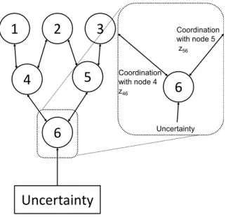
Uncertainty Coordination with node 4 z46 Coordination with node 5 z56Fig. 4. Graphical representation of nodal decision structure
Figure 4 depicts an example nodal structure with 6 nodes. The “Uncertainty” box represents outside influences (exogenous uncertainty) on the system. For example, in the case of a manufacturing setting demand for final product may not be directly controllable by the system, and thus would fall into this category. The exploded view of node 6 at the right emphasizes that there exist linking variables (represented by the double arrow) between the neighboring node pairs 3 and 6 and 5 and 6. The single arrow at the bottom of the node represents that some parameters from outside the system influence the operations of the node.
The nodal decision problem, which takes the form of a two-stage SLP with special private information constraints can now be formulated. Assume the structure describes a
corporation withNnodes, numbered1toN. For the problems which fit into this modelling framework the decision problems for nodes 1 throughN−1take the form of a deterministic MIP and the decision problem for node N takes the form of a SMIP. The vector zi will denote the linking variables at nodei. For example, in Figure 4,z6is a vector consisting of
the variablesz46andz56. The nodal stochastic program with private information (NSP-PI) restrictions can be given as follows:
NSP-PI:Min N X i=1 c>i xi+d>i zi +E[f(˜ω, xN)] (3.1a) s.t. Aixi+Gizi ≥bi i= 1, . . . , N (3.1b) xi ∈Xi, zi ∈Zi i= 1, . . . , N (3.1c) ci, di, Ai, Gi, bi, xi ∈ P(i) i= 1, . . . , N, (3.1d) whereEis the mathematical expectation operator,ω˜ is a multivariate random variable, and for each outcomeω ofω˜, therecoursefunctionf(ω, xN)for nodeN is defined as
f(ω, xN) =MinqN(ω)>yN(ω) (3.2a) s.t. WNyN(ω)≥hN(ω)−TN(ω)xN (3.2b) yN(ω)∈Y (3.2c) qN(ω), WN, TN(ω), VN(ω), hN(ω), yN ∈ P(N). (3.2d) In NSP-PI (3.1),xi ∈ Rn x i and z i ∈ Rn z
i are the first-stage decision vectors for node i, while ci ∈ Rn
x
i anddi ∈ Rnzi are the first-stage cost vectors. Ai ∈ Rm1i×nxi andGi ∈
Rm 1
i×nzi are the first-stage constraints and bi ∈ Rm1i is the first-stage righthand side. The
andzi, respectively, in constraints (3.1c). In constraint (3.1d) the set P(i)imposes private information restrictions on the first-stage problem data for nodei.
In the second-stage (recourse) problem (3.2),yN(ω) ∈ Rn
y
N is the recourse decision
vector for node N and qN(ω) ∈ Rn
y
N is the second-stage cost vector. WN ∈ Rm
2
N×n y N
is the recourse constraint matrix, TN(ω) ∈ Rm 2
N×nxN is the technology constraint matrix, VN(ω)∈ Rm
2
N×nzN is the node linking constraint matrix, andhN(ω)∈Rm2N is the
second-stage righthand side. The set YN imposes possible integer (binary) restrictions on all or some components of yN in constraints (3.1c). Like constraint (3.1c), constraint (3.1d) imposes private information restrictions on the second-stage problem data for nodeN.
In the above modeling framework the key issue is optimizing the first-stage decisions (xi, zi)which have to be made without anticipation of future realizations of{qN(ω), TN(ω),
VN(ω), hN(ω)}. After having decided for (xi, zi) and observed {qN(ω), TN(ω), VN(ω),
hN(ω)}, the remaining decisionsyN(ω)are made in an optimal way. The constraints (3.1d) and (3.2d) are termedprivate information constraints and represent the restriction that the operations taking place in each node of the system remain private to that node. The im-position of this constraint causes the model shown to be impossible to formulate in this explicit form, since no single node nor any overseeing entity is allowed to gather the infor-mation required to formulate the model directly! For this reason, a nodal decomposition-coordination approach that preserves the private information constraints will be necessary in order to generate solutions. The following assumptions are made on NSP-PI:
(A1) The random variableω˜ follows a discrete distribution with finite supportΩ.
(A2) For each node i, the first-stage feasible set {Aixi + Gizi ≥ bi, xi ∈ Xi, zi ∈
Zi, ci, di, Ai, Gi, bi, xi ∈ P(i)}is nonempty.
(A3) For node N, the second-stage feasible set {WNyN(ω) ≥ hN(ω) − TN(ω)xN −
nonempty and bounded for all feasible first-stagexN.
Assumption (A1) is required to make the problem tractable while assumption (A2) is re-quired to guarantee the existence of an optimal solution. Assumption (A3) is the so-called relatively complete recourseassumption in stochastic programming. This assumption can easily be satisfied by modeling the problem with this assumption in mind, or by adding appropriate artificial variables and corresponding induced constraints to the second-stage problem to satisfy relatively complete recourse.
NSP-PI without the private information restrictions falls under two-stage SMIP with recourse, which is still a vibrant area of study (Ruszczy´nski and Shapiro, 2003, e.g.). In that case if the integer restrictions on theyN(ω)’s are relaxed, then the expected recourse functionE[f(˜ω, xN)]is a well-behaved piecewise linear and convex function of xi. Thus Benders decomposition (Benders, 1962) is applicable (Wollmer, 1980). Otherwise, when the second-stage variables involve integrality restrictions,E[f(˜ω, xN)]is lower semicontin-uous with respect to(xN)(Blair and Jeroslow, 1982), and is generally nonconvex (Schultz, 1993). Thus SMIP problems are generally difficult to solve. In this case, in addition to the computational difficulty that stems from SMIP, NSP-PI involves private information restrictions. Thus the problem being addressed here is a much more difficult in general.
D. A Decomposition-Coordination Method
We now propose an iterative nodal decomposition-coordination method for NSP-PI that allows for negotiation between the nodes in the supply chain. As mentioned previously, formulating NSP-PI explicitly for all nodes is not possible due to the private information constraints (3.1d) and (3.2d). Observe that the only decision variables linking two nodes
i and j in NSP-PI are zij, and that this variable affects only nodes i and j. These link-ing variables can be considered as belink-ing ‘complicatlink-ing’ variables in the sense that if each
node’s decision was allowed to disagree with its neighbors, the problem would decompose directly into N subproblems. Similar to Chu and Leon (2009), introduce the following auxiliary variables to facilitate negotiation:
uij: Negotiation variable in nodei’s subproblem denoting nodei’s proposed value to nodej for variablezij (uidenotes the vector ofuij variables.)
vij: Negotiation variable in nodei’s subproblem denoting nodej’s proposed value to nodeifor variablezij (videnotes the vector ofvij variables.)
For a given nodei, substitute the variablesuij in (3.1) forzij to represent the node’s complicating decision vector with its neighborj, andvijforzij to denote the corresponding decision vector for neighborj. In order to solve the original problem,uij andvij must be equal for each pair of neighboring nodes iandj. To achieve this, one can implement one of several equivalent negotiation constraints. Two are given below:
uij = ¯zij (3.3a)
uij −vij = 0. (3.3b)
The first form (3.3a) forces equality of the negotiation variable in each subproblem to some third value. The constraint works becauseuij is found in the subproblem of each pair of neighboring nodes. In practice, the valuez¯ij can be set by taking the average 12(uij+vij), which is the approach implemented here. The second constraint set is a constraint that directly forces each pair of coordination variables to agree.
Using these new variables and equation, a variable splitting technique can be applied to (3.1) to getN decoupled subproblems. The resulting subproblem for nodei6=N becomes:
NSP-PI2(i) :Minc>i xi+d>i ui (3.4a)
s.t. Aixi +Giui ≥bi (3.4b)
uij = ¯zij j ∈ N(i) (3.4c)
xi ∈Xi, ui ∈Zi, vi ∈Zi (3.4d)
ci, di, Ai, Gi, bi, xi ∈ P(i) (3.4e) and, for node N:
NSP-PI2(N) :Minc>NxN +dN>uN +E[f(˜ω, xN)] (3.5a)
s.t. ANxN +GNuN ≥bN (3.5b)
uij = ¯zij j ∈ N(i) (3.5c)
xN ∈XN, uN ∈ZN, vN ∈ZN (3.5d)
cN, dN, AN, GN, bN, xN ∈ P(N) (3.5e) where, for a particular realizationω ∈ω˜:
f(ω, xN) =MinqN(ω)>yN(ω) (3.6a) s.t. WNyN(ω)≥hN(ω)−TN(ω)xN (3.6b)
yN(ω)∈Y (3.6c)
qN(ω), WN, TN(ω), VN(ω), yN(ω)∈ P(N). (3.6d) Lagrangian relaxation can now be applied to relax constraints (3.4c) into the objec-tive. By choosing appropriate penalty parameters, negotiation between nodesi andj can
be achieved. The solution procedure will require solving two subproblems at each node: a coordinated subproblem which takes into account the propositions made by node (i)’s neighbors by penalizing deviations fromz¯ij in node(i)’s decisions, and anon-coordinated subproblem that requires that the (i)’s neighbors receive exactly the compromise target valuez¯ij. In each iteration all nodes will first solve their non-coordinated problems. Then, each node will solve their coordinated problem and pass their requests for order and de-livery quantities to their neighbors for the next iteration. The procedure will be further explained after these two subproblems are defined.
For each node i define the non-coordinated subproblem (NCP) as the optimization problem specific to the node that is required to satisfy exactly the compromise value. For consistency and convenience whenever a variable is treated as data, determined based on the node(i)’s neighbors, it will be designated as such with the ˆ notation. Then substituting forz¯ij in NSP-PI2(i) 3.4 for node iresults in the following non-coordinated subproblem for node16=N:
NCP(i) :Minc>i xi+d>i zˆi (3.7a) s.t. Aixi+Gizˆi ≥bi (3.7b)
xi ∈Xi (3.7c)
ci, di, Ai, Gi, xi ∈ P(i) (3.7d) and for nodeN:
NCP(N) :Minc>NxN +dN>zˆN +E[f(˜ω, xN)] (3.8a) s.t. ANxN +GNzˆN ≥bN (3.8b)
xN ∈XN (3.8c)
cN, dN, AN, GN, xN ∈ P(i) (3.8d) An issue with feasibility can arise when solving NCP(i). Infeasibility can occur in cases where the compromise value resulting from node(i)’s neighbor’s requests generates value for the linking variables which causes NCP(i)to become infeasible. One method to maintain feasibility is to add an artificial variable to 3.7b and penalize it in the objective. This method is adopted later in the computational study section of this paper.
Next thecoordinated subproblem(CP) needs to be defined. Contrary to NCP, the coor-dinated problem for nodeiallows for deviations from the compromise quantities negotiated with its neighboring nodes (j ∈ N(i)) in the cooperation. An augmented Lagrangian ob-jective function is adopted for CP. Let µij denote the Lagrangian multipliers associated with the negotiation constraints (3.3a) in CP for node(i)’s neighbors For eachj ∈ N(i), let the Lagrangian relaxed constraints be defined as
Note that in the equationzˆij is known (data) based on calculations from node(i)’s neigh-borsj ∈ N(i). Then CP for nodei6=N can be stated as follows:
CP(i) :Minc>i xi+d>i ui+ X j∈N(i) µij|Uij|+ ξij 2 U 2 ij (3.10a) s.t. Aixi+Giui ≥bi (3.10b) xi ∈Xi, ui ∈Zi (3.10c) ci, di, Ai, Gi, xi ∈ P(i) (3.10d) and for nodeN:
CP(N) :Minc>NxN +d>NuN + X j∈N(N) µN j|UN j|+ ξN j 2 U 2 N j +E[f(˜ω, xN)] (3.11a) s.t. ANxN +GNuN ≥bN (3.11b) xN ∈XN, uN ∈ZN (3.11c) cN, dN, AN, GN, xN ∈ P(N) (3.11d)
The term |.| in the objectives of (3.10) and (3.11) denotes the absolute value, and ξij is a user defined scalar that keeps nodei’s decisions from straying too far from the current compromise solutionzˆij.
Now consider the calculation of theµij penalties using asubgradient optimization pro-cedure. To update the penalties using subgradient optimization, a lower and upper bound on the global optimal value is required. However, due to the private data restrictions (con-straints (3.10d)) it isnot possible to know each node’s objective function value! A novel way to calculate the bounds without violating the private data requirements will now be presented.
let NCP∗i denote the optimal value to NCP(3.7)for nodei∈N. Then UB=PN i=1NCP
∗
i
Proof. NCP∗i is an upper bound for each nodeisince a subset of the decision variables are fixed at some feasible values. The result follows by summing the NCP∗i values for all the nodes.
PROPOSITION III.2. Let LB denote a lower bound on the global optimal value, and let CP∗i denote the optimal value to CP(i) (3.10) ignoring the augmented penalty terms (ξij
2 U 2
ij) for nodei. Then LB=
PN
i=1CP ∗
i
Proof. Since each nodal CP(i) is a relaxation of the original problem, by dropping the penalty terms from the objective and summing over all the nodes the result follows.
While the bounds given in Propositions III.2 and III.1 would be appropriate for use as the lower and upper bounds, doing so violates private informationconstraints (3.7d and 3.10d) since this would require nodes to give their optimal values to all other nodes. To circumvent this problem, penalties will be passed between nodes during the negotiation process. Intuitively, these penalties should be based on the difference between what is best for the node and what would be best for the node’s neighbors. Thus, for each nodeidefine
πi to be thecompensationthat nodeiwould be willing to pay to have their optimal solution accepted over the its neighbor’s proposed solutions. Then the bounds on the global optimal value can be calculated by having all nodesiandj exchange the penalty valuesπi without having to relate the objective values for either of its subproblems.
COROLLARY III.3. For each node i = 1, . . . , N, let LB and U B be as defined in Propositions III.2 and III.1. Then
U B−LB =
N
X
i=1
Proof. For each node, let πi = NCP∗i − CP ∗ i. where CP ∗ i and NCP ∗ i are as defined in Proposition III.2 and III.1, respectively. Then
UB−LB =Xn i=1NCP ∗ i − Xn i=1CP ∗ i =Xn i=1 NCP ∗ i −CP ∗ i =Xn i=1πi
Corollary III.3 allows the calculation ofU B −LB for use in the subgradient procedure using only the penalty valuesπi,∀i ∈ N without gaining access to each node’s objective (cost) value information.
One other piece of information is required in order to appropriately update the La-grangian penalties: a measure of the infeasibility of the current solution in terms of the relaxed constraints. In practice, this is typically accomplished by squaring the norm of the violated constraints. In this case, this is accomplished by requiring each node to pass a single value calculated as follows:
si =
X
j∈N(i)
(ˆuij −zˆij)2 (3.13)
whereuˆij is the current solution.
Next it is proven that the objective functions of all CPi’s are suitable for employing subgradient optimization. Recall that in the objective function of CPi the relaxed linking constraints (3.3a) appear with theµpenalty terms as defined in equation (3.9). For the cost function in (3.1), the Lagrangian relaxation function for node i 6= N, denoted φi(µ), is given by
φi(µ) = Min c>i xi +d>i zi+
X
j∈N(i)
µij|(uij −zˆij)| (3.14) and for nodeN:
φN(µ) =Min c>NxN +d>NzN +
X
j∈N(N)
µN j|(uN j −vˆN j)|+E[f(˜ω, xN)] (3.15) The presence of the the penalty termsµij|(uij −ˆvij)|in CPi is clearly nonlinear due to the presence of the absolute value function|.|. To linearize it, a standard variable substitution technique can be employed. For each|u−vˆ|, replace|u−ˆv|byu+−u−in the objective,
and add the constraintu−uˆ = u+ −u−, u+, u− ≥ 0to the formulation. Next observe
that since the objective of CP(i)consists of linear functions, the subproblem in each node
i = 1, . . . , N, φi(µ) is concave. Therefore, subgradient optimization is appropriate for this setting. However, it is important to note that there may be a duality gap between the subgradient optimal solution and the optimal solution to NSP-PI due to the integer restrictions on the decision variables. The Lagrangian dual objective for nodeiis given by
φi =Max
µ φi(µ). (3.16)
Next, the appropriate subgradients to use in the subgradient procedure must be de-fined. This will be based on the coordinated problems CPj (3.10). Recall that for a con-cave function f : Rm 7→ R a subgradient s(¯x) ∈ Rm of f at x¯ ∈
Rm must satisfy
f(x)−f(¯x)≤s(¯x)(x−x¯).
PROPOSITION III.4. Consider the dual objective functionφi (3.16) for nodei. Then
si(¯ui) = X j∈N(i) (¯uij −vˆij) (3.17)
is a subgradient ofφi(µ)atµ¯ij for nodei, providedu¯i is feasible to CPi.