Calculating classifier calibration performance with a custom
modification of Weka
Alexander Zlotnik
1,2,a), Ascensión Gallardo-Antolín
3, b)Juan Manuel Montero Martínez
1, b)1 Department of Electronic Engineering. Technical University of Madrid.
ETSI Telecomunicación, Ciudad Universitaria, 28040 Madrid, Spain
2 Ramón y Cajal University Hospital
C/ de Colmenar Viejo, km 9,100 28031 Madrid, Spain
3 Department of Signal Theory and Communications. Carlos III University
C/ Madrid, 126, 28903 Getafe, Spain
a) Corresponding author: [email protected]
Abstract
Calibration is often overlooked in machine-learning problem-solving approaches, even in situations where an accurate estimation of predicted probabilities, and not only a discrimination between classes, is critical for decision-making. One of the reasons is the lack of readily available open-source software packages which can easily calculate calibration metrics. In order to provide one such tool, we have developed a custom modification of the Weka data mining software, which implements the calculation of Hosmer-Lemeshow groups of risk and the Pearson chi-square statistic comparison between estimated and observed frequencies for binary problems. We provide calibration performance estimations with Logistic regression (LR), BayesNet, Naïve Bayes, artificial neural network (ANN), support vector machine (SVM), k -nearest neighbors (KNN), decision trees and Repeated Incremental Pruning to Produce Error Reduction (RIPPER) models with six different datasets. Our experiments show that SVMs with RBF kernels exhibit the best results in terms of calibration, while decision trees, RIPPER and KNN are highly unlikely to produce well-calibrated models.
INTRODUCTION
Machine-learning and data mining model performance is usually evaluated through discrimination metrics (area under ROC, accuracy, specificity, sensitivity), but the accurate estimation of predicted probabilities, also known as calibration, is rarely taken into account. However, for most binary decision-making problems calibration is critical. We may cite credit default risk or risk of cancer recidivism as examples. If an algorithm was developed to assess the risk of the aforementioned outcomes, given a set of input variables, we would prefer that a prediction of 51% did not have the same meaning as one of 97%, although if the cut-off point was set at 50% we would classify both cases as positive.
Initially, one may think that an algorithm with an excellent discrimination is also guaranteed to have good calibration. An obvious counter-example is a binary classifier which produces only two possible outcomes. Indeed, with monotonic transformations of the predicted probability, the area under ROC (AUC) remains the same. On the other hand, an algorithm with good calibration has been proved (1) to have good discrimination.
Ideally, calibration should compare predicted probabilities with real underlying probabilities. As the latter are usually unknown, the most common approach to assess calibration is to compare observed and expected outcomes by groups. We have chosen the Hosmer-Lemeshow groups of risk approach (2) for calibration assessment. Although commonly used in statistical software, it has been rarely introduced in data mining solutions. The Weka software (3)
is open-source, feature rich and has a very large user base. This made it an ideal candidate for the introduction of this classical calibration metric. In order to asses its adequacy and validity, we tested this approach with several well-known classifiers and datasets.
MATERIAL AND METHODS
Hosmer-Lemeshow Test
The Hosmer-Lemeshow test for binary problems is commonly used for assessing the calibration of logistic regression models (4). It can be applied to any model which produces predicted probabilities. A table of observed and expected frequencies is calculated separating them by g groups. Then, the C statistic is defined:
(
)
(
)
∑
=
−
+
−
=
g k k k k k k ke
e
o
e
e
o
C
1 0 2 0 0 1 2 1 1 (1) ko
1 observed frequencies in group k when the outcome variable is 1k
e
1 expected frequencies in group k when the outcome variable is 1k
o
0 observed frequencies in group k when the outcome variable is 0k
e
0 expected frequencies in group k when the outcome variable is 0Usually C is well approximated by a chi-square distribution with g – 2 degrees of freedom χ 2 (g – 2). Hence, a p-value may be defined as follows:
p-value = 1 – P(χ 2 < C) (2) In this case, a p-value of less then 0.05 indicates a poor fit, while large values indicate a good fit, which happens when the observed and expected frequencies distributions are similar.
Groups may be calculated as (a) percentiles of estimated probabilities and as (b) fixed values of the estimated probabilities (0.1, 0.2, etc). The first approach is preferred as the resulting distributions exhibit higher similarities to the chi-square distribution with g-2 degrees of freedom. The second approach is also more likely to yield null expected frequencies, and is therefore more prone to produce non-computable results.
Implementation Details
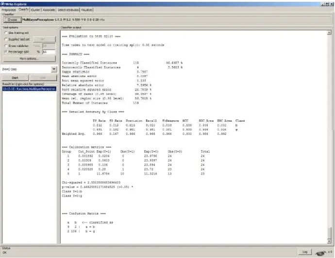
The calculation of Chi-square value and the corresponding p-value was introduced as a modification of the latest development version of Weka, which, at the time of the writing is 3.7.11. A sample execution with calibration metrics of the Weka Explorer module can be seen in Figure 1. In order to enable automated algorithm evaluation, these new metrics were also introduced in the Weka Experimenter module, which allows batch execution.
One of the weaknesses of the Hosmer-Lemeshow groups of risk approach is that, in poorly calibrated classifiers, it may not be possible to perform the division in the required number of groups, making further computations impossible. We have used the Percentile class implemented in the Apache Commons Mathematics Library, which follows the approach recommended by the US National Institute of Standards and Technology (5). It must be noted however, that there is no gold standard for the division in percentiles. Different software packages (such as SPSS, Stata, SAS, SciPy, Octave or R) implement diverse methods of estimation. Some of them let the operator choose one or another. Therefore, percentile group cut points may vary compared to the output generated by our modification of Weka, especially with small datasets and models with inadequate calibration.
Even if the number of groups is sufficient, the sum of estimated probabilities for a given group may be zero or close to zero. In order to slightly mitigate this problem, we set the number of groups at 5, as a lower number of groups was likely to produce more computable cases.
FIGURE 1. Hosmer-Lemeshow groups of risk Weka implementation
Classifiers and Datasets
SVMs with RBF and polynomic kernels, ANNs, C4.5 decision trees, KNNs, RIPPER, BayesNet and Naïve bayes classifiers were used on six canonical datasets (6-11). Dataset characteristics are presented in Table 1. We decided to include a mix of datasets with a variety of instances per independent variable.
One hundred experiments were performed with each algorithm and dataset using random-order train-test partitions of 66% (i.e. test datasets included 34% of the data). Classifiers were used as-is in all cases, with no parameter optimization. SVMs were adjusted to produce a logistic model with a probabilistic output.
TABLE 1. Datasets used in our experiments.
Dataset Train set size (66% of total instances)
Number of independent variables
German Credit data (6) 660 20
Final settlements in labor negotiations in Canadian industry database (7)
37 16
Ionosphere database (8) 231 34
Pima Indians diabetes database (9)
507 8
Breast cancer data (10) 188 9
United States Congressional Voting Records Database (11)
287 16
Comparison Methodology
Test set Chi-square values were compared between classifiers. Both high and incomputable values of this metric imply bad calibration, while adequate calibration is defined by a low Chi-square. Hence, the value was dichotomized at a cutoff point of 9.4877, which is approximately equivalent to a cumulative probability of 95% in a Chi-square distribution with 3 degrees of freedom. By this definition, RIPPER, C4.5 and KNN had less than 3 well-calibrated experiments each, which can be attributed to chance in the train-test partition rather than meaningful results. These classifiers were excluded from further comparisons. A GEE regression, using the dataset as a panel variable, was applied to the remaining algorithms in order to estimate their respective performance. The Naïve Bayes classifier was taken as a reference.
Average precision and average AUC were also added to the comparison in order to provide some context of the usual measures.
RESULTS
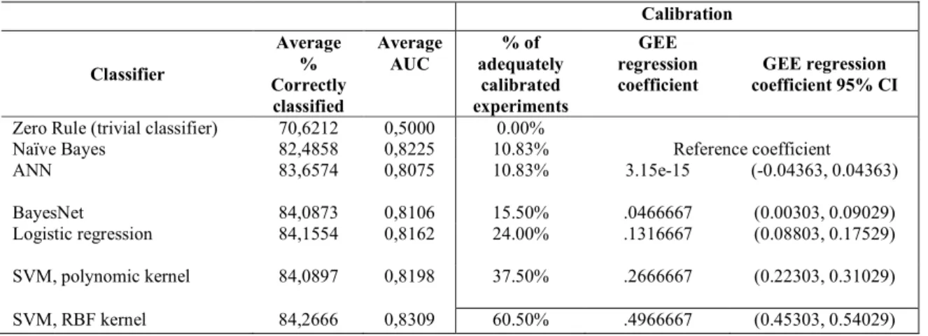
A comparison of classifier calibration performance against Naïve Bayes is presented in Table 2. There is no statistically significant difference between it and the ANN classifier in terms of calibration. SVMs with RBF (logistic) kernel exhibit the best results.
TABLE 2. Classifier performance
Calibration Classifier Average % Correctly classified Average AUC % of adequately calibrated experiments GEE regression coefficient GEE regression coefficient 95% CI
Zero Rule (trivial classifier) 70,6212 0,5000 0.00%
Naïve Bayes 82,4858 0,8225 10.83% Reference coefficient
ANN 83,6574 0,8075 10.83% 3.15e-15 (-0.04363, 0.04363)
BayesNet 84,0873 0,8106 15.50% .0466667 (0.00303, 0.09029)
Logistic regression 84,1554 0,8162 24.00% .1316667 (0.08803, 0.17529) SVM, polynomic kernel 84,0897 0,8198 37.50% .2666667 (0.22303, 0.31029) SVM, RBF kernel 84,2666 0,8309 60.50% .4966667 (0.45303, 0.54029)
In the case of ANN, most likely, better results could have been achieved with larger training datasets and parameter optimization.
This example shows that models with an acceptable AUC may not be adequately calibrated, which highlights its importance.
CONCLUSIONS
We have successfully developed a new functionality in the Weka data mining software and proved that it can be used as an additional metric of classifier performance.
In our tests well-calibrated models were rarely achieved with some classifiers. This is hardly surprising as some of the datasets were challenging and most classifiers used in machine-learning emphasize discrimination over calibration by design.
FUTURE WORK
For the sake of simplicity we have tested calibration measures in binary problems, which are common in many domains. Although the Hosmer-Lemeshow groups of risk approach may be generalized to multinomial problems, additional adjustments are usually required for adequate interpretation in these cases. Alternative approaches, some of them developed specifically for data mining problems may be preferable (12-14).
ACKNOWLEDGMENTS
The work leading to these results has received funding from the European Union under grant agreement n° 287678. It has also been supported by INAPRA (MICINN, DPI2010-21247-C02-02) project.
Authors also thank all the other members of the Speech Technology Group for the continuous and fruitful discussion on these topics.
REFERENCES
1. Cohen I, Goldszmidt M. Properties and benefits of calibrated classifiers. Knowledge Discovery in Databases: PKDD 2004: Springer; 2004. p. 125-36.
2. Hosmer Jr DW, Lemeshow S. Applied logistic regression: John Wiley & Sons; 2004.
3. Hall M, Frank E, Holmes G, Pfahringer B, Reutemann P, Witten IH. The WEKA data mining software: an update. ACM SIGKDD explorations newsletter. 2009;11(1):10-8.
4. Bartlett J. The Hosmer-Lemeshow goodness of fit test for logistic regression. 2014 [2014-06-09]; Available from: http://thestatsgeek.com/2014/02/16/the-hosmer-lemeshow-goodness-of-fit-test-for-logistic-regression/. 5. NIST. Percentiles. [2014-07-13]; Available from:
http://www.itl.nist.gov/div898/handbook/prc/section2/prc252.htm.
6. Hofmann H. German Credit data. Institut für Statistik und Ökonometrie Universität Hamburg2000. 7. Matwin S. Final settlements in labor negotitions in Canadian industry database. Computer Science Dept,
University of Ottawa1988.
8. Sigillito V. Ionosphere database. Applied Physics laboratory, The Johns Hopkins University1989.
9. Sigillito V. Pima indians diabetes database. Applied Physics laboratory, The Johns Hopkins University, laurel, MD1990.
10. Zwitter M, Soklic M. Breast cancer data. Institute of Oncology, University Medical Centre Ljubljana, Yugoslavia1988.
11. Schlimmer J. United States Congressional Voting Records Database. 1984
12. Bennett PN, editor. Using asymmetric distributions to improve text classifier probability estimates. Proceedings of the 26th annual international ACM SIGIR conference on Research and development in informaion retrieval; 2003: ACM.
13. Garczarek U. Classification Rules in Standardized Partition Spaces: Dissertation, Fachbereich Statistik, Universitat Dortmund, Dortmund, Germany. URL http://hdl. handle. net/2003/2789.(148); 2002.
14. Zadrozny B, Elkan C, editors. Transforming classifier scores into accurate multiclass probability estimates. Proceedings of the eighth ACM SIGKDD international conference on Knowledge discovery and data mining; 2002: ACM.