Active Learning for Data Streams
by
Saad Mohamad
A thesis submitted in partial fulfillment for the
degree of Doctor of Philosophy
in the
Department of Computing at Bournemouth University and
Department of Informatique et Automatique at IMT Lille Douai
With the exponential growth of data amount and sources, access to large collec-tions of data has become easier and cheaper. However, data is generally unlabelled and labels are often difficult, expensive, and time consuming to obtain. Two learn-ing paradigms have been used by machine learnlearn-ing community to diminish the need for labels in training data: semi-supervised learning (SSL) and active learn-ing (AL). AL is a reliable way to efficiently buildlearn-ing up trainlearn-ing sets with minimal supervision. By querying the class (label) of the most interesting samples based upon previously seen data and some selection criteria, AL can produce a nearly op-timal hypothesis, while requiring the minimum possible quantity of labelled data. SSL, on the other hand, takes the advantage of both labelled and unlabelled data to address the challenge of learning from a small number of labelled samples and large amount of unlabelled data. In this thesis, we borrow the concept of SSL by allowing AL algorithms to make use of redundant unlabelled data so that both labelled and unlabelled data are used in their querying criteria.
Another common tradition within the AL community is to assume that data sam-ples are already gathered in a pool and AL has the luxury to exhaustively search in that pool for the samples worth labelling. In this thesis, we go beyond that by applying AL to data streams. In a stream, data may grow infinitely making its storage prior to processing impractical. Due to its dynamic nature, the underlying distribution of the data stream may change over time resulting in the so-called
concept drift or possibly emergence and fading of classes, known as concept evolu-tion. Another challenge associated with AL, in general, is thesampling bias where the sampled training set does not reflect on the underlying data distribution. In presence ofconcept drift, sampling bias is more likely to occur as the training set needs to represent the underlying distribution of the evolving data. Given these challenges, the research questions that the thesis addresses are: can AL improve learning given that data comes in streams? Is it possible to harness AL to handle changes in streams (i.e., concept drift and concept evolution by querying selected samples)? How can sampling bias be attenuated, while maintaining AL advan-tages? Finally, applying AL for sequential data steams (like time series) requires new approaches especially in the presence of concept drift and concept evolution. Hence, the question is how to handle concept drift and concept evolution in se-quential data online and can AL be useful in such case?
In this thesis, we develop a set of stream-based AL algorithms to answer these ques-tions in line with the aforementioned challenges. The core idea of these algorithms is to query samples that give the largest reduction of an expected loss function that measures the learning performance. Two types of AL are proposed: decision theory based AL whose losses involve the prediction error and information theory
and parameter estimation can be derived from the proposed AL algorithms. Sev-eral experiments have been performed in order to evaluate the performance of the proposed algorithms. The obtained results show that our algorithms outperform other state-of-the-art algorithms.
This PhD thesis has been co-funded by Bournemouth University and IMT Lille
Douai (Ecole Mines-Tlcom, IMT-Universit de Lille) under the supervision of Prof. Hamid Bouchachia and Prof. Moamar Sayed-Mouchaweh. My time at Bournemouth and Douai has been influenced and guided by a number of people to whom I am
deeply indebted. Without their help, friendship and support, this thesis would likely never have seen the light of day.
I would like to thank the members of my thesis committee, Prof. Abdelhamid Bouchachia and Prof. Moamar Sayed-Mouchaweh for their insights and guidance. I feel most fortunate to have had the opportunity to receive their support. My
supervisors, Prof. Abdelhamid Bouchachia and Prof. Moamar Sayed-Mouchaweh, have had the greatest impact on my academic development during my thesis. They have been a tremendous mentor, collaborator and friends, providing me
with invaluable insights about research and academic skills in general. They both taught me how to do research, how to ask the right questions and how to answer them, how to have a clear vision and strategy. Their wisdom, creativity, integrity,
humility, and generosity will continue to inspire me. I was indeed fortunate to have them as my supervisors. I feel exceedingly privileged to have had their guidance and I owe them a great many heartfelt thanks.
My deepest gratitude and appreciation is reserved for my family. Without their
constant love, support and encouragement, I would never have been able to pro-duce this thesis. I dedicate this thesis to them.
Abstract ii Acknowledgements iv List of Figures ix List of Tables x Abbreviations xi Symbols xii 1 Introduction 1 1.1 Background . . . 1 1.2 Online Learning . . . 4 1.3 Active Learning . . . 6 1.3.1 Querying Criteria . . . 6
1.3.2 Online Active Learning . . . 8
1.3.3 Sampling Bias . . . 9
1.4 Aims and Objectives . . . 10
1.5 Contributions . . . 11
1.6 Structure of the Thesis . . . 12
1.7 List of Publications . . . 14
2 Active Learning for Data Streams under Concept Drift 16 2.1 Introduction . . . 17
2.2 Online bi-criteria AL . . . 19
2.2.1 Growing Gaussian Mixture Model (GGMM) . . . 23
2.2.2 Logistic regression . . . 25
2.2.2.1 Bayesian view of online logistic regression . . . 25
2.2.2.2 Handling of concept drift . . . 27
2.3 Online sampling . . . 28
2.3.1 Tackling the problem of sampling bias . . . 30 vi
2.5 Experiments . . . 33
2.5.1 Simulation on synthetic data . . . 34
2.5.1.1 Simulation on synthetic data . . . 35
2.5.2 Performance Analysis . . . 38
2.5.3 Simulation on real-world data . . . 40
2.5.4 Discussion . . . 41
2.6 Conclusion . . . 42
3 Active Learning for Data Streams under Concept Drift and Con-cept Evolution 43 3.1 Introduction . . . 44
3.2 Active Learning Approach . . . 46
3.3 Estimator Model . . . 51 3.3.1 Dirichlet process . . . 51 3.3.2 Proposed Model . . . 53 3.3.2.1 Clustering . . . 54 3.3.2.2 Semi-supervised classifier . . . 57 3.4 Experiments . . . 59 3.4.1 datasets . . . 61 3.4.2 Classification performance . . . 63 3.4.2.1 Settings . . . 63 3.4.2.2 Performance Analysis . . . 64
3.4.3 Class discovery performance . . . 66
3.4.3.1 Settings . . . 67
3.4.3.2 Performance Analysis . . . 68
3.5 Conclusion . . . 70
4 Active Learning for Sequential Data Streams: An Application to Human Activity Recognition 71 4.1 Introduction . . . 72
4.2 Related Work and Motivation . . . 75
4.3 Conditional Restricted Boltzmann Machine. . . 77
4.4 Online Semi-supervised Classifier . . . 79
4.4.1 Prediction:. . . 80
4.4.2 Updating: . . . 82
4.4.3 Re-sampling: . . . 84
4.5 Active Learning Approach . . . 85
4.6 Experiments . . . 90
4.6.1 Feature extractor . . . 91
4.6.2 Classification performance . . . 93
4.6.2.1 Locomotion . . . 94
4.6.2.2 Gestures . . . 96
4.7 Conclusion . . . 101
5 Conclusions and Future Work 104
5.1 Conclusion . . . 104
5.2 Future Work . . . 106
A 109
A.1 Parameters setting of Growing Gaussian Mixture Model. . . 109
B 112
B.1 Compute Eq. (3.22): . . . 112
B.2 Compute the first term of Eq. (3.31): . . . 113
C 114
C.1 Computation of Eq. (4.28) . . . 114
C.2 Sampling precision hyper-parameters . . . 117
2.1 General scheme of BAL. . . 20
2.2 Combining clustering and classification for AL . . . 21
2.3 The main steps of GGMM . . . 24
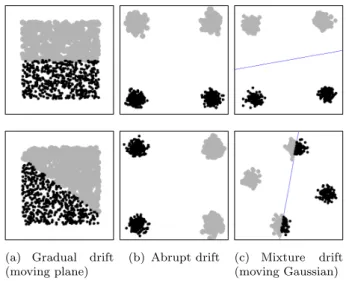
2.4 Synthetic data. . . 34
2.5 UAL gradual drift. . . 36
2.6 BAL gradual drift . . . 36
2.7 UAL abrupt drift . . . 36
2.8 BAL abrupt drift . . . 37
2.9 UAL mixture drift . . . 37
2.10 BAL mixture drift . . . 37
2.11 Effect of the number of clusters on the performance . . . 39
2.12 Sensitivity to remote drift . . . 39
2.13 Results related to the real-world datasets . . . 42
3.1 General scheme of SAL . . . 50
3.2 Graphical model . . . 52
3.3 Infinite mixture model . . . 53
3.4 Proposed semi-supervised clustering model . . . 57
3.5 Classification performance . . . 65
3.6 Active learning behaviour along the stream for Electricity. . . 65
3.7 Comparison of the class discovery performance . . . 69
4.1 General Architecture of CRBM-OSC-BSAL . . . 75
4.2 Feature Extractor Architecture (r1 = 2, r2 = 1) . . . 78
4.3 Graphical model of OSC . . . 79
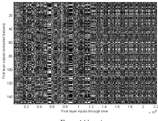
4.4 Layer 1. . . 92
4.5 Layer 2. . . 93
4.6 Layer 3. . . 94
4.7 Labelling rate along the stream of subject 2 (S2). . . 100
4.8 Labelling rate along the stream of subject 3 (S3). . . 100
4.9 Labelling rate along the stream of subject 4 (S4). . . 101
A.1 Gradual drift . . . 111
A.2 Mixture drift . . . 111
A.3 Electricity . . . 111
A.4 Airlines . . . 111 ix
1.1 Comparisons. . . 13
2.1 Clustering parameters (empirically obtained) . . . 40
2.2 Effect of the number of clusters on BAL accuracy: case of plane and Gaussian data . . . 40
2.3 Accuracy of BAL compared with random sampling using different budget values (Synthetic data) . . . 40
2.4 Characteristics of the real-world datasets . . . 40
3.1 Benchmark Datasets properties used for comparing SAL against [1] 62 3.2 Benchmark Datasets properties used for comparing SAL against [2, 3] . . . 62
3.3 Learning rate parameters . . . 64
3.4 SAL hyper-parameters setting . . . 64
3.5 Number of classes discovered by different methods . . . 68
3.6 Average class accuracy achieved using different methods . . . 68
4.1 Real AR Dataset propreties used for evaluating CRBM-OSC-BSAL 91 4.2 Class proportions for gesture activities . . . 91
4.3 Class proportions for locomotion activities . . . 91
4.4 Real AR Dataset propreties used for evaluating CRBM-OSC-BSAL 91 4.5 Classification performance for locomotion activities undersetting 1 95 4.6 Classification performance for locomotion activities undersetting 2 95 4.7 Classification performance for locomotion activities . . . 96
4.8 Classification performance for gesture activities under setting 1 . . 97
4.9 Classification performance for gesture activities under setting 2 . . 98
4.10 Classification performance for locomotion activities (5%) . . . 99
4.11 Classification performance for gesture activities (5%) . . . 102
4.12 Classification performance for gesture activities (10%) . . . 103
AL Active Learning
MQS Membership query Synthesis PPP Poole-based SelectiveSampling SSS Stream-basedSelectiveSampling QBC Query-By-Committee
HAR Human Activity Recognition BAL Bi-criteria Active Learning
GGMM Growing GaussianMixture Model MAP Maximum-A-Posteriori
MLE Maximum Likelihood Estimation GMM Gaussian Mixture Model
EM Expectation Maximisation UAL Uni-criterion Active Learning SAL Stream-basedActive Learning DP Dirichlet Process
DPMM Dirichlet ProcessMixture Model NIW Normal-Inverse-Wishart
AA AverageAccuracy ACA AverageClassAccuracy
CRBM Conditional Restricted Boltzmann Machine OSC Online Semi-supervised Classifier
BSAL Bayesian Stream-based Active Learning
DL Deep Learning
DT Decision Tree
SVM Support Vector Machine
Symbol Description
X set of data samples
XU set of unlabelled data
XL set of labelled data
YL set of labels associated with XL
Xt set of data samples seen up to time t
XLt set of labelled data samples seen up to time t
XUt set of unlabelled data samples seen up to time t
Y set of data labels
YLt set of labels associated with XLt
D =(X, Y)
DL =(XL, YL)
Dt = (Xt, YLt)
DLt = (XLt, YLt)
Ct the set of classes discovered up until time t
yt true data label at time t
ˆ
yt predicted data label at time t
xt data input at time t
R risk
ˆ
R expected Risk
R(θ) risk given θ (classifier parameter) ˆ
Rn(θ) empirical risk over n samples
ˆ
RXU(θ) empirical risk over unlabelled data XU
L(.) loss function
Introduction
In this chapter, we present a general background on machine learning, its im-portance and paradigms; in particular online learning and active learning. We introduce the challenges of online learning from data streams. We also discuss the relevance of active learning as well as the main approaches, with particular focus on stream-based active learning. A literature review on this later is presented, where the state-of-art competitors of our new algorithms proposed in this the-sis are described. Finally, the research questions, contributions and structure of the thesis are presented.
The organization of this chapter is as follows. Section 1.1 is a background. Sec-tion 1.2 introduces online learning and its challenges. Section 1.3 reviews active learning with focus on the state-of-the-art stream-based active learning algorithms. Section1.4presents the aim and objectives of the thesis. Section 1.5 discusses the contributions of the thesis. The structure of the thesis is presented in Sec. 1.6. A list of the publications on which the thesis is based is shown in Sec. 1.7.
1.1
Background
Our digital universe is rapidly growing. According to an updated digital universe study [4], in 2020, the amount of digital data produced will exceed 40 zettabytes which is the equivalent of 5,200 GB of data for every man, woman and child on earth. The abundance of data has been exploited and generated a major impact in many fields of application like manufacturing, health-care, media, sports, science
and more. In order to exploit such data, for the sake of decision making, machine learning (ML) techniques can be used.
ML has a long history in applied mathematics and statistics. ML community has been exceedingly creative at taking existing ideas across many fields and mixing and matching them to solve problems in different domains [5]. From statistical inference point of view, ML can be categorised into two views: Frequentist view
andBayesian view. Bayesian inference is performed with probabilistic parameters (model’s parameters) and fixed data, while Frequentist inference is performed with fixed parameters and random data samples. In the Frequentist approach, unknown set of parameters is treated as having fixed unknown values. It cannot be envisioned as random variables. In contrast, the Bayesian approach does allow probabilities to be associated with the unknown parameters. In ML literature, we can distinguish the following paradigms.
• Supervised learning (SL).
• Unsupervised learning (UL).
• Semi-supervised learning (SSL).
• Reinforcement learning (RL).
• Active learning (AL).
SL is about learning a mapping function, f : X → Y, between a set of input instances and their corresponding output (e.g., labels of classes). The training set
D = (X, Y) is used to find the mapping (model) with the least expected loss. If the output is categorical, SL is a classification task; otherwise it is a regression task. Classification is a supervised learning task where the labels that we wish to predict take discrete values.
In UL, we are not given any output to use for training D = {x1, ...,xN}. UL
encompasses clustering where we try to find groups of data instances that are similar to each other. Loss function here is sometimes called objective function
(e.g., K-Means algorithm).
SSL, as its name implies, falls between UL and SL. It can be thought of as a class of supervised learning that also makes use of unlabelled data for training. SSL makes use of one of the following assumptions.
• Smoothness assumption: points which are close to each other are more likely to share the same class label.
• Cluster assumption: the data tends to form discrete clusters and points in the same cluster are more likely to share a label (this is special case of the smoothness assumption)
• Manifold assumption: the data lies approximately on a manifold of much lower dimension than the input space.
In RL, the output is a reward given by the environment according to its state as a result of certain provided input (action) by the learner (agent). Thus, given a state s and an action a, the environment feedback is a reward function R(s, a). Unlike SL, where we receive inputs and outputs from the environment and tries to learn a model, RL agent interacts with the environment and try to learn a policy
f that maximizes cumulative rewards, where f :A×S →R and A, S, R are the set of actions states and rewards respectively.
AL is about interacting with an oracle to query the label of selected data instances. In contrast to RL, the actions space is just queries and the reward is the true label. Once obtained, the data instances and their labels are used to train SL algorithms. We should point out that AL can be used to ask questions of different form than querying certain data [6,7]. However in this research work, we consider AL that queries data labels for classification purposes. On the other hand, passive learning is a terminology that will be used for any learner that receives passively the information provided (class label in our case).
ML algorithms can also be classified according to the way data is processed. We can distinguish two paradigms: online learning and offline learning. In offline learning, once the training phase is exhausted, the model is no more capable to learn further knowledge from new instances, that is, it is not able to self-update in the future. On the contrary, in online setting, data comes in a form of streams and the model must predict and adapt online, that is, it keeps learning over time. For example, a spam detector receives online message and the task is to predict whether the messages are spam or not. The quality of the model’s prediction is assessed by a loss function that measures the discrepancy between the predicted label and the true one. Then, an adaptation of the model is applied if needed.
Since this thesis is about online active learning, in the following, we provide more details related to online learning and active learning.
1.2
Online Learning
Online learning has been studied in several research fields including game theory, information theory, data mining and machine learning [8–13]. The concept of
online learning may be interpreted differently. Any online learning algorithm must be able to learn from data streams. The characteristics of data stream include [14]:
• Continuous flow (data samples arrive one after another.
• Huge data volumes (possibly of an infinite length).
• Rapid arrival rate (relatively high with respect to the processing power of the system).
• Susceptibility to change (data distributions generating examples may change over time).
Therefore, an online learning algorithm should fulfil the following requirements:
• The algorithm can access data only once and sequentially,
• The time and space complexity of the algorithm must not scale with the number of instances,
• The algorithm should be able to self-adapt.
Incremental learning [15–18] is sometime mistaken for online learning, but it can-not fulfil all the listed requirements. Although, it processes one instance or a mini-batch of instances at each iteration, it requires to cycle over the whole data many times. Besides, incremental learning algorithms cannot adapt to changes. Online learning presented in [8, 9, 19], views data samples as the product of some unknown and unspecified mechanism that could be deterministic, stochastic, or even adversarial adaptive to the algorithm behaviour. In this thesis, we focus on online learning from data streams with non-adversarial actions. Many such algo-rithms can be derived from their offline counterparts. To do so, algoalgo-rithms require
adjustment to make online update and mechanisms to forget outdated data and adapt to changes [20].
Some algorithms can be naturally updated online (e.g., k-nearest neighbours and naive-Bayes) and only require mechanisms to deal with changes [20–22]. Others, like decision trees, require, in addition to mechanisms for dealing with changes, substantial adjustments to make online update [23, 24]. Details on mechanisms and techniques for online learning methods can be found in [20, 25].
In this thesis, we adopt sequential Bayesian approaches for learning from non-stationary data streams [26–29]. That is, the sequential nature of Bayes theorem is exploited to recursively update some models. Forgetting factors [30] are employed to decay the contributions from old data points in favour of new better ones. As mentioned earlier, data streams are susceptible to changes over time resulting in the so-called concept drift or the possible emergence of classes, known as con-cept evolution. Concept drift occurs when the statistical properties of the target variable, which the model is trying to predict, change over time in unforeseen ways [21]. More precisely, we can distinguish two types of drifts:
• Real concept drift refers to changes in the conditional distribution of the targets (labels) p(y|x) given the observations. Such changes can happen either with or without change in the marginal distribution of the incoming data p(x).
• Virtual drift occurs if the distribution of the incoming data changes p(x) without affecting p(y|x). Hence, in both cases the joint distribution p(x, y) changes.
Concept evolution occurs when new classes emerge [31–33]. Emergence of new classes has been studied in the context of novelty detection where classification models are unable to detect the novel class until they are trained with labelled instances of it. In this thesis, concept evolution is defined as emergence of new unseen classes as the data streams evolve over time.
Finally, we give an illustrative example of a simple online learning algorithm called perceptron. The perceptron [34–36] is perhaps the first and simplest online learn-ing algorithm. Perceptron uses a class of linear separators in the input space,
where the prediction of the data label depends on the side of hyperplane the data instance falls in. If the predicted label and the true label are different, the algorithm adjusts itself.
h(x) = 1 w. 1x >0 −1 otherwise A simple perceptron consists of the following steps:
1. Initialise the weights w. 2. Receive the input xt.
3. Predict the output by computing ˆy=h(xt).
4. Update w if yt 6=h(xt): wt+1 =wt+αytxt, where α is a learning rate and
yt is the true output.
1.3
Active Learning
In the context of classification, AL allows to label some selected data samples by an expert (oracle or annotator) according to some selection criteria. The overall goal of AL is to provide, at least, the same performance as that of passive learning while using less labelled examples.
1.3.1
Querying Criteria
There exist three main approaches of AL [37]: membership query synthesis (MQS), pool-based selective sampling (PSS) and stream-based selective sampling (SSS). According to MQS, the learner generates new data samples from the feature space that will be queried. However, labelling such arbitrary instances may be im-practical, especially if the oracle is a human annotator as we may end up querying instances [38] that are hard to explain. PSS is the most popular AL method, ac-cording to which the selection of instances is made by exhaustively searching in a large collection of unlabelled data gathered at once in a pool. Here, PSS evaluates and ranks the entire collection before selecting the best query. On the other hand,
SSS scans through the data sequentially and makes query decisions individually. In the case of data streams, PSS is not appropriate, especially when memory or processing power is limited. It also assumes that the pool of data is stationary and uses the whole dataset. This will delay the adaptation and waste the resources. SSS, instead, adapts the classifier in real-time leading to fast adaptation.
While there have been many AL studies on the offline variant, only few ones have investigated the online setting. Most of the AL sampling criteria have been first introduced for offline setting, then adapted to work online. Authors in [39] introduce one of the most general frameworks for measuring informativeness, label uncertainty sampling criterion, where the queried instances are those which the model is most uncertain about their label. It has been since then used in many successful offline AL algorithms [40–44].
Another popular AL sampling criterion framework is thequery-by-committee [45]. Here, a committee of models trained on the same dataset are maintained. They represent different hypotheses. The data label about which they most disagree is queried. To use thequery-by-committee framework, one must construct a commit-tee of models and have some measure of disagreement. Query-by-committee has shown both theoretical and empirical efficiency in several offline AL studies[46–48].
Density-based is another AL sampling criterion that differs from uncertainty and
query-by-committeein that it uses unlabelled data for measuring the instance infor-mativeness [44]. Density-based criterion assumes that the data instances in dense regions are more important. Many studies have involved density-based criterion by combining it with other criteria like uncertainty sampling [49] and Query-by-committee sampling [50].
Authors in [51] point out that there is no individual AL method superior to the others and that their combination could produce better results. A reasonable ap-proach to combine an ensemble of active learning algorithms might be to evaluate their individual performance and dynamically switch to the best performer so far [51]. This idea of rewarding is rooted in RL [52]. There exists a classical trade-off in RL called the exploration/exploitation trade-off which can be explained as fol-lows. If we have already found a way to act in the domain that gives a reasonable reward, then is it better to continue exploiting the explored domain or should we try to explore a new domain in the hope that it may improve the reward [53]. This concept dates back to the study of bandit problems in 1930s which are the most basic examples of sequential decision problems with an exploration-exploitation
trade-off. Because of the strong theoretical foundation of bandit problems, they are exploited by many authors to formulate AL [51, 54, 55]. However, none of them considers SSS active learning.
1.3.2
Online Active Learning
Online AL methods for data streams in presence of drift have been dealt with using batch-based learning, where data is divided into batches [56, 57]. These methods assume that the data is stationary within each batch and then PSS AL strategies are applied. Authors in [58] use a sliding window approach, where the oldest instances are discarded. Label uncertainty is, then, used to label the most informative instances within each new batch. In [59] an online approach is com-pared against a batch based approach, finding that both have similar accuracy, but the batch-based one requires more resources. Moreover, the batch-based approach requires to specify the size of the batch. Some studies consider fixed size; others use variable one. However, in both cases, more memory than the one with the on-line approach is needed. Another issue is that, in general, batch-based approaches cannot learn from the most recent examples until a new batch is full. This leads to more delay when responding to changes. This delay has a negative effect leading to late recovery. All these reasons make online learning more natural and suitable for AL.
Few SSS AL studies have been proposed [1, 3, 60–62]. Methods in [60, 61] as-sume that the data is stationary. They cannot work in the case of evolving data streams as the models cannot perceive the change of data distribution. Thus, these methods lead tosampling bias [63] problems when data evolves (see Sec. 1.3.3). Authors in [3], handle the problem ofconcept evolutionby defining a non-parametric Bayesian prior on the classes using Pitman-Yor Processes [64]. However, they use
Query-by-committee (QBC) [45] which aims at reducing the version-space instead of directly optimizing the error rate. QBC often fails by spending effort eliminat-ing areas of parameter space that have no effect on the error. It does not consider the data distribution effect and ignores the problem of sampling bias. It is worth noting that although this method is stream-based AL, it memorizes all labelled samples and re-use them at each iteration for updating the model.
Online AL approaches that address the three data stream challenges: infinite length,concept drift andconcept evolution are the rarest. Authors in [65] also deal with concept evolution and concept drift. They apply a hybrid batch-incremental learning approach, where the data is divided into fixed-size chunks and an offline classifier is trained from each chunk. An ensemble of M classifiers is maintained to classify the unlabelled data. To detect the novel classes, a clustering technique is used in order to isolate odd data instances. If the isolated samples are enough and sufficiently close to each other (coherent), they get queried. Otherwise, the algorithm considers them as noise. The algorithm also uses the uncertainty sam-pling within the current chunk to query the label of instances for which it is most uncertain. This algorithm does not address sampling bias and it needs to store the data instances in different batches.
1.3.3
Sampling Bias
Sampling bias problem is, in general, associated with AL, where the sampled
training set does not reflect on the underlying data distribution. Basically, AL seeks to query samples that, if labelled, significantly improve the learning. AL becomes increasingly confident about its sampling assessment. That confidence could lead, however, to negligence of valuable samples that reflect on the true data distribution. It, therefore, creates a bias towards a certain set of instances, which could become harmful. Sampling bias problem is more severe in online setting as the underlying classifier used by AL has to adapt. On the other hand, the adaptation can depend on the queried data. Hence, if drift occurs for samples which the model is confident about their labels, they will not be queried and the model will not be adapted.
Methods in [1,62] takessampling biasproblem into account. In [1], SSS is adopted using randomization to avoid bias estimation of the class conditional distribution that may result from querying. This randomization is combined with label un-certainty to deal with concept drift. However, it results in wasting resources by randomly picking data to cover the whole input space. Moreover, randomization has no interaction when drift occurs and it naively keeps querying randomly. In [62], sampling bias is studied using importance weighting principle to re-weight labelled data and remove the bias. Importance weighting principle has been the-oretically proven to be effective [66]. However, the method in [62] is restricted
to binary classification. Both methods [1, 62] assume that the number of classes is fixed and known in advance, namely there is no concept evolution. Further-more, they ignore the effect of data distribution and do not benefit of abundant unlabelled data samples.
1.4
Aims and Objectives
Using AL in real world scenarios is not an easy task as many constraints and side effects arise. Most of the studies have been associated with unrealistic assumptions such as:
1 The data can be re-accessed at any time.
2 The number of classes is a-priori known (no concept evolution). 3 The data is stationary (no concept drift).
4 The data stream samples are temporally independent from each others.
The main aim of this thesis is to make AL applicable in realistic real-world sce-narios. Since data comes as a stream, online learning classifiers and SSS active learning algorithms should be adopted. AL for data streams with concept drift
could suffer the problem ofsampling bias. For example, in classification, label un-certainty aims at selecting the most uncertain instances that typically lie close to the classification boundary. Training the classifier on those instances is expected to adjust the boundary and achieving better classification accuracy. However, given the non-stationary aspect of data coming over time in a stream,concept drift may occur any time and anywhere in the feature space. Applyinglabel uncertainty may result in missing the changes occurring farther from the boundary. Here, the sam-pled instances are biased towards the boundary rather than being representative of the underlying data distribution. The evolving nature of data streams leads to
concept evolution which poses another challenge for using AL to learn from data streams. That is, AL algorithms should not only query informative samples, but also discover the class space. This task becomes even more challenging in the case of data involving classes of unbalanced proportions. Applying AL for sequen-tial data steams with temporal dependency requires new approaches especially in
presence of concept drift and concept evolution. That is, how to take the tempo-ral dependency of the data into consideration when querying. To the best of our knowledge, this work is original considering the training data as a set of sequences (with temporal dependency within sequences); while existing AL work has focused on data assumed being drawn independently and identically (iid) from some joint distribution P.
In a nutshell, the objectives of this thesis:
• To provide a uniform probabilistic approach to cope with active learning taken into account inherent phenomena.
• To investigate active learning in the context of Streaming using various querying criteria.
• To investigate decision-theory based and information-theory based active learning in the context of stream-based selective sampling.
• To develop innovative application for AL from sequential data streams.
Section1.5 provides a more precise description of contributions in line with these objectives.
1.5
Contributions
Most AL approaches, including those mentioned in Sec. 1.3, are basically derived from the general approach of finding queries that yield the largest reduction of the expected loss. Let Ω denote the set of variables that can be fully random or include some random elements. LetLrefer to the loss function. The expected loss function that AL aims to reduce can be expressed as follows:
R=EΩ[L( ˆΩ,Ω)] (1.1)
where the hat refers to an estimated term. Depending on the loss functions in-volved, AL can be divided to two main groups: information-based and decision-based AL. These groups mainly differ in the type of loss functions used. While
AL losses involve the model parameter. The set of variables in Ω includes labelled and unlabelled data.
The contributions of the thesis can be summarised as follows:
1. We proposedecision theory andinformation theory AL algorithms that seek to directly reduce the expected loss online while taking the data streams challenges (infinite length,concept drift andconcept evolution) into account. 2. The proposed algorithms can handle concept drift and concept evolution by querying the data samples representative of them. Hence, they are changes aware.
3. Some of the proposed AL algorithms handle sampling bias problem.
4. The proposed AL algorithms uses both labels and unlabelled data.
In this thesis, we propose AL algorithms that query the samples which incur the highest reduction in the expected loss (Eq. (1.1)), while using both labelled (like in
uncertainty criteria) and unlabelled data (like in thedensity-based criterion). The proposed algorithms called BAL, SAL and BSAL (see abbreviations list for full names) address the challenges of AL for data streams (i.e., concept drift, concept evolution,sampling bias and temporal dependency). They handleconcept drift and
concept evolution by querying the data samples representative of them (i.e., their characteristics). In contrast to standard techniques for handlingconcept drift and
concept evolution [22,32,33,67, 68], where only automatic detection mechanisms are applied, AL assumes that an oracle provides the true labels of data. BAL and SAL aredecision theorybased AL approaches while BSAL is aninformation theory
based AL approach. The information based approach seems better at coping with
concept evolution when classes are unbalanced (See Chap. 4). Table 1.1 sums up the contributions of the thesis showing how such contributions compare against the closest state-of-the-art algorithms based on well-defined characteristics.
1.6
Structure of the Thesis
Table. 1.1Comparisons
AL uses Type of Data Type of AL Data Streams Challenges Sampling Bias Labelled data Unlabelled data Sequential Non-sequential Information-based Decision-based Concept drift Concept evolution
BAL X X X X X X SAL X X X X X X X BSAL X X X X X X [1] X X X X [3] X X X X [60] X X X X [61] X X X [62] X X X X X
• Chapter2shows how AL can be applied for classifying drifting data streams. A new online AL algorithm called BAL is proposed. BAL queries data sam-ples contributing to the reduction of the expected future error Eq. (1.1). Because the calculation of the expected future error is intractable, it is ap-proximated using online classification and online clustering models. Impor-tance weighting principle is used to curb the sampling bias problem, so that drifting samples are queried. The proposed approach only considers binary classification and does not deal with concept evolution.
• Chapter 3 proposes a new online AL algorithm, called SAL. It is capable of coping with bothconcept drift andconcept evolution. SAL seeks to minimize the expected future error. However, here the approximation is done using different estimation models (i.e., non-parameter Bayesian models). These models allow to cope with the lack of prior knowledge about the data stream, like the number of classes and data distribution. The minimization process is done, while tackling the problem of sampling bias so that samples that induce the change (i.e., drifting samples or samples coming from new classes) are queried.
• Chapter 4 proposes a new online information-based AL algorithm (BSAL)
that is able to cope with both concept drift and concept evolution. In con-trast to decision-based AL approaches, adopted by BAL and SAL whose losses involve the prediction error, information-based AL losses involve the model parameter. Hence, BSAL can elegantly handleconcept evolution since there is no need to heuristically modify the loss function to account for the new classes. More importantly, it can efficiently handle concept evolution
from data involving classes of unbalanced proportions. Another contribu-tion in this chapter is applying AL for sequential data streams with tempo-ral dependency. To cope with this challenge, we propose an algorithm with a three-module architecture composed of a feature extractor (CRBM) and an online semi-supervised classifier (OSC) equipped with the AL algorithm
BSAL. Knowing that the proposed approach is generic and not dedicated to specific application, human activity recognition (HAR) is used as a real-world application.
• Chapter 5 summarizes the key contributions of this thesis and provides a broad view of the future work. Particularly, how to address the delayed and noisy labelling challenges.
1.7
List of Publications
A number of publications have emerged from this research work with some of them still under review.
• Chapter 2 is based on the following publication:
– S. Mohamad, A. Bouchachia; M. Sayed-Mouchaweh, A Bi-Criteria Ac-tive Learning Algorithm for Dynamic Data Streams, IEEE Transactions on Neural Networks and Learning Systems, 2016.
Impact Factor: 6.108
• Chapter 3 is based on the following publications:
– S. Mohamad, M. Sayed-Mouchaweh, A. Bouchachia. Active Learning for Classifying Data Streams with Unknown Number of Classes. Neural Networks, accepted with minor revision, 2017.
Impact Factor: 5.287
– S. Mohamad, Moamar Sayed-Mouchaweh, and Abdelhamid Bouchachia. Active Learning for Data Streams under Concept Drift and concept evo-lution. Workshop STREAMEVOLV organised at the European Con-ference on Machine Learning, 2016.
• Chapter 4 is based on the following publications:
– S. Mohamad, M. Sayed-Mouchaweh, A. Bouchachia, Online Active Learning for Human Activity Recognition from Sensory Data Streams, Pattern Recognition, under review, 2017.
– S. Mohamad, A. Bouchachia, M. Sayed-Mouchaweh. A Non-parametric Hierarchical Clustering Model. The IEEE International Conference on Evolving and Adaptive Intelligent Systems (EAIS), pp:1-6, IEEE Press, 2015.
Active Learning for Data Streams
under Concept Drift
In this chapter, we address the challenges of applying AL for data streams which are concept drift and sampling bias. We propose a novel bi-criteria AL approach (BAL) that relies on label uncertainty criterion anddensity-based criterion. While the first criterion selects instances that are the most uncertain in terms of class membership, the latter dynamically curbs the sampling bias and avoids querying outlier by weighting the samples to reflect on the true underlying distribution. In order to design and implement these two criteria for learning from the data stream, BAL adopts a Bayesian online learning approach and combines online classification and online clustering through the use of online logistic regression
and online growing Gaussian mixture models respectively.
The organization of this chapter is as follows. Section2.1 is an introduction. Sec-tion 2.2describes the proposed selection criteria along with the used classification and clustering algorithms. Section2.3 provides the details of the proposed online sampling. Section 2.4 presents the algorithm. Section 2.5 discusses the experi-mental results for a number of well-known academic and real world datasets and Sec. 2.6 concludes the chapter.
2.1
Introduction
Classification has been the focus on large body of research due to its key relevance to numerous real-world applications. A classifier is trained by learning a mapping function between input and pre-defined classes. In an offline setting, the training of a classifier assumes that the training data is representative and is available prior to the training phase. Once this latter is exhausted, the classifier is deployed and, therefore, cannot be trained any further even if performs poorly. This can happen if the training data used does not exhibit the true characteristics of the underlying distribution. Moreover, for many applications data arrives over time as a stream and therefore the offline assumptions cannot hold. That is, the characteristics of data streams make it impractical to use offline learning algorithms: i) data streams are unbounded in size, ii) they arrive at high steady rate and iii) they may evolve over time. Thus, to deal with data streams efficiently, the classifier must(self-)adapt online over time [69,70]. To do that, the classifier needs to be fed with labeled data continuously which is not feasible in most real-world streaming situations where the data is usually unlabeled. It is therefore very important to seek well-informed ways to obtain labels. AL methods provide a systematic approach to select data examples whose labels should be queried. It reduces the cost of obtaining labelled data by querying much less examples to reach the same performance as when data samples are randomly queried.
For the sake of illustration, consider the example of internet advert popping up on screen where both online and active learning are relevant. The goal is to predict if an advert item will be interesting to a given shopper at a given time. To this end, a classifier is built based on the feedback from the shoppers. However, the interest and preference of the shoppers may change over time leading to what is known asconcept drift. Therefore, building a static model for such a scenario will not be effective; hence, the importance of an online adaptive model is manifested. In the streaming setting, obtaining unlabelled data is often cheap but labelling it is expensive. For instance, in the previous example, asking frequently for feedback whether an advert is interesting would annoy the shoppers; hence AL should be deployed in applications with caution.
Label uncertainty (or uncertainty sampling) is a simple and popular criterion and more important it is very suitable for online AL. However, selecting the data examples from the stream using label uncertainty leads to sampling bias as we
explained in Chap.1. On the other hand, density-based allows covering the whole input space with only few data samples [71] and reducing the sampling bias. In this work, we introduce a bi-criteria AL algorithm (BAL) for evolving data streams. Specifically, we combine label uncertainty and density-based labelling in an SSS-like setting. The uncertainty of data samples is evaluated using a classi-fication model while density of regions is evaluated using a clustering model. In general, density criterion performs efficiently with few labelled data since it sam-ples from maximum-density unlabelled regions. On the other hand, uncertainty criterion tunes the decision boundary after selective sampling from the uncertain regions [39, 72–74]. Thus, the density criterion is useful when there is regularity in the data which is the case of many applications. However, the density criterion alone would not provide an accurate classifier. In other words, the density crite-rion helps establishing the initial decision boundary; while uncertainty sampling ”fine-tunes” that boundary by sampling the regions where the classifier is least certain. By combining both criteria, we can take advantage of the density crite-rion to reduce the data examples required by the uncertainty critecrite-rion to build an accurate classifier.
To ensure enough flexibility of BAL, we explicitly distinguish between the learning engine and the selection engine. The learning engine uses a supervised learning algorithm to train a classifier on the existing labeled data, while the selection engine selects influential samples from the data stream for labelling. Here, the selection engine includes a classifier which is different from the classifier used by the learning engine and the clustering model that serves to design and deploy the two criteria.
AL stands as a very interesting opportunity to handle concept drift by querying the data samples representative of this drift (i.e., its characteristics). In contrast to standard concept drift handling techniques, where only automatic detection mechanisms are applied, in AL an access to the oracle that provides the ground truth (true labels of data) is granted. To this end, we use importance weighting
principle to weight labelled data samples that drives a drift in order to increase the importance of their regions in the feature space. Importance weighting prin-ciple has also been theoretically proved to correct sampling bias [75]. The BAL algorithm proposed in this work is the first AL algorithm that is concept drift
To illustrate how BAL behaves, consider the example that pertains to internet advertisement. Using uncertainty criterion only would result in querying adverts for which the classifier is uncertain and therefore by interactively labelling such adverts, the classifier can improve its performance towards a better prediction of what to propose to the shopper. On the other hand, the density criterion takes the similarity of the adverts into account. Thus, from a dense group of similar adverts only one which represents the whole group will be queried. Clearly combining the two criteria allows querying representative adverts for which the algorithm is not sure. Furthermore, in the streaming case, the interest and preference of the shoppers may change over time; hence when the change (drift) occurs in relation to those adverts for which the classifier is certain, thesampling bias caused by the active learning will be harmful. By implementing the weighting mechanism, we aim at reducing the sampling bias by labelling more of data samples that drive the drift and that make the uncertainty criterion less important for these data.
In a nutshell, the contributions in this chapter are:
1. We propose a novel online AL algorithm for data streams based on a proba-bilistic model that combines two querying criteria: uncertainty and density-based criteria. To the best of our knowledge this is the first approach based on density-uncertainty to the online setting.
2. The proposed combination brings classification through logistic regression and clustering through growing Gaussian mixture models together to imple-ment the two querying criteria in a uniform probabilistic way. The choice of these algorithms is therefore well motivated.
3. We propose mechanisms for making the proposed BAL algorithm aware of
concept drift. It is the first study that shows the effectiveness of AL in dealing with concept drift.
2.2
Online bi-criteria AL
The steps of the bi-criteria active learning algorithm (BAL) proposed in this work are portrayed in Fig. 2.1 and the corresponding details are discussed in Sec. 2.4. In a nutshell, BAL consists of 4 steps. In the first step, given an instance x, the
Figure. 2.1 General scheme of BAL
clustering model which is used to implement the density-based criterion is updated (see Sec. 2.2.1). Using BAL’s sampling model in the second step, the probability of querying is computed and the decision whether to query and carry on to the third step or discard the instance and receive new one is made (see Sec. 2.3). In the third step, the label corresponding to the queried instance x is received and the classification model which is used to implement the label uncertainty criterion will be updated (see Section 2.2.2). In the fourth step, a weighting technique is used to curb the sampling bias (see Section 2.3.1).
In order to identify the data examples to query, we seek to minimize the current expected error which consequently leads to the minimization of the future expected error. It can be seen that this error can be derived from Eq. (1.1) (see Chap.1) by using a prediction error loss function. The current expected error for an instance x can be computed using density-based and label uncertainty criteria which are estimated by dynamic classification and clustering models.
In [76] it is suggested to select samples that minimize the expected future classi-fication error given as follows:
Figure. 2.2 Combining clustering and classification for AL
R=
Z
x
E[(ˆy−y)2|x]p(x)dx (2.1) where y is the true label of data instance x and ˆy is the predicted output. E[.|x] denotes the expectation over p(y|x). This integral cannot be computed due to its complexity. Authors in [49], who proposed an AL method that relies on an offline pool-based selective sampling setting, noted that instead of selecting data that produces the smallest future error, we can select the data that has the largest con-tribution to the current error in order to achieve a good approximation. Another issue pointed out is that the data distributionp(x) affects the expected error.
In this study, we are concerned with online learning. Therefore, in order to have online approximation of Eq. (2.1), an online learning model that involves online sampling technique is needed. This model should be able to handle real drift and virtual drift [21]. The former refers to changes in the conditional distribution
p(y|x), whereas the latter refers to the changes in the distribution of the incoming data p(x).
Our approach deals with the problems mentioned above and works independently from the classifier by adopting an online selection engine that uses the Bayesian inference. The random vectorzis typically estimated from a training set of vectors
Z [77,78]. The Bayesian inference estimation process is given as follows:
p(z|Z) = Z Θ p(z,Θ|Z)dΘ = Z Θ p(z|Θ, Z)p(Θ|Z)dΘ (2.2)
Assume that the selection engine has processed until time t, Xt data, among
which XLt are labelled. YLt is the set of labels associated withXLt. By replacing z with (x, y), Z with (Xt, YLt), and Θ with (θ,θ
0
) where θ and θ0 represent the parameters that govern respectively the clustering and the classification models. Equation (2.2) can be written as follows
p(x, y|YLt, Xt) = Z θ0 Z θ p(x, y|θ,θ0)p(θ,θ0|YLt, Xt)dθdθ0 (2.3) p(θ,θ0|YLt, Xt) =p(θ|YLt, Xt,θ 0 )p(θ0|YLt, XLt) (2.4) Assuming that θ and θ0 are independent, then Eq. (2.4) can be rewritten as follows:
p(θ,θ0|YLt, Xt) =p(θ|Xt)p(θ 0|
YLt, XLt) (2.5) Assuming also that all the information about the class label y is encoded in the cluster parameter vector θ, then y and x are conditionally independent given θ. Therefore:
p(x, y|θ,θ0) =p(y|x,θ,θ0)p(x|θ,θ0)
=p(y|θ,θ0)p(x|θ) (2.6)
Equation (2.3) can then be rewritten as:
p(x, y|YLt, Xt) = Z θ0 Z θ p(y|θ,θ0)p(θ0|YLt, XLt)p(x|θ)p(θ|Xt)dθdθ0 (2.7) This clearly explain how the selection engine consists of two models: a supervised learning classifier which is used to estimate the uncertain data examples and an unsupervised clustering model which is used to estimate the dense regions. These two models are used to approximate the future error. Equation (2.1) can be written as follows: Z x Z y (ˆy−y)2p(x, y)dydx (2.8)
p(x, y) can be estimated using Eq. (2.7). This later shows how label uncertainty and density-based criteria are combined. The data examples that minimize the current expected error are those located close to the center of clusters near the class boundaries. Figure2.2 shows an example in two dimensions space illustrating the relationship between the clustering and classification models expressed in Eq. (2.7).
The distribution of θ0 and θ are represented by lines and clusters. p(y|θ,θ0) depends on the distance between cluster θ and line θ0. p(x|θ) depends on the distance between x and cluster θ. As data is drawn from potentially changing distribution, θ and θ0 may change.
In the following, the models exploited to define the two criteria used to decide when to query the labels are introduced. The two criteria are label uncertainty defined through logistic regression [28] and density-based criterion defined through Growing Gaussian Mixture Model (GGMM) [69, 79].
2.2.1
Growing Gaussian Mixture Model (GGMM)
To detect the dense regions, an online learning algorithm to estimate the density of data examples xt is needed. According to Bayesian inference:
p(xt|Xt−1) = Z
θt−1
p(xt|θt−1)p(θt−1|Xt−1)dθt−1 (2.9) where t represents the time. Traditionally, computing the integral in Eq. (2.9) is not always straightforward and the Bayesian inference is often approximated via maximum-a-posteriori (MAP) or maximum likelihood estimation (MLE). In order to obtain an online approximation for Eq. (2.9), an online Gaussian Mixture Model algorithm (GMM) is used. The Gaussian mixture model perceives the data as a population withK different components where each component is generated by an underlying probability distribution [80].
p(xt|Xt−1) = K X i=1 p(xt|θˆit−1)τ i t−1 (2.10) whereτi
t−1is the weight of the ith Gaussian in the mixture model,θˆt = (θˆ1t, ...,θˆKt ),
where θˆit is parameter vector of cluster i.
In this case of incomplete data, MLE and MAP estimates are not directly com-putable. Therefore, it is standard to use iterative algorithms such as Expectation Maximization (EM). To accommodate online learning, the GGMM proposed in [69] is adopted. It estimates θˆt from data by maximizing the likelihood of the joint
distribution p(Xt,θˆt)[81]. GGMM learns from labeled and unlabeled data and
Figure. 2.3 The main steps of GGMM
GGMM, we wish to implement the density-based active learning criterion in an efficient way.
The parameters of GGMM are the clusters variance, the learning rate which de-termines the update step of the clusters’ parameters, the maximum admissible number of clusters and the closeness threshold which controls the creation of new clusters. GGMM creates a new cluster when the Mahalanobis distance between a new input and the nearest cluster is more than the closeness threshold. To make the experiments easier, the closeness threshold is set equal to the variance. GGMM uses a constant fading factor (learning rate) to tune the contribution of clusters by updating θˆi. The least contributing clusters are discarded systematically and
new ones are added dynamically over time. Figure 2.3 shows the main steps of GGMM.
Due to its incremental nature, GGMM can cope with concept drift [69] and its combination with the online classifier, logistic regression, (see Sec. 2.2.2) to devise BAL ensures real-time adaptation.
2.2.2
Logistic regression
To sample the uncertain data examples, the logistic classifier which is offline, prob-abilistic, and linear in the parameters is applied. To meet the online requirement of our approach, this classifier will be adapted as will be shown below.
Logistic regression corresponds to the following binary classification model:
y|x∼Bern(µ0) (2.11)
y|x has the Bernoulli distribution with parameter µ0 given as:
µ0 =p(y= 1|x,θ0) =sigm(θ0Tx) (2.12) where sigm(a) refers to the sigmoid function, sigm(a) = 1+exp(1 −a).
Note that in this work, binary classification is considered. However, it is easy to extend logistic regression to multi-class classification. In the following, the adaptation of logistic regression to online classification is discussed and then our method for handling concept drift using online logistic regression is introduced.
2.2.2.1 Bayesian view of online logistic regression
Logistic regression can be trained in an online mode either by using stochastic optimization or by adopting a Bayesian view which has the obvious advantage of returning posterior instead of just point estimate. In this work, we use the Bayesian view because we want to capture the non-deterministic nature (uncertainty) of the querying process that itself exploits the label uncertainty criterion. The Bayesian approach of the logistic regression is expressed through:
p(θ0t|DLt)∝p((xt, yt)|θ 0
t)p(θ
0
t|DLt−1) (2.13) where DLt is the labeled data seen up to timet. Suppose that at time t−1 our knowledge about the parameters θ0t−1 is summarized by the posterior distribution
p(θ0t−1|DLt−1). After receiving an observationxt, we consider the probability:
p(yt|xt, DLt−1) =
Z
θ0
t
where p(θt0|DLt−1) is the predicted posterior which can be expressed as: p(θt0|DLt−1) = Z θ0 t−1 p(θ0t|θ0t−1)p(θt0−1|DLt−1)dθt0−1 (2.15)
In order to calculate the expressionp(θ0t|θt0−1), we must specify how the parameters change over time. Following [28], we assume no knowledge of the drifting distribu-tion p(θt0|θt0−1). Thus, Eq. (2.15) can be eliminated by estimating p(yt|xt, DLt−1) which is done as follows:
p(yt|xt, DLt−1) = Z θ0t−1 p(yt|xt,θt0−1)p(θ 0 t−1|DLt−1)dθ0t−1 (2.16)
Here, two challenges need to be dealt with:
• predicting the class of the new data example xt by computing the posterior
predictive distribution (Eq. (2.16))
• updating the posterior distribution p(θt0|DLt) as soon as the label of xt is obtained by computing Eq. (2.13)
Both challenges require to approximate the prior distribution over the weight θ0t as a Gaussian distribution N(µt,Σt). Two methods have been proposed in the
literature to approximate the integral of Eq. (2.16): Monte Carlo approximation and probit approximation [82]. We use the probit approximation as it does not require sampling, thus it takes less computational time. However, it has been found that probit approximation gives very similar results to the Monte Carlo approximation [82]. The result of the approximation is as follows:
p(ˆyt= 1|xt, DLt−1)≈∇ˆt=sigm(K(st)¯at) (2.17) s2t =xtTΣt−1xt (2.18) ¯ at=µt−1Txt (2.19) K(st) = (1 + πs2 t 8 ) −1 2 (2.20)
For more details about the approximation steps, the interested reader is referred to [82].
In the following, we show how the parameters of the proposed online logistic regression classifier are updated. We use Newton’s method as formulated in [83] to sequentially updateθ0t = (Σt,µt) of Eq. (2.13) using Eq. (2.17). Therefore, the
mean µt and covariance Σt can be updated as follows:
Σt =Σt−1− ˆ ∇t(1−∇ˆt) 1 + ˆ∇t(1−∇ˆt)s2t (Σt−1xt)((Σt−1xt))T µt =µt−1+Σtxt(yt−∇ˆt) (2.21)
These recursive equations reflect on the current and the past data. Nevertheless, the effect of data is implicitly decreasing as more data is processed due to the variance shrinkage.
2.2.2.2 Handling of concept drift
In non stationary setting, a variant version of (2.21) proposed in [28] is used. The situation is exactly the same as for the stationary case, except that the prior distribution is nowN(µt−1,Σt−1+vtA). HereA=cI withcis a constant andI
is the identity matrix. vtAassumes that the weight vectorθt0changes are of similar
magnitude. Alternatively, one could use a separate forgetting matrix parameter for every weight coordinate as discussed in [84]. In this work, we consider the first assumption: Σt =(Σt−1+vtA)− ˆ ∇t(1−∇ˆt) 1 + ˆ∇t(1−∇ˆt)s0t2 [(Σt−1+vtA)xt][(Σt−1+vtA)xt]T µt =µt−1 +Σtxt(yt−∇ˆt) (2.22)
wheres0t2 =xTt(Σt−1+vtA)xt. Here vt can be thought of as the Bayesian version
of the window size in batch learning for data stream. In order to adjust the model as soon as it becomes unable to estimate the true changing θ0 distribution, we compute the discrepancy between the predictive class uncertainty after and before observing the true class label:
where ˆU(xt) is the uncertainty of the label predicted from xt and ˜U(xt) is the
uncertainty remaining after incorporating the true class label.
ˆ
U(xt) = E[(ˆyt−yt)2|xt]
˜
U(xt) = E[(˜yt−yt)2|xt] (2.24)
ˆ
yt is the predicted label and ˆyt = 1( ˆ∇t > 0.5). ˜yt is the predicted label after
updating the classification model with the true label. ˜yt=1( ˜∇t >0.5), where ˜∇
can be computed as follows:
p(˜yt= 1|xt, DLt)≈∇˜t=sigm(K(˜st)˜at) (2.25) ˜ s2t =xtTΣtxt (2.26) ˜ at=µtTxt (2.27) K(˜st) = (1 + πs˜2t 8 ) −1 2 (2.28)
The discrepancy Gt of the model uncertainty is monitored using a forgetting
technique[85]: vt = αvt−1+ max(Gt,0) N Lt (2.29) N Lt=αN Lt−1+l(xt) (2.30) N Lt is the prequential number of labeled data. l(xt) is 1 if xt is labeled and 0
otherwise. α is a constant fading factor empirically set to 0.9. Equation (2.29) will be used to update Eq. (2.22).
Finally, the online logistic regression classifier is incrementally updated using (2.22) that addresses concept drift.
2.3
Online sampling
In the following, the sampling method used by BAL that avoids the problem of sampling bias is illustrated. Next, a technique to restrict the available resources in terms of labelling budget is described.
We have noted earlier that the computation of the future error in Eq. (2.1) is complicated. So instead, we select the sample that has the largest contribution to
the current error. Although such approach does not guarantee the smallest future error, there is a good chance for a large decrease in error. In an offline setting, the selection criterion based on the set of unlabeled data XU is:
x= arg max
xj∈XU
E[(ˆyj −yj)2|xj]p(xj) (2.31) E[(ˆyj−yj)2|xj] =p(yj = 1|xj)(ˆyj −1)2+p(yj = 0|xj)ˆy2j (2.32)
where p(y|x) is unknown and needs to be approximated. In [49], the authors use the current estimationp(y|x,θˆ0) assuming thatθˆ0 is good enough. Unfortunately, in the online learning setting, the task is more challenging for three issues:
• No access to the already seen unlabeled data.
• The probabilityp(y|x,θˆ0) dynamically changes as more labeled data is seen. That means the approximation assumed above needs adjustment.
• Need to address the problem of sampling bias (which is detailed in the next Section).
To address these issues, we formulate the querying (sampling) probability in a recursive manner as follows. Letq be the binary random variable that determines whether xshould be queried. The querying probability is defined by the following model:
q|x∼Bern(µ0) (2.33) Using Eq. (2.8), the querying probability can be reformulated as follows:
p(q= 1|x) =
Z
y
(ˆy−y)2p(x, y)dy (2.34)
That is to say, a sample that has a large contribution to the current error is likely to be queried.
Now, let’s see how this probability is formulated for the online setting so that we avoid the requirement to have access to the whole data. Let Dt = (YLt, Xt) be the set of labeled data seen so far. Using Eq. (2.7), we express the probability of
querying xt as follows: p(qt= 1|xt, Dt−1) = Z yt Z θt (ˆyt−yt)2p(yt|θt, DLt−1)p(xt|θt)p(θt|Xt)dθtdyt = Z θt E[( ˆyt−yt)2|θt]p(xt|θt)p(θt|Xt)dθt (2.35)
E[.|θt] denotes the expectation over p(yt|θt, DLt−1). Using Eq. (2.10), p(qt = 1|xt, Dt−1) can be estimated as follows:
p(qt = 1|xt, Dt−1) =
K
X
i=1
E[( ˆyt−yt)2|θˆit]p(xt|θˆit)τti (2.36)
where E[( ˆyt−yt)2|θˆti] = ˆU(θˆit) can be computed as:
ˆ U(θˆit) = p(yt= 1|µθˆi t, DLt−1)(ˆyt−1) 2 +p(yt= 0|µθˆi t, DLt−1)ˆy 2 t (2.37) µθˆi
t is the mean of clusteriat time t. p(yt= 1|µθˆti, DLt−1) can be computed using
Eq. (2.17) after replacing xt by µθˆi
t. The resulting p(yt = 1|µθˆit, DLt−1) is the
recursive approximation of the querying probability.
2.3.1
Tackling the problem of sampling bias
In general, the active learning model starts by exploring the environment. As train-ing proceeds, the model becomes more certain. Then, data samples are queried based on their informativeness. As a result, the training set quickly will no more represent the underlying data distribution, hence the problem sampling bias. Given a classification model with a parameter vectorθ, the maximum a posteriori (MAP) estimate is ˆy=argmaxyp(y|x,θ) and the risk associated is expressed as:
R(θ) = Z x Z y L(ˆy, y)p(x, y)dydx (2.38)
whereL(.) is the loss function measuring the disagreement between prediction and the true label. Since p(x, y) is unknown the expected loss can be approximated by an empirical risk: ˆ Rn(θ) = 1 n n X j=1 L(ˆyj, yj) (2.39)
where (xj, yj) are drawn from p(x, y) and n is the number of samples. In active
learning instances are drawn according to an instrumental distributiong(x). Thus, (xj, yj) are sampled from g(x)p(y|x). In presence of drift, g(x) may have low
probability for data located far from the class boundary because it is considered as an uninformative region. If a drift occurs in that region, many instances with high lossL(ˆyj, yj) will not be queried. This leads to a negative effect of active learning;
sometimes, worse than learning from random sampling. In order to develop an unbiased estimator of the expected loss, we weight each drawn instance following the concept of weighted sampling. Thus, the empirical risk can be written as follows: ˆ Rg,n(θ) = 1 S n X j=1 SjL(ˆyj, yj) (2.40) where Sj = p(xj)
g(xj) is the importance weighting compensating for the discrepancy
between the original and instrumental distributions, and S =Pn
j=1Sj is the
nor-malizer. Thanks to the importance weighting, Eq. (2.40) defines a consistent estimator [86]. That is, the expected value of the estimator ˆRg,n(θ) converges to
the true risk R(θ) for n → ∞. The importance weighting was used in [75] to correct the sampling bias showing that by weighting the queried sample according to the reciprocals of the labelling probability, a statistical consistency is guaran-teed. For any distribution and any hypothesis class, active learning eventually converges to the optimal hypothesis in the class. In the case of online learning, the importance weighting can be defined as follows:
St = p(xt) p(xt)p(qt= 1|xt, Dt−1) = 1 p(qt= 1|xt, Dt−1) (2.41)
In order to apply the importance weighting, we interpolate the effect of weighting into the selection engine through the density estimation. Thus, the clustering model is updated with the importance sampling St. The effect of St on each
cluster is represented by Hti as follows:
Hti = St−1p(θˆti|xt) if xt is classified correctly 0, if xt is not queried (1−St−1)p(θˆi t|xt) otherwise (2.42)
Therefore, the new cluster weight can be written as follows: τt,Si t = (1−Hti)τti(1−It) + ((1−Hti)τ i t +H i t)It (2.43)
where It =|yˆ−y|, that is, It is 0 if xt is correctly classified and 1 otherwise. The
first term of Eq. (2.43) is used to decrease the effect of over-sampling by reducing the weight of clusters representing the instances correctly labeled. The second term is used to decrease the effect of under-sampling by increasing the weight of clusters representing the instances wrongly labeled.
2.3.2
Budget
Under limited labelling resources, a rationale querying strategy to optimally use those resources needs to be applied. To this end, the notion of budget was in-troduced in [1] in order to estimate the label spending. Two counters were maintained: the number of labeled instances ft and the budget spent so far:
bt = |data seen so farft | = |Xftt|. As data arrives, we do not query unless the budget is
less than a constantBdand querying is granted by the sampling model. However, over infinite time horizon this approach will not be effective. The contribution of every label to the budget will diminish over the infinite time and a single labelling action will become less and less sensitive. Authors in [1] propose to compute the budget over fixed memory windows wnd. To avoid storing the query decisions within the windows, an estimation of ft and bt were proposed. It is computed as
follows: ˆb t= ˆ ft wnd (2.44)
where ˆft is an estimate of how many instances were queried within the last wnd
incoming data examples.
ˆ
ft = (1−1/wnd) ˆft−1+Labt−1 (2.45)
whereLabt−1 = 1 if instancext−1is labelled, and 0 otherwise. Using the forgetting
factor (1−1/wnd), the authors showed that ˆbt is unbiased estimate ofbt.
In the present work, this notion of budget will be adopted in BAL so that we can assess it against the active learning proposed in [1]. Note that in our experiments in relation to the budget, we set wnd= 100 as in [1].