Enlarged Training Dataset by Pairwise GANs for Molecular-Based Brain Tumor Classification

Downloaded from: https://research.chalmers.se, 2020-07-11 06:30 UTC

Citation for the original published paper (version of record):

Ge, C., Gu, I., Jakola, A. et al (2020)

Enlarged Training Dataset by Pairwise GANs for Molecular-Based Brain Tumor Classification

IEEE Access, 8(1): 22560-22570

http://dx.doi.org/10.1109/ACCESS.2020.2969805

N.B. When citing this work, cite the original published paper.

©2020 IEEE. Personal use of this material is permitted.

However, permission to reprint/republish this material for advertising or promotional purposes

or for creating new collective works for resale or redistribution to servers or lists, or to

reuse any copyrighted component of this work in other works must be obtained from

the IEEE.

This document was downloaded from http://research.chalmers.se, where it is available in accordance with the IEEE PSPB Operations Manual, amended 19 Nov. 2010, Sec, 8.1.9. (http://www.ieee.org/documents/opsmanual.pdf).

Enlarged Training Dataset by Pairwise GANs for

Molecular-Based Brain Tumor Classification

CHENJIE GE 1,3_{, (Student Member, IEEE), IRENE YU-HUA GU} 1_{, (Senior Member, IEEE),} ASGEIR STORE JAKOLA 2, AND JIE YANG 3, (Member, IEEE)

1_{Department of Electrical Engineering, Chalmers University of Technology, 412 96 Gothenburg, Sweden}

2_{Institute of Neuroscience and Physiology, Sahlgrenska Academy and Sahlgrenska University Hospital, 413 45 Gothenburg, Sweden} 3_{Institute of Image Processing and Pattern Recognition, Shanghai Jiao Tong University, Shanghai 200240, China}

Corresponding author: Chenjie Ge ([email protected])

This work was supported in part by the STINT Joint Swedish-China Mobility Programme in Sweden under Grant CH2015-6193. The work of Chenjie Ge was supported by the Chinese Scholarship Council (CSC). The work of Asgeir Store Jakola was supported by The Swedish Research Council VR under Grant 2017-00944.

ABSTRACT This paper addresses issues of brain tumor subtype classification using Magnetic Resonance Images (MRIs) from different scanner modalities like T1 weighted, T1 weighted with contrast-enhanced, T2 weighted and FLAIR images. Currently most available glioma datasets are relatively moderate in size, and often accompanied with incomplete MRIs in different modalities. To tackle the commonly encountered problems of insufficiently large brain tumor datasets and incomplete modality of image for deep learning, we propose to add augmented brain MR images to enlarge the training dataset by employing a pairwise Generative Adversarial Network (GAN) model. The pairwise GAN is able to generate synthetic MRIs across different modalities. To achieve the patient-level diagnostic result, we propose a post-processing strategy to combine the slice-level glioma subtype classification results by majority voting. A two-stage course-to-fine training strategy is proposed to learn the glioma feature using GAN-augmented MRIs followed by real MRIs. To evaluate the effectiveness of the proposed scheme, experiments have been conducted on a brain tumor dataset for classifying glioma molecular subtypes: isocitrate dehydrogenase 1 (IDH1) mutation and IDH1 wild-type. Our results on the dataset have shown good performance (with test accuracy 88.82%). Comparisons with several state-of-the-art methods are also included.

INDEX TERMS Molecular-based brain tumor subtype classification, glioma, multi-modal, MRI, data augmentation, generative adversarial networks, deep learning.

I. INTRODUCTION

Gliomas are one of the most common tumors originating from the brain [1]. World Health Organization (WHO) grades gliomas into four classes (grades I-IV) according to their aggressiveness. The diffuse gliomas are classically divided into low-grade gliomas (LGG, WHO grade II) and high-grade gliomas (HGG, WHO high-grade III and IV). Pre-surgical prediction or classification is important for clinical deci-sion making and planning. Thus, seeking effective predic-tion/classification methods on Magnetic Resonance Images (MRIs) may provide non-invasive brain tumor diagnostic tools to assist the medical doctors.

According to previous studies, glioma subtype isocitrate dehydrogenase 1 (IDH1) mutations were observed in 12% of glioblastomas [2], and 50% to 80% of LGG [3]. Patients with The associate editor coordinating the review of this manuscript and approving it for publication was Juntao Fei .

IDH1 mutated gliomas have a significant increase in overall survival rate than those with IDH1 wild-type gliomas [4]–[6]. Hence, IDH1 mutation information is important for diagno-sis, prognosis and guidance in clinical decisions. Since the IDH1 mutation information is at the molecular level which cannot be easily observed from MRIs even to medical experts, the identification of glioma subtype IDH1 mutation from MRIs is challenging, and it usually requires tissue diagnosis from an invasive procedure (e.g. biopsy or resection) that involves some risks to patients. Successful machine learn-ing methods for predictlearn-ing the glioma subtypes such as IDH1 mutation from MRIs can offer non-invasively alterna-tive diagnostic tools, though many challenges remain before these tools can be put into clinical use.

A. RELATED WORK

Machine learning methods for characterizing gliomas can be roughly divided into 2 classes: those using hand-crafted

features (i.e. features defined by human experts), and those using deep learning methods for automatically learning the features. Kang et al. [7] proposed histogram analysis of apparent diffusion coefficient maps based on the entire tumor volume for grading gliomas. Carrilloet al.[8] used features from MRIs such as tumor size, frontal lobe localization, pres-ence of cysts and satellite lesions to classify glioma patients between IDH1 mutation and wild-type. Qiet al.[9] studied MRI features like the pattern of growth, tumor margins, signal density and contrast enhancement to predict IDH1 mutation. Yu et al. [10] extracted features such as location, inten-sity, shape, texture and wavelet features for grade II glioma classification. Zhanget al.[11] used texture, histogram and Visually Accessible Rembrandt Images (VASARI) features with a SVM classifier to detect IDH1 and TP53 mutations. Shofty et al.[12] extracted features like size, location and texture of gliomas from images in three modalities, and 17 machine learning classifiers were tested for LGG clas-sification with and without 1p/19q codeletion. The above methods used conventional machine learning methods with hand-crafted features from brain MRIs. Since characterizing glioma features related to molecular (e.g. IDH1 mutation) by purely using MRIs is very challenging to clinicians, defining hand-crafted features could be difficult.

Deep learning methods may offer solutions for such a glioma characterization issue by automatically learning such features. Recently, several deep learning methods for glioma classification have been proposed. Li et al. [13] proposed a six-layer CNN to segment tumors. Fisher vector was then applied to encode deep features from the last convo-lutional layer using image slices of different sizes followed by feature selection and SVM classifier for IDH1 muta-tion predicmuta-tion. Chang et al. [14] proposed to predict IDH1 mutation status of gliomas by applying residual CNNs on multi-institutional MRI data with four different modal-ities T1 weighted, T1 weighted with contrast-enhanced, T2 weighted and FLAIR (abbreviated as T1, T1e, T2, FLAIR in the text below). Dimensional and sequence networks were tested to evaluate the combination of view and multi-modal images. Liang et al. [15] applied 3D DenseNets to predict IDH1 mutation status with multi-modal MRIs. The network also showed high generalization to glioma grade classification such as LGG and HGG.

GANs have recently been used for medical data augmentation. Salehinejadet al.[16], [17] proposed to gen-erate synthesized chest X-rays for enlarging the dataset by deep convolutional GANs. Korkinofet al.[18] progressively trained GANs to synthesize mammograms. Guptaet al.[19] used GAN-based data augmentation method for bone lesion pathology. Despite these promising results, MR brain images are very different from the above medical images such as X-Ray chest images in terms of tissues. The rationale of employing GANs for adding synthetic training MRIs for enhancing the classifier’s performance is as follows. Since the

design of GAN is based on the criterion that the synthesized MRIs have similar probability density distributions (pdf’s) as that of the real ones [20]. This is equivalent to adding more dense samples to the original pdf, hence synthetic MRIs enrich the tumor statistics in the original distribution. GANs have been widely used in computer vision for augmenting visual data with great success [21]–[23], however, using GANs for MRI brain tumor data augmentation for molecular-level tumor subtype classification is, to the best of our knowl-edge, the first successful application.

Our work is mainly motivated by the following chal-lenges, to seek robust methods for enlarging the size of the training dataset in order to cover more tumor statistics in the learning. This issue comes from the real scenarios in medical applications where currently most available glioma datasets are relatively moderate in size, and often accompa-nied by incomplete MRI scans in different modalities. This may lead to overfitting in training and impact the gener-alization performance of deep learning classifiers on new test data. Since simple approaches for data augmentation, e.g., flipping, shifting and rotation, do not cover new statis-tics of tumors and surrounding background, seeking more robust augmentation methods is required to tackle this issue. We propose a novel scheme to improve the performance of gliomas characterization and subtype classification based on the real and pairwise GAN-augmented MR images in multi-modality forms. The main contributions of the paper include:

(a) Propose a novel scheme for improved glioma subtype classification that consists of three main modules.

• Using pairwise GAN model for data augmentation in a

bidirectional cross-modal fashion, for augmenting MR images across different modalities.

• Using a post-processing strategy to achieve the

patient-level (3D scan-patient-level) diagnosis result, by combining the 2D slice-level classification results.

• Using a two-stage training strategy for deep learning of real and augmented MRIs from pairwise GANs. (b) Analyze the performance of the proposed scheme by

extensive empirical tests on the glioma dataset, includ-ing comparison with some state-of-the-art.

It is worth mentioning that although part of the proposed method was presented in [24], this paper differs signifi-cantly in terms of: introducing a pairwise GAN model for data augmentation, hence using much larger dataset by mix-ing real and GAN-augmented MRIs for trainmix-ing; usmix-ing a two-stage training strategy for improving glioma subtype classification; using post-processing to combine the slice-level classification results for patient-slice-level diagnosis; using four streams of CNNs as well as attention-weighted feature fusion method; and last, including extensive empirical tests and evaluation on a new glioma dataset containing tumor subtypes of IDH1 mutation and wild-type.

II. PROPOSED GAN-ASSISTED MRI AUGMENTATION FOR GLIOMA CLASSIFICATION

A. OVERVIEW OF THE PROPOSED SCHEME

We propose a novel pairwise GAN-assisted training data augmentation strategy for glioma classification, where the training dataset contains both the real and synthetic MRIs by pairwise GAN augmentation. The main idea behind the proposed scheme is to enlarge the training glioma dataset by pairwise GAN for improved performance of glioma clas-sification, which can be further split as: (a) using pairwise GAN-based data augmentation for enlarging the size of the training dataset. The pairwise GAN is used to augment syn-thetic MRIs across different modalities as well as augmenting synthetic MRIs for fake patients. It also offers more robust-ness as GAN-augmented MRIs covers more tumor statistics according to their distributions; (b) using post-processing for patient-level prediction on 3D volume images. Post-processing is used to combine the slice-level glioma classifi-cation results for each patient based on 3D volume images. This is realized by applying majority voting on the slice classification results of each patient; (c) using a two-stage training strategy.Although GAN-augmented MRIs and real MRIs are rather similar visually, they still have some dif-ferences in their distributions [20]. Employing augmented MRIs for pre-training is hence more appropriate to capture the glioma features.

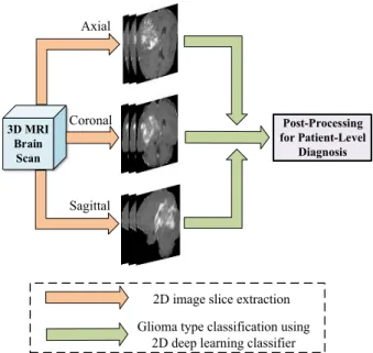
FIGURE 1. The pipeline of the proposed glioma classification scheme. The pipeline of the proposed scheme is shown in Figure1. It uses four modalities of MRIs as the inputs (T1, T1e, T2 and FLAIR). In the proposed scheme, 2D image slices are extracted from 3D volume scans in four modalities, and they are partitioned to the training, validation and testing subsets. After that, a pairwise GAN model is employed to generate synthetic MRIs for the training dataset. Real and GAN-augmented MRIs are then utilized to learn the features and the classifier for brain tumor subtypes. Finally, post-processing is conducted for the patient-level diagnosis based on majority voting of slice-level glioma subtype classification results. The main new contributions of this paper are the pairwise GANs and the patient-level-based post-processing parts, as shown in the dashed boxes. In the following, detailed descriptions on these blocks containing the main contributions will be given.

B. PAIRWISE GAN FOR MR IMAGE AUGMENTATION The pairwise GAN (Generative Adversarial Network) is employed for the augmentation of MR images. A conven-tional GAN consists of a generator and a discriminator [20]. A generator produces fake images designed to be as similar

as possible to the real images in the sense they have similar probability density distribution function. The discriminator is designed to distinguish between the real and fake images. The generator and discriminator are connected and trained iteratively in alternations through iterations to reach an opti-mal solution. The pairwise GAN uses a pair of inputs in two streams, different from conventional GAN that contains one stream of input.

1) FORMULATION OF THE PAIRWISE GAN

Let the input MR images consist ofMmodalities (M =4: T1, T1e, T2 and FLAIR in our case). Let us define the image set for them-th modality asXm= {xi,m, i=1, . . . ,Nm}, where

xi,mis thei-th 2D slice image in them-th MRI modality. Let us consider a pairwise GAN with two input streams,Xm =

{xi,m}andXn= {xi,n}, whose distributions arexi,m∼pdatam andxi,n∼pdatan, respectively. The aim of the pairwise GAN is to augment images by using a cross-modality generator and discriminator that alternatively generates synthetic (fake) images as close as possible to the real ones according to their probability distributions.

Let the generator and discriminator for them-th modality be denoted byGmandDm, respectively. In the pairwise GAN, a pair of inputs are being fed into stream-1 and stream-2 of the GAN fromm-th andn-th modality. For stream-1,Gm(·) has the inputxi,mand generates the outputxˆi,n. The discriminator

Dn(·) is to distinguish between the real and fake images (x_i,n,xˆ_i,n) in thenth modality.

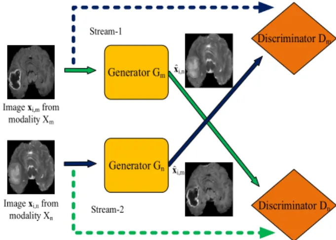
FIGURE 2. Example of the pairwise GAN model.

Conversely, for stream-2,Gn(·) has the inputxi,nand gen-eratexˆi,mas the output. The aim of the discriminatorDm(·) is to distinguish between the real and fake images (xi,m,xˆi,m) in themth modality, similar to the case in stream-1. The pairwise GAN (shown in Figure2) defines the cost function such that the two generators and discriminators are jointly optimized. These cost functions will be defined in subsequent sections.

It is worth mentioning that the proposed pairwise GAN is designed to handle two scenarios: (a) Augmenting images of fake patients (that is, to create synthetic MRIs for fake patients in order to enlarge the training dataset); (b) Aug-menting one missing modality of MR image from another

modality of MRI from a same patient (that is, when some scan modalities from a patient is missing). To deal with the first scenario (a) all existing modalities are used for aug-mentation, more synthetic MRIs can be generated through this cross-modality manner to enlarge the training dataset. These synthetic MRIs are considered as belonging to fake patients. As the original dataset contains 4 modalities of images, 6 pairs of pairwise GANs are trained for data aug-mentation (each is used for one pair of two modalities). For the second scenario (b) one pair of modalities is used, to save the computation where augmentation of one modality image is performed by choosing a best suitable modality pair, e.g. if T1 MRI is missing, T1e is used for GAN augmentation; if T2 is missing, FLAIR is selected for augmentation; if both T1 and T1e are missing, then FLAIR or T2 is used (and vice versa).

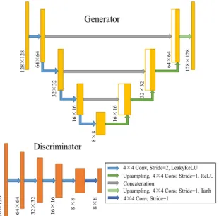
FIGURE 3. Architectures of the generator and discriminator used in the pairwise GAN. In the generator, the number of filters for each convolutional layer is set to 32, 64, 128, 256, 128, 64, 32, 1 respectively. In the discriminator, the number of filters for each convolutional layer is set to 64, 128, 256, 512, 1 respectively.

2) ARCHITECTURE OF THE PAIRWISE GAN

The architectures of the generator and discriminator are shown in Figure3. For the generator, a U-Net architecture is employed to transfer the low-level information through skip connection. The down-sampling path contains four convolu-tional layers with 4×4 filter size and stride=2. The number of filters is set to 32, 64, 128, 256 respectively, and each convolutional layer is followed by a leaky rectified linear unit (LeakyReLU) as the activation function, to introduce the non-linear characteristics to the network and generates a small positive gradient when a neuron is not active. After that, an upsampling path is employed, which consists of four convolutional layers with 4×4 filter size, stride=1 and ReLU as the activation function except Tanh is used in the last layer to generate the output image. The number of filters is set to 128, 64, 32, 1 respectively. It is worth noting that three skip-connections are used by the step concatenation, which

combines the low-level features with up-sampled high-level features for obtaining better performance. For the discrimina-tor, a Markov discriminator [21] is used to determine whether the image patches are real or fake. The least squares loss function rather than the conventional negative log likelihood is then used for obtaining stable and better training results. The discriminator consists of five convolutional layers with filter size 4×4 and the number of filters 64, 128, 256, 512, 1 respectively. The first four convolutional layers use stride

=2 and LeakyReLU, while the last one uses only stride=

1 and outputs 8×8 image patches for the discrimination. 3) LOSS FUNCTION OF THE PAIRWISE GAN

The steps for distinguishing real and fake images in then -th modality can be described as follows: first, -the generator

Gm in stream-1 usesxi,m to generate fakexˆi,n, and then the discriminatorDnin stream-2 distinguishes the fake imagexˆi,n from the real onexi,n. This can be described as firstly seeking the mapping function forGm:xi,m→ ˆxi,n.

The discriminator Dn is used to distinguish between the real and fake image, such thatDn(xi,n)≈1 for the real image, andDn(xˆi,n=Gm(xi,m))≈0, while the aim for the generator is to letDn(xˆi,n=Gm(xi,m))≈1. The adversarial loss for the

n-th modality can be described as

Ln=EXn||Dn(xi,n)−1|| 2 2+EXm ||Dn(Gm(xi,m)||22 (1) where E is the ensemble average over the dataset of the specified modality.

Similarly one may form the steps and cost functionLmfor distinguishing the real and fake images in them-th modality.

Lm=EXm||Dm(xi,m)−1|| 2 2+EXn ||Dm(Gn(xi,n)||22 (2) Since the two streams of GANs are interconnected, the loss function for the pairwise GAN can be described as:

L(Gm,Gn,Dm,Dn)=Ln+Lm+λ1L1(Gm,Gn) (3) where L1(Gm,Gn) is the loss on the generated images to measure the pixel-level difference between the fake and real images:

L1(Gm,Gn)=EXm,Xn[kMi,n(Gm(xi,m)−xi,n)k1

+kMi,m(Gn(xi,n)−xi,m)k1] (4) whereMi,mandMi,nare the tumor masks for the imagesxi,m andxi,n respectively, andis the element-wise multiplica-tion. In the mask, the intensity values are set to 1.0 and 1/3 in the tumor and the background regions respectively, in order to focus on learning tumor areas.λin (3) is the regularization parameter. The final generator and discriminator are obtained by the adversarial training based on the full loss function in (3): G∗_m,G∗_n=arg max Gm,Gn min Dm,Dn L(Gm,Gn,Dm,Dn) (5) where the discriminatorsDm, Dnand the generatorsGm, Gn are trained iteratively in alternations. For training the discrim-inators, the aim is to minimize the loss in (3) while fixing

Algorithm 1Training Process of the Pairwise GAN 1. Select two training subsetsXm,Xnof two MR

modal-ities, and sample images pairs (xi,m,xi,n) of the same patient fromXm,Xn.

2. Initialize the generators Gm, Gn and discriminators

Dm,Dn.

ForTrainingEpoch=1:Nedo:

3. Generate fake imagesGm(xi,m) andGn(xi,n) using gen-eratorsGm,Gn.

4. Compute L(Gm,Gn,Dm,Dn) and the gradient ofGm andGnusing (3);

5. Update the parameters ofGm andGnusing the gradi-ents obtained from step 4.

6. ComputeLnand the gradient ofDnusing (1);

7. Update the parameters of Dn using the gradients obtained from step 6.

8. ComputeLmand the gradient ofDmusing (2); 9. Update the parameters of Dm using the gradients

obtained from step 8. End For

Output:G∗_m,G∗_n(the latestGm,Gn)

the parameters of the generators, so that the discriminators can distinguish the synthetic images from the real ones. The generatorsGm, Gnare trained by maximizing the loss in (3) while fixing the parameters of the discriminators, in order to fool the discriminators with the synthetic images, so that the generator is able to produce synthetic images similar to the real ones.

The pairwise GANs differ from the conventional GANs in terms of its aim and the cost function. It is employed mainly for generating synthetic images across different modalities of MRIs (e.g. from FLAIR to T2, or from T2 to T1) in medical images. This also leads to a different cost function of the pairwise GAN where tumor areas are enhanced for generating synthetic MRIs. Although our choice of the generator and discriminator is similar to [21], it is worth noting that the pairwise GAN is used to train two pairs of generators and discriminators simultaneously with tumor mask added as the prior to focus on the tumor regions. It can be used to augment more training brain images considering the size of brain tumor dataset is usually not so big. Besides, missing MRI scans in some modalities in datasets is a very common and practical issue, the pairwise GAN is thus able to generate synthetic data in these missing modalities.

4) TRAINING PROCESS OF THE PAIRWISE GAN

The training process for the pairwise GAN is shown in the following algorithm where the generators and the discrimi-nators are updated in alternation until the maximum training epoch is reached. After the training process, two genera-tors G∗_m andG∗_nare used for synthesizing MRIs across two modalities.

FIGURE 4. Illustration on post-processing for patient-level diagnosis.

C. POST-PROCESSING FOR PATIENT-LEVEL DIAGNOSIS BASED ON 3D VOLUME IMAGES

Since the number of 3D brain volume images in a dataset is moderate, 2D brain image slices are used as this leads to more training data. This also leads to reduced dimensionality of the input data (noting that a high dimensional input is subjected to ‘‘the curse of dimensionality’’), hence it can mitigate the overfitting in the training process. In the proposed scheme, 2D MRI slices are extracted from three different views (axial, coronal, sagittal) in each modality, which increases the diver-sity of input 2D MRI slices and prevents the network from overfitting to specific image views.

As the 2D image-based classifier outputs the glioma sub-type for each image slice, it is necessary to make a patient-level decision based on all slice prediction results for each individual patient. Since the output subtypes from the 2D image-based classifier can be different for different slices from a same patient, due to variations of slices and image view angles, it is hence necessary to introduce a post-processing approach in order to obtain a consistent predic-tion of the glioma subtype for each patient based on the corresponding 3D scan. We propose a majority voting-based criterion for making the final tumor subtype classification on each patient, as depicted in Figure4. That is, the final diagnosis of a patient is determined by the majority classi-fication results from all corresponding slices of a patient. Let

si, (i=1,· · · ,N) be theith slice prediction result of glioma subtype,Nis the total number of extracted tumor image slices of a patient,si = 1 if the slice belongs to IDH1 mutation, andsi=0 if it belongs to IDH1 wild-type. The final glioma subtype prediction resultsfor this patient is determined by

s= ( 1 XN i=1si>N/2 0 otherwise (6)

D. IMPLEMENTATION ISSUES

1) REVIEW OF MULTI-STREAM 2D CONVOLUTIONAL NEURAL NETWORKS

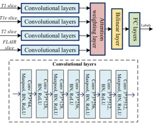
For the sake of convenience to the readers, the multi-stream 2D slice-based CNN feature extraction and classification scheme [24] is briefly reviewed. The multi-stream 2D CNN architecture consists of four separate streams for learning glioma features from four modalities of MR images followed by modality-level feature fusion, as shown in Figure5.

FIGURE 5. The pipeline of the baseline multi-stream 2D convolutional network architecture for glioma subtype classification. BN: batch normalization.

For each stream, MR images from a single modality are used as the input, where multi-stream CNNs form a set of parallel independent CNN networks. In such a way, modality-specific features are learned through each individual CNN stream.

The CNN architecture for each stream consists of seven layers, that is carefully selected after numerous empirical tests. Filter of size 3*3 is used in each layer, similar to the filter settings used in the VGG net [25]. Four feature maps are then extracted from the final convolutional layer (i.e., 7th layer) in the four streams and fed to the next layer for feature fusion and refinement.

Observing that features from different modalities con-tribute differently and complement each other, we introduce a different fusion strategy, namely, attention-weighted fusion strategy as compared with that in [24]. As shown schemati-cally in Figure5, we apply weighted sum on these features, so that the weights can be are learned adaptively according to features in each modality. LetFi, i = 1,· · · ,4, be the feature maps from four modalities in the final convolutional layer, then the combined feature matrix F is formed as F=P4

i=1 aiFi, where the weightakis defined by

ak=

exp(wT_kfk)

P4

i=1exp(wTifi)

(7)

where wk is a column-scanned vector of Wk, Wk is the attention weighting matrix forkth modality of features,akis

the softmax-normalized attention weight for the feature vec-tor fk, fk is a column-scanned vector of Fk. For the fea-ture fusion, the attention weighting matrix Wk is learned adaptively according to the characteristics of features from different modalities.

For the refinement of fused features, a bilinear layer similar to [26], is then employed that maps the fused features to a high dimensional feature space. The refined feature map is obtained by exploiting the interactions of fused features at different spatial locations asH=(F0)TF0, whereF0∈_Rhw∗c

is reshaped from the fused feature map F ∈ _Rh∗w∗c, and

h, w, care the height, width and the number of channels in F, respectively. The bilinear layer leads to a high-dimensional feature representation that contains complementary features from different modalities. After the feature refinement in the bilinear layer, the refined feature mapHis then fed to the clas-sifier. The classifier consists of three fully-connected layers where the number of neurons is 256, 256, 2, respectively.

2) A TWO-STAGE TRAINING STRATEGY WITH AN END-TO-END TRAINING

For effectively training the networks, we propose a two-stage training strategy, where the augmented and real images are treated separately instead of mixing them during the training. This is based on the observation that distributions from GAN-augmented MRIs still present some differences from the real ones. Hence, a two-stage training strategy is adopted, aimed at learning generic features and fast convergence by applying initial training from augmented MRIs, followed by refined feature learning from real MRIs. The two-stage training is performed as follows: the augmented images are used initially for pre-training the whole network for glioma subtype feature learning and classification, and then the real MRI data is used for refined-training. This has led to some performance improvement as have been noticed from our empirical tests. Furthermore, this baseline scheme of multi-stream CNN fea-ture extraction and glioma subtype classification is able to be trained end-to-end.

III. EXPERIMENTS AND RESULTS A. SETUP, DATASETS, AND METRICS

1) SETUP

KERAS library [27] with TensorFlow [28] backend was used for our experiments. All experiments were conducted on a workstation with Intel-i7 3.40GHz CPU, 48G RAM and a NVIDIA Titan XP 12GB GPU. The commonly used cri-teria on the overall accuracy and cross-entropy loss were used for the performance evaluation. The size of the input image slice was 128*128. Class-weight was set to 2 for the class IDH1 mutation and 1 for the class IDH1 wild-type in the multi-stream CNN training, since the number of samples in the IDH1 mutation class was about half in that of IDH1 wild-type class. For the pairwise GAN, 1000 epochs were used for the training, where the learning rate was set to 0.0002 with an Adam optimizer. For the multi-stream

CNN pre-training, the number of epochs was set to 100, the optimizer Adagrad was used, and a step-wise learning rate was set, i.e., to 0.0001 for epochs∈[1, 30], 0.00001 for epochs ∈ [31, 60], and 0.000001 for epochs ∈ [61, 100]. For refined training of multi-stream CNNs, the learning rate was set to 0.000001 using 50 epochs. Early stopping strat-egy was adopted during the CNN training process, where parameters of the network were fixed from a certain epoch when a best validation performance was achieved. Simple data augmentation approaches were used as well, including random horizontal flipping and shifting (maximum 10% of width and height). They were performed only on the training dataset in real time to minimize the memory usage.

2) DATASET

The dataset used in our experiments contains 3D brain vol-ume images from TCGA-GBM [29] and TCGA-LGG [30]. In the dataset, the MR images of each patient consist of four modalities (T1, T1e, T2, FLAIR), the tumor segmen-tation results, as well as the corresponding molecular-based IDH1 genotype labels as the tumor subtypes.

TABLE 1. (a) Dataset information. Females/males: F/M, Four age groups were included: ([<30 )/ [30,60) / [60,80) /[≥80]). Noting that one patient of IDH1 wild-type in the dataset lacks age and gender information. (b) Partitioned dataset.

Detailed information of the dataset is given in Table1(a). Observing that the volume of tumor is usually small/medium in size, six slices that contain glioma were extracted from each individual scan. This was done for both classes. For the focused feature learning on the tumor areas instead of the whole brain, tumor masks were applied to enhance the tumor feature learning similar to [24]. For our experiments, the dataset was partitioned into 3 subsets: training, valida-tion and testing, detailed informavalida-tion is shown in Table1(b). All 2D image slices in these 3 subsets were partitioned according to patients, i.e., images from the same patient were kept together in either training subset or the testing subset, as such partition is clinically important.

We define 2 case studies, Case-A is for enlarged train-ing dataset containtrain-ing fake patients, Case-B is for enlarged training dataset including augmentation of both fake patients and missing scans from some modalities. For Case-A study, the training dataset was formed by the combination of (S1+S2), for Case-B study, the training dataset was formed by the combination of (S3+S4+S5), as shown in Figure6.

FIGURE 6.Enlarged training datasets in two case studies formed from the dataset, where shaded bar areas are GAN-augmented images. In Case-A, the training dataset was formed by the combination of (S1+S2), adding synthesized MRIs of fake patients; and in Case-B, the training dataset was formed by the combination of (S3+S4+S5), adding synthesized MRIs from missing modalities and enlarging the training dataset by adding synthesized MRIs of fake patients.

In Case-A and Case-B studies, S1-S5 are defined as follows:

S1: A subset of original training MR images from all modal-ities (i.e., 60% MRIs from the dataset in Table1); S2: A subset of GAN-generated synthetic MRIs for all

modalities, which was equivalent to generating synthetic MRIs for fake patients. This subset consisted of 297 fake patients with 1782 MRIs.

S3: A subset of original training MRIs in (S1) minus 24% of MRIs from four scanner modalities, where 6% of patients’ images were removed in each modality; S4: A subset of GAN-generated synthetic MRIs that were

used to replace the missing 24% MRIs in (S3);

S5: A subset of GAN-generated synthetic MRIs for fake patients in four modalities. It consisted of a total of 225 fake patients with 1350 MRIs.

3) METRICS FOR PERFORMANCE EVALUATION

Objective metrics were used to evaluate the performance of the glioma classification, based on the following four kinds of samples.

True positive: the IDH1 mutation glioma, and was cor-rectly classified as the IDH1 mutation.

False positive: the IDH1 wild-type glioma, but was incor-rectly classified as the IDH1 mutation.

True negative: the IDH1 wild-type glioma, and was cor-rectly classified as the IDH1 wild-type.

False negative: the IDH1 mutation glioma, but was incor-rectly classified as the IDH1 wild-type.

Let TP, FP, TN and FN be the number of true positives, false positives, true negatives and false negatives, the three metrics overall accuracy, sensitivity and specificity were defined as follows respectively: Accuracy = TP+TN TP+FP+TN+FN Sensitivity= TP TP+FN, Specificity= TN FP+TN

B. PERFORMANCE OF THE PROPOSED METHOD: 2 CASE STUDIES

To test the effectiveness of the proposed method for classi-fying the glioma subtype IDH1 mutation, experiments were conducted with 5 runs, where the partitions of training, val-idation and test subsets in the dataset were done randomly in each of the 5 runs. Table2shows the performance of the 5 runs as well as the average performance based on testing accuracy, sensitivity and specificity after the post-processing for patient-level diagnosis based on 3D volume images.

TABLE 2. Overall performance, sensitivity and specificity of the proposed method for Case-A and Case-B studies on the testing set in the 5 runs. For each run, the training/validation/test subsets were randomly

re-partitioned according to the patients. Result is shown in mean value(standard deviation|σ|). Prop-A: the proposed method on Case-A, Prop-B: the proposed method on Case-B. Acc: accuracy, sen: sensitivity, spe: specificity.

Observing Table 2, the proposed method is shown to be effective on the testing dataset. For Case-A study, a relatively high averaging classification accuracy 88.82% was achieved in 5 runs (|σ| = 6.37%), with a sensitivity value 81.81% (|σ| =11.13%) and specificity value 92.17% (|σ| =4.77%). For Case-B study, averaging classification accuracy was 88.23%, with a sensitivity value 79.99% (|σ| =14.94%) and specificity value 92.17% (|σ| =4.77%). Further comparing with the results on A and B, one can see that Case-B has a slightly reduced accuracy (−0.59%) and sensitivity (−1.82%) and a similar specificity value on the average of 5 runs. This slightly reduced performance is expected as Case-B also included missing scanner modalities in some patients’ training data.

C. VISUAL EXAMPLES OF CROSS-MODALITY MRI AUGMENTATION FROM PAIRWISE-GANS

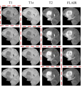
The pairwise GAN is shown to work well both empiri-cally, and from visual observations of randomly selected augmented MR images, where the augmented brain MRIs seem to closely resemble the real ones containing tumors. Some cross-modality synthetic image examples generated by the pairwise GANs are shown in Figure 7, where each row contains the real MRI (in red box) and the remaining 3 augmented MRIs in different modalities (e.g., T1, T1e, T2, or FLAIR).

Observing Figure 7, the augmented images are of good quality, and look rather similar to the real ones. Although the distributions could still be somewhat different from the real images.

We also randomly picked up a small percentage of GAN-generated images, and provided them to a radiologist, who considered them highly resemble the real brain images with glioma. It is worth mentioning that the GAN-generated

FIGURE 7. Examples of pairwise GAN-augmented synthetic images from the dataset. In the figure, four columns of images correspond to four different modalities of T1, T1e, T2 and FLAIR, while each row contains one real image (in red box) and three synthetic ones generated from this real image.

data was used for generic feature learning in the pre-training stage, while the refined training used the real MRIs for learn-ing more specific features of gliomas.

D. IMPROVED TESTING PERFORMANCE OF CLASSIFIERS TRAINED BY ENLARGED DATASETS WITH REAL AND AUGMENTED MRIS

1) COMPARISON OF THE PROPOSED METHOD ON CASE-A WITH BASELINE-1 METHOD

In this set of experiments, we evaluate the impact of adding synthetic MRIs of fake patients to the training dataset. The proposed method was tested using the enlarged training dataset by combining (S1 +S2). We then compared our proposed method with the 1 method. The baseline-1 method was defined the same as the multi-stream 2D CNN followed by post-processing, however, the training dataset only consisted of the real MRIs, i.e., (S1). Table3 shows the glioma classification results on the testing set, including the overall performance, sensitivity and specificity on the testing set, both for the proposed method and the baseline method.

Observing Case-A results in Table3, one can see that the proposed method has obtained improved the accuracy on the test set (average 88.82%, about 2.94% improvement over the baseline-1 method), with a slightly increased standard deviation (3.15%) indicating more variance in the estimation. The results have also shown an increased sensitivity (aver-age 81.81% about 12.73% improvement over the baseline-1 method) indicating increased positive classification rate, and slightly decreased specificity (average 92.17% about 1.74% lower) indicating a slightly more increase on false alarm.

TABLE 3. Test results on the dataset in the 5 runs from the proposed method where the enlarged training dataset consisted of (S1)+(S2); and from the baseline-1 method where the training dataset only consisted of (S1). Both the baseline and proposed method use multi-stream 2D CNNs for glioma classification followed by post-processing. For each run, the training, validation and testing subsets were randomly re-partitioned according to the patients. The mean value and standard deviation|σ|

were also included. Prop-A: the proposed method on Case-A, Bas-1: baseline-1 method, STD: standard deviation.

2) COMPARISON OF THE PROPOSED METHOD ON CASE-B WITH BASELINE-2 METHOD

In this set of experiments, we evaluate the impact of adding synthetic MRIs from missing modalities and from fake patients. The proposed method was then tested using the above training data combination (S3 + S4 + S5). The baseline-2 method was defined the same as the multi-stream 2D CNN followed by post-processing, however, the training dataset only consisted of real MRIs, i.e., (S3). Table4shows the glioma classification results on accuracy, sensitivity and specificity from the testing set.

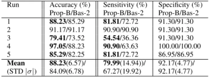
TABLE 4. Test results on the dataset in the 5 runs from the proposed method where the training dataset consisted of (S3+S4+S5); and from the baseline-2 method where the training dataset only consisted of (S3). Both the baseline and proposed method use 2D multi-stream CNNs for glioma classification followed by post-processing. For each run, the training, validation and testing subsets were randomly re-partitioned according to the patients. The mean value and standard deviation|σ|

were also included. Prop-B: the proposed method on Case-B, Bas-2: baseline-2 method, STD: standard deviation.

Observing Case-B results in Table 4, one can see that the proposed method has obtained improved accuracy on the test set (average 88.23%, about 4.14% improvement over the baseline-2 method), with improved sensitivity (aver-age 79.99% about 12.72% improvement over the baseline-2 method) indicating an improved positive classification rate, and same specificity 92.17% as compared with the baseline-2 method.

E. EVALUATION OF TUMOR MASK IN GLIOMA

CLASSIFICATION AND GAN-BASED MRI AUGMENTATION

1) EFFECT OF MASKS FOR CLASSIFIER

To examine the effect of tumor masks for glioma classifica-tion, a comparison was made on the proposed method using

TABLE 5.Test accuracy for overall classification performance, sensitivity and specificity from different methods: with and without tumor mask enhancement. Results of 5 runs are shown in mean value (standard deviation|σ|). Acc: accuracy, sen: sensitivity, spe: specificity.

MRIs with and without tumor mask enhancement. Table5

shows the comparison on accuracy, sensitivity and specificity from the proposed method on the testing set.

Observing Table5, the proposed method using tumor mask enhancement has led to improved classification accuracy (by 7.67%), with much higher sensitivity rate and specificity rate. This also indicates that tumor mask enhancement has led to better glioma classification performance on IDH1 mutation subtype and more balanced results on two subtype classes. 2) EFFECT OF MASKS ON AUGMENTED DATA

To examine the effect of tumor masks on GAN-augmented data, comparisons were made on pairwise GAN generated images with and without tumor mask enhancement. The augmented images were then compared with the real MRIs by using peak signal-to-noise ratio. In addition, the images were projected to the latent feature space by convolutional autoencoder similar to [16]. The encoder had 8 convolutional layers with 3*3 filter size. The number of filters was set to 64, 64, 128, 128, 256, 256, 512 and 512 respectively, and the stride was set to 2 every other layer. The decoder had a reverse structure of the encoder and each convolution was replaced by deconvolution. The input image size was 128*128*4 where 4 modalities were stacked together. The latent feature vector with dimensionality 512 was obtained from the globally max pooled feature map of the last convolutional layer in the decoder. The Euclidean distance between centroids of the feature space was applied to compare the real and GAN-augmented images from methods with and without tumor mask enhancement. Table 6 shows the comparison on two metrics, peak signal-to-noise ratio (PSNR) and the distance to the real images based on autoencoder features (DAEF), on the whole image and on the tumor region only.

TABLE 6.Comparison of real and generated MRIs using peak signal-to-noise ratio (PSNR) and distance to the real images based on autoencoder features (DAEF) from methods with and without tumor mask enhancement. The larger the value of PSNR, the better the performance. The smaller the value of DAEF, the better the performance. Results of 5 runs are shown in mean value (standard deviation|σ|).

Observing Table6, the proposed method using tumor mask enhancement has led to higher PSNR on the tumor region, although on the whole image PSNR of the method without

mask was higher. It indicated that the proposed pairwise GAN with tumor mask enhancement was able to generate more precise tumor regions. DAEF results in Table6showed that the method with mask had the encoded feature closer to that of real images both on the whole image and on the tumor region. It is worth noting that the comparison on the augmented data only gave indications since the two metrics used here did not reflect the image quality from the molecular level.

F. COMPARISONS WITH STATE-OF-THE-ART METHODS Comparisons were made with existing methods for classify-ing gliomas subtypes with IDH1 mutation/wild-type. Results are shown in Table 7. It is worth emphasizing that these comparisons can only be used as an indication as the datasets used in these methods were different, with exception of the method [15] in Table7.

TABLE 7. Comparison of the proposed method with 4 existing methods for glioma subtype IDH1 mutation/wild-type classification. It is worth noting that only [15] used the same dataset as ours, and the other results listed in the table can only be used as a performance indication.

Observing Table7, the proposed method was comparable to others, indicating relatively good performance. The pro-posed method achieved a better result than [15] on the same dataset. Other methods [10], [11], [14] only give indications on relative performance due to using different datasets, which also indicated that the proposed scheme has the performance comparable to the state-of-the-art.

G. DISCUSSIONS

From different sets of experimental results described above, the following insights may be gained on the proposed scheme:

• Overall performance: The proposed scheme is effective, with an excellent classification performance of glioma subtypes (88.82% on the testing set);

• Training the proposed scheme by enlarged datasets with real+pairwise GAN augmented MRIs across different modalities from fake patients has led to improved clas-sification performance (increased 2.94%) on the testing set for glioma subtypes of IDH1 mutation/wild-type. This indicates that the pairwise GAN is robust and effec-tive, and can be used as a tool for enlarging the training dataset with mixed real and augmented data with further enhanced generalization performance of glioma subtype classification;

• Tumor masks are effective for glioma subtype classifi-cation and GAN-based MRI augmentation. They lead to an increase of classification performance by 7.67%,

and more precise tumor regions in the GAN augmented images.

Future work includes applying multiple datasets with cross-domain cross-modality GAN data augmentation, clas-sifying gliomas with additional subtypes of 1p/19q codeletion classes which are important to glioma prognosis, and incorpo-rating patient side information (e.g. ages, survival years), for predicting more glioma subtypes as well as patient survival. IV. CONCLUSION

The proposed scheme has been tested using real and pairwise GAN-augmented MRIs as training data, results obtained on the testing dataset have demonstrated that the scheme is effec-tive and robust (average 88.82% test accuracy for gliomas subtypes of IDH1 mutation/wild-type). Using two enlarged datasets containing real and GAN-augmented MRIs for train-ing the proposed scheme, has both resulted in increased gen-eralization performance of the classifier on the testing set. This indicates that the proposed pairwise GAN is effective and robust, and is useful for augmenting MRIs when the size of brain tumor training dataset is not sufficiently large for deep learning. The post-processing step is essential for diag-nosis based on 3D volume images, and the two-stage training strategy is useful for real and GAN-augmented MRIs. Finally, comparisons with several existing methods, though based on different datasets, have indicated that the proposed scheme using mixed real and GAN-augmented training datasets has reached comparable performance to the state-of-the-art. ACKNOWLEDGMENT

The results were based upon data generated by the TCGA Research Network: https://www.cancer.gov/tcga. All work related to this paper was conducted at Chalmers University of Technology.

REFERENCES

[1] S. Cha, ‘‘Update on brain tumor imaging: From anatomy to physiology,’’ Amer. J. Neuroradiol., vol. 27, no. 3, pp. 475–487, 2006.

[2] J. Uhm, ‘‘An integrated genomic analysis of human glioblastoma multi-forme,’’Yearbook Neurol. Neurosurg., vol. 2009, pp. 115–116, Jan. 2009. [3] J. E. Eckel-Passow and D. H. Lachance, ‘‘Glioma groups based on 1p/19q, IDH, and TERT promoter mutations in tumors,’’New England J. Med., vol. 372, no. 26, pp. 2499–2508, 2015.

[4] C. Hartmann, B. Hentschel, W. Wick, D. Capper, J. Felsberg, M. Simon, M. Westphal, G. Schackert, R. Meyermann, T. Pietsch, G. Reifenberger, M. Weller, M. Loeffler, and A. Von Deimling, ‘‘Patients withIDH1 wild type anaplastic astrocytomas exhibit worse prognosis thanIDH1-mutated glioblastomas, andIDH1 mutation status accounts for the unfavorable prognostic effect of higher age: Implications for classification of gliomas,’’ Acta Neuropathol., vol. 120, no. 6, pp. 707–718, Dec. 2010.

[5] C. Houillier, X. Wang, G. Kaloshi, K. Mokhtari, R. Guillevin, J. Laffaire, S. Paris, B. Boisselier, A. Idbaih, F. Laigle-Donadey, K. Hoang-Xuan, M. Sanson, and J.-Y. Delattre, ‘‘IDH1 orIDH2 mutations predict longer survival and response to temozolomide in low-grade gliomas,’’Neurology, vol. 75, no. 17, pp. 1560–1566, Oct. 2010.

[6] J. Uhm, ‘‘IDH1 andIDH2 mutations in gliomas,’’Yearbook Neurol. Neurosurg., vol. 2009, pp. 119–120, Jan. 2009.

[7] Y. Kang, S. H. Choi, Y.-J. Kim, K. G. Kim, C.-H. Sohn, J.-H. Kim, T. J. Yun, and K.-H. Chang, ‘‘Gliomas: Histogram analysis of apparent dif-fusion coefficient maps with standard- or high-b-value difdif-fusion-weighted MR imaging—Correlation with tumor grade,’’Radiology, vol. 261, no. 3, pp. 882–890, Dec. 2011.

[8] J. Carrillo and A. Lai, ‘‘Relationship between tumor enhancement, edema, IDH1 mutational status, MGMT promoter methylation, and survival in glioblastoma,’’Amer. J. Neuroradiol., vol. 33, no. 7, pp. 1349–1355, 2012. [9] S. Qi, L. Yu, H. Li, Y. Ou, X. Qiu, Y. Ding, H. Han, and X. Zhang, ‘‘Isocitrate dehydrogenase mutation is associated with tumor location and magnetic resonance imaging characteristics in astrocytic neoplasms,’’ Oncol. Lett., vol. 7, no. 6, pp. 1895–1902, Jun. 2014.

[10] J. Yu, Z. Shi, Y. Lian, Z. Li, T. Liu, Y. Gao, Y. Wang, L. Chen, and Y. Mao, ‘‘NoninvasiveIDH1 mutation estimation based on a quantitative radiomics approach for grade II glioma,’’Eur. Radiol., vol. 27, no. 8, pp. 3509–3522, Aug. 2017.

[11] X. Zhang, Q. Tian, L. Wang, Y. Liu, B. Li, Z. Liang, P. Gao, K. Zheng, B. Zhao, and H. Lu, ‘‘Radiomics strategy for molecular subtype stratifi-cation of lower-grade glioma: Detecting IDH and TP53 mutations based on multimodal MRI,’’J. Magn. Reson. Imag., vol. 48, no. 4, pp. 916–926, Oct. 2018.

[12] B. Shofty, M. Artzi, D. B. Bashat, G. Liberman, O. Haim, A. Kashanian, F. Bokstein, D. T. Blumenthal, Z. Ram, and T. Shahar, ‘‘MRI radiomics analysis of molecular alterations in low-grade gliomas,’’Int. J. Comput. Assist. Radiol. Surg., vol. 13, no. 4, pp. 563–571, Apr. 2018.

[13] Z. Li, Y. Wang, and J. Yu, ‘‘Deep learning based radiomics (DLR) and its usage in noninvasiveIDH1 prediction for low grade glioma,’’Sci. Rep., vol. 7, no. 1, 2017, Art. no. 5467.

[14] K. Chang, H. X. Bai, H. Zhou, and C. Su, ‘‘Residual convolutional neural network for the determination of IDH status in low-and high-grade gliomas from MR imaging,’’Clin. Cancer Res., vol. 24, no. 5, pp. 1073–1081, 2018. [15] S. Liang, R. Zhang, D. Liang, T. Song, T. Ai, C. Xia, L. Xia, and Y. Wang, ‘‘Multimodal 3D DenseNet for IDH genotype prediction in gliomas,’’ Genes, vol. 9, no. 8, p. 382, Jul. 2018.

[16] H. Salehinejad, E. Colak, T. Dowdell, J. Barfett, and S. Valaee, ‘‘Synthe-sizing chest X-ray pathology for training deep convolutional neural net-works,’’IEEE Trans. Med. Imag., vol. 38, no. 5, pp. 1197–1206, May 2019. [17] H. Salehinejad, S. Valaee, T. Dowdell, E. Colak, and J. Barfett, ‘‘General-ization of deep neural networks for chest pathology classification in X-rays using generative adversarial networks,’’ inProc. IEEE Int. Conf. Acoust., Speech Signal Process. (ICASSP), Apr. 2018, pp. 990–994.

[18] D. Korkinof, T. Rijken, M. O’Neill, J. Yearsley, H. Harvey, and B. Glocker, ‘‘High-resolution mammogram synthesis using progressive generative adversarial networks,’’ 2018, arXiv:1807.03401. [Online]. Available: https://arxiv.org/abs/1807.03401

[19] A. Gupta, S. Venkatesh, S. Chopra, and C. Ledig, ‘‘Generative image translation for data augmentation of bone lesion pathology,’’ 2019, arXiv:1902.02248. [Online]. Available: https://arxiv.org/abs/1902.02248 [20] I. Goodfellow, ‘‘Generative adversarial nets,’’ inProc. Adv. Neural Inf.

Process. Syst., 2014, pp. 2672–2680.

[21] P. Isola, J.-Y. Zhu, T. Zhou, and A. A. Efros, ‘‘Image-to-image translation with conditional adversarial networks,’’ inProc. IEEE Conf. Comput. Vis. Pattern Recognit. (CVPR), Jul. 2017, pp. 5967–5976.

[22] J.-Y. Zhu, T. Park, P. Isola, and A. A. Efros, ‘‘Unpaired image-to-image translation using cycle-consistent adversarial networks,’’ inProc. IEEE Int. Conf. Comput. Vis. (ICCV), Oct. 2017, pp. 2223–2232.

[23] M. Y. Liu, T. Breuel, and J. Kautz, ‘‘Unsupervised image-to-image transla-tion networks,’’ inProc. Adv. Neural Inf. Process. Syst., 2017, pp. 700–708. [24] C. Ge, I. Y.-H. Gu, A. S. Jakola, and J. Yang, ‘‘Deep learning and multi-sensor fusion for glioma classification using multistream 2D convolutional networks,’’ inProc. 40th Annu. Int. Conf. IEEE Eng. Med. Biol. Soc. (EMBC), Jul. 2018, pp. 5894–5897.

[25] K. Simonyan and A. Zisserman, ‘‘Very deep convolutional networks for large-scale image recognition,’’ 2014,arXiv:1409.1556. [Online]. Avail-able: https://arxiv.org/abs/1409.1556

[26] A. Diba, V. Sharma, and L. V. Gool, ‘‘Deep temporal linear encoding networks,’’ inProc. IEEE Conf. Comput. Vis. Pattern Recognit. (CVPR), vol. 1, Jul. 2017, pp. 2329–2338.

[27] F. Chollet. (2015). Keras. [Online]. Available: https://github.com/ fchollet/keras

[28] M. Abadi and A. Agarwal.TensorFlow: Large-Scale Machine Learning on Heterogeneous Systems. [Online]. Available: http://tensorflow.org [29] S. Bakas, H. Akbari, and H. Sotiras, ‘‘Segmentation labels and radiomic

features for the pre-operative scans of the TCGA-GBM collection,’’ Tech. Rep., 2017, doi:10.7937/K9/TCIA.2017.KLXWJJ1Q.

[30] S. Bakas, H. Akbari, and H. Sotiras, ‘‘Segmentation labels and radiomic features for the pre-operative scans of the TCGA-LGG collection,’’ Tech. Rep., 2017, doi:10.7937/K9/TCIA.2017.GJQ7R0EF.

CHENJIE GE(Student Member, IEEE) received the bachelor’s degree from the Harbin Institute of Technology, China, in 2013. He is currently pur-suing the dual Ph.D. degree with the Department of Electrical Engineering, Chalmers University of Technology, Sweden, and the Institute of Image Processing and Pattern Recognition, Shanghai Jiao Tong University, China. His research interests are computer vision, image processing, machine learning, and deep learning, with applications to medical image analysis, human activity classification, and visual saliency detection.

IRENE YU-HUA GU (Senior Member, IEEE) received the Ph.D. degree in electrical engineer-ing from the Eindhoven University of Technology, Eindhoven, The Netherlands, in 1992.

From 1992 to 1996, she was a Research Fel-low with the Philips Research Institute IPO, Eind-hoven, held a postdoctoral position at Staffordshire University, Staffordshire, U.K., and a Lecturer with the University of Birmingham, Birmingham, U.K. She has been with the Department of Signals and Systems, Chalmers University of Technology, Gothenburg, Sweden, since 1996, where she has been a Full Professor, since 2004. Her research interests include statistical image and video processing, object tracking and video surveillance, machine learning and deep learning, and signal process-ing with applications to electric power systems. She was the Chair-Elect of the IEEE Swedish Signal Processing Chapter, from 2001 to 2004. She was an Associate Editor for the IEEE TRANSACTIONS ONSYSTEMS, MAN, AND CYBERNETICS, PARTA: SYSTEMS ANDHUMANS, and PARTB: CYBERNETICS,from 2000 to 2005, and an Associate Editor for theEURASIP Journal on Advances in Signal Processing, from 2005 to 2016, and Editorial Board of theJournal of Ambient Intelligence and Smart Environments, from 2011 to 2019.

ASGEIR STORE JAKOLA received the Ph.D. degree in medicine from the Norwegian University of Science and Technology, Trondheim, Norway, in 2013.

He has been a Medical Doctor, since 2006. He is a clinically active Neurosurgeon with a special interest in brain tumor research, medical technol-ogy, and clinical research with the fields of neu-rology, neurosurgery, and oncology. He was with Sahlgrenska Academy, Institution of Neuroscience and Physiology, Gothenburg, Sweden, as an Adjunct Lecturer, in 2015, and has been an Associate Professor, since 2016. Since 2015, he has been an Editorial Board Member inActa Neuroschirurgica, and he was elected as an Executive Board Member of EANO, in 2018.

JIE YANG (Member, IEEE) received the Ph.D. degree from the Department of Computer Sci-ence, Hamburg University, Hamburg, Germany, in 1994.

He is currently a Professor with the Institute of Image Processing and Pattern Recognition, Shang-hai Jiao Tong University, ShangShang-hai, China. He has led many research projects, had one book pub-lished in Germany, and authored over 200 jour-nal articles. His current research interests include object detection and recognition, data fusion and data mining, and medical image processing.