Kernel Machine Methods for Risk Prediction with High Dimensional
Data
(Article begins on next page)
The Harvard community has made this article openly available.
Please share
how this access benefits you. Your story matters.
Citation
No citation.
Accessed
February 19, 2015 10:34:18 AM EST
Citable Link
http://nrs.harvard.edu/urn-3:HUL.InstRepos:9793867
Terms of Use
This article was downloaded from Harvard University's DASH
repository, and is made available under the terms and conditions
applicable to Other Posted Material, as set forth at
http://nrs.harvard.edu/urn-3:HUL.InstRepos:dash.current.terms-of-use#LAA
Kernel Machine Methods for Risk Prediction with High
Dimensional Data
A dissertation presented
by
Jennifer Anne Sinnott
to
The Department of Biostatistics
in partial fulfillment of the requirements
for the degree of
Doctor of Philosophy
in the subject of
Biostatistics
Harvard University
Cambridge, Massachusetts
August 2012
c
�2012 - Jennifer Anne Sinnott All rights reserved.
Dissertation Advisor: Professor Tianxi Cai Jennifer Anne Sinnott
Kernel Machine Methods for Risk Prediction with High Dimensional Data
Abstract
Understanding the relationship between genomic markers and complex disease could have a pro-found impact on medicine, but the large number of potential markers can make it hard to differentiate true biological signal from noise and false positive associations.
A standard approach for relating genetic markers to complex disease is to test each marker for its association with disease outcome by comparing disease cases to healthy controls. It would be cost-effective to use control groups across studies of many different diseases; however, this can be problematic when the controls are genotyped on a platform different from the one used for cases. Since different platforms genotype different SNPs, imputation is needed to provide full genomic coverage, but introduces differential measurement error. In Chapter 1, we consider the effects of this differential error on association tests. We quantify the inflation in Type I Error by comparing two healthy control groups drawn from the same cohort study but genotyped on different platforms, and assess several methods for mitigating this error.
Analyzing genomic data one marker at a time can effectively identify associations, but the resulting lists of significant SNPs or differentially expressed genes can be hard to interpret. Integrating prior biolog-ical knowledge into risk prediction with such data by grouping genomic features into pathways reduces the dimensionality of the problem and could improve models by making them more biologically grounded and interpretable. The kernel machine framework has been proposed to model pathway effects because it allows nonlinear associations between the genes in a pathway and disease risk. In Chapter 2, we propose kernel machine regression under the accelerated failure time model. We derive a pseudo-score statistic for testing and a risk score for prediction using genes in a single pathway. We propose omnibus procedures that alleviate the need to prespecify the kernel and allow the data to drive the complexity of the resulting model. In Chapter 3, we extend methods for risk prediction using a single pathway to methods for risk prediction model using multiple pathways using a multiple kernel learning approach to select important pathways and efficiently combine information across pathways.
Contents
Title page . . . i Abstract . . . iii Table of Contents . . . iv Contents iv Acknowledgments . . . vi1 Artifact due to differential error when cases and controls are imputed from different platforms 1 1.1 Introduction . . . 3 1.2 Methods . . . 5 1.2.1 Method 1 . . . 7 1.2.2 Method 2 . . . 7 1.2.3 Method 3 . . . 8 1.3 Results . . . 8 1.3.1 Method 1 . . . 10 1.3.2 Method 2 . . . 10 1.3.3 Method 3 . . . 12 1.4 Discussion . . . 15
2 Omnibus Risk Assessment via Accelerated Failure Time Kernel Machine Modeling 19 2.1 Introduction . . . 21
2.2 The Kernel Machine Accelerated Failure Time Model . . . 23
2.3.1 The Pseudo-Score Statistic . . . 25
2.3.2 Approximating the Null Distribution of the Score Statistic . . . 26
2.3.3 Estimation and the Kernel Principal Components Analysis Approximation . . . 27
2.4 General WLR and Kernel Selection . . . 28
2.4.1 Testing and Prediction with General Weights . . . 28
2.4.2 Combining P-Values Across Models and Kernels . . . 29
2.5 Simulation Studies . . . 30
2.5.1 Testing . . . 30
2.5.2 Estimation . . . 35
2.6 Example: Breast Cancer Gene Expression Study . . . 35
2.7 Discussion . . . 40
2.8 Appendix: Asymptotic Distribution of the Test Statistic . . . 41
3 Pathway Selection and Aggregation using Multiple Kernel Learning for Risk Prediction 45 3.1 Introduction . . . 47
3.2 Approach with a General Objective Function . . . 48
3.2.1 Kernel Machine Modeling . . . 48
3.2.2 Kernel PCA . . . 50
3.2.3 Least Squares Approximation . . . 51
3.2.4 Kernel Selection and Tuning . . . 51
3.2.5 Pathway Screening . . . 53
3.3 Examples . . . 53
3.3.1 Cox Model . . . 53
3.3.2 AFT model . . . 53
3.4 Simulation Studies . . . 54
3.5 Example: Breast Cancer Gene Expression Study . . . 56
3.6 Discussion . . . 58
3.7 Appendix . . . 59
Acknowledgments
Thank you to my advisor, Tianxi Cai, for being the most amazing advisor I could have imagined. She is so supportive and has pushed me so far, and she constantly inspires me with her tirelessness and her infectious enthusiasm. I feel so lucky that we get to work together.
Thank you to my committee: to Peter Kraft, for always asking me interesting but difficult questions, and believing in my ability to answer them; and to Lorelei Mucci, for being such a wonderful collaborator and friend, and making me happier when I run into her in the stairwells.
Thank you to my dear friends: to Ravi Goyal, for making it through with me – I feel so proud of everything we’ve accomplished in the past four years, not to mention the past four months! Thank you to Stacey Ackerman-Alexeeff and Nathan Stein for countless hours in libraries and coffee shops. Thank you to Alexa Photopoulos, for being such a wonderful and supportive friend since that first day of college.
Finally, thank you to my family: to Sean Sinnott, for being an awesome big brother; and to my in-credible parents, Warren and Loraine Sinnott, without whom I would be nothing, both literally and – more importantly – figuratively. I am so grateful for everything you have done for me.
Artifact due to differential error when cases and controls are imputed
from different platforms
Jennifer A. Sinnott and Peter Kraft
Department of Biostatistics
Harvard School of Public Health
Abstract
Including previously-genotyped controls in a genome-wide association study can provide cost-savings, but can also create design biases. When cases and controls are genotyped on different platforms, the imputation needed to provide genome-wide coverage will introduce differential measurement error and may lead to false positives. We compared genotype frequencies of two healthy control groups from the Nurses’ Health Study genotyped on different platforms (Affymetrix 6.0 [n=1,672] and Illumina HumanHap550 [n=1,038]). Using standard imputation quality filters, we observed 9,841 SNPs out of 2,347,809 (0.4%) significant at the 5×10⁻⁸level. We explored three methods for controlling for this Type I error inflation. One method was to remove platform effects using principal components; another was to restrict to SNPs of highest quality imputation; and a third was to genotype some controls alongside cases to exclude SNPs that are statistical artifact. The first method could not reduce the Type I error rate; the other two could dramatically reduce the error rate, although both required that a portion of SNPs be excluded from analysis. Ideally, the biases we describe would be eliminated at the design stage, by genotyping sufficient numbers of cases and controls on each platform. Researchers using imputation to combine samples genotyped on different platforms with severely unbalanced case-control ratios should be aware of the potential for inflated Type I error rates and apply appropriate quality filters. Every SNP found with genome-wide significance should be validated on another platform to verify that its significance is not an artifact of study design.
1.1 Introduction
A population-based genome-wide association (GWA) study requires thousands of cases and controls in order to detect moderate associations between SNPs and disease, and each person genotyped can cost hundreds of dollars. Thus, when researchers plan numerous GWA studies for different diseases, it would be attractive to use the same healthy control group for more than one disease if all cases are being drawn from the same underlying population. The Wellcome Trust Case Control Consortium (WTCCC) demonstrated the effectiveness of this approach by comparing case groups of 7 major diseases to a shared control group (Wellcome Trust Case Control Consortium, 2007). Additionally, researchers may want to bring in publicly available controls to increase power without increasing cost. Zhuang et al. (2010) advocated this approach, and Ho and Lange (2010) did extensive simulations in this vein that demonstrate the potential improvement in power. Ho and Lange provided some examples of studies that have augmented their control groups with publicly available controls (Hom et al., 2008; Wrensch et al., 2009).
A complication in the reuse of control groups or the inclusion of external controls arises when inves-tigators wish to genotype cases on a platform different from the one used for controls. This may easily happen as genotyping technology changes and new chips with new pricing plans become available. It can appear necessary when funding is too limited to support a sufficiently powered study with both cases and controls genotyped together. Moreover, even if funding exists to genotype or re-genotype a control group on a particular chip, there may be limited biological samples available for use, or a desire to conserve such samples. However, while each platform genotypes a collection of tagging SNPs, different platforms choose these tagging SNPs in different ways. For example, Illumina uses patterns of linkage disequilibrium in the HapMap to choose its tagging SNPs, while Affymetrix (Affy) provides a large but less determinate collection of SNPs designed to give good coverage of the entire genome. There is not necessarily much overlap between the SNPs genotyped on two different platforms. For example, there were 140,325 SNPs in the overlap between the 508,123 markers on the Illumina HumanHap550 chip and the 606,625 markers on the Affymetrix Genome-Wide Human 6.0 array we use in this study. Thus, if we restricted to SNPs in the overlap, we would drop about three-quarters of the SNPs we have available on each of these chips.
When pooling genotype data from different platforms, investigators could impute the SNPs missing on each platform to get a data set with comparable variables. This approach has been suggested as a way of combining study cases and controls with publicly available controls genotyped on a different chip (Zhuang
et al., 2010). Fallin et al. (2010) used imputation to combine their case-control study, genotyped on Illumina, with a publicly available case-control study genotyped on Affy. A number of imputation methods exist, and they have been shown to be very accurate in the typical setting where cases and controls are genotyped together on the same platform (Li et al., 2010; Howie et al., 2009). However, their performance in the setting we are discussing here, when cases and controls have been genotyped on different platforms, has been largely unexplored.
After imputation, investigators run association tests as usual, producingp-values for each SNP and looking for the most significant SNPs. However, the imputation has introduced differential measurement error: for example, some SNPs are measured almost perfectly (through actual genotyping) among the con-trols, but measured imperfectly (through imputation based on nearby measured SNPs) among the cases. Furthermore, the imputation itself may introduce bias. Many imputation programs base the imputation on a database of known genomes, such as the HapMap. If the minor allele frequency (MAF) of a SNP in the HapMap differs substantially from the MAF in study data, imputation in cases only or controls only can yield very different MAFs in cases and controls. This setting has been recognized as potentially prob-lematic. For example, when discussing combining data from studies using different genotyping platforms, Li et al. (2010) recommends imputing and doing association tests within platform and then combining the results using a meta-analysis approach, which cannot be implemented unless each platform has at least some cases and controls.
Differential error induced by imputation may yield SNPs that appear to differ substantially between cases and controls purely as a result of the imputation. Past studies have shown that differential genotyping error between cases and controls can inflate Type I error rates (e.g. Moskvina et al., 2006). A recent study by Sebastiani et al. (2010) which built a model using 150 SNPs to predict longevity has been criticized for not controlling for different chips used with different frequencies between cases and controls. Critics suspect that many of the significant SNPs it identified are artifact of differential genotyping errors between these different chips (Alberts, 2010; Carmichael, 2010).
In this paper, we are concerned with problems occurring one step further down the pipeline. Under the assumption that markers actually genotyped by each chip are being genotyped with good accuracy, we investigate how well Type I error rates are maintained after imputation in a study where cases and controls are genotyped on different platforms. To do this, we used the healthy control groups from two studies nested within the Nurses’ Health Study: a Type 2 Diabetes (T2D) study genotyped on Affy, and a
Breast Cancer (BrCa) study genotyped on Illumina. After imputation within each study, we label the T2D controls “cases” and the BrCa controls “controls,” and fit a logistic regression predicting this case-control status from each SNP. We expect there to be no substantial genetic differences between these two groups – so any significant differences we see reflect a Type I error rate higher than expected.
When we did in fact observe inflated Type I error after applying standard imputation quality filters, we explored a number of ways to lessen the inflation. We first considered controlling for platform effect as we would control for population stratification: by using principal components (PCs) as covariates in logistic regression. However, the platform effect was so strong and confounded with case-control status that we could not fit the models. Then we considered restricting to SNPs imputed with good accuracy. This approach yields excellent results, but reduces power by reducing the number of SNPs we can test. Finally, we considered the possibility of genotyping a small number of additional controls alongside cases on the new platform, who could be compared to the original controls in a preliminary analysis to identify aberrant SNPs. This approach yields good results, but requires the additional expense of genotyping more subjects.
1.2 Methods
The BrCa and T2D studies have been described elsewhere (Hunter et al., 2007; Qi et al., 2010). Both studies were restricted to women of European ancestry. Genotyping in the BrCa study was done on the Illumina HumanHap550 chip, while the T2D study was genotyped on the Affymetrix Genome-Wide Human 6.0 ar-ray. We imputed missing genotypes separately within each study using MaCH 1.0, which relies on Markov chain haplotyping (http://www.sph.umich.edu/csg/yli/mach/index.html) (Li et al., 2009, 2010). We present results from imputation done separately in the two studies; when the two control groups were pooled first and then the imputation was done, results were similar. The imputations used HapMap Re-lease 22 (NCBI build 36) as a reference panel. For each unmeasured SNP, we considered both asoft call, or
dosage, imputation, which gives the expected number of rare alleles given the other SNPs available for that individual and takes values on a continuum between 0 and 2, and ahard callimputation, which gives the best integral guess for the number of rare alleles, either 0, 1, or 2. We had available 1,038 BrCa controls, which we labeled “controls,” and 1,672 T2D controls, which we labeled “cases.” SNPs with MAF<0.025 (calculated using both groups after imputation) or imputation qualityR2<0.30(calculated in either group) were removed.
We ran a logistic regression for each ofmSNPs, modeling the log-odds of being a “case” (Y = 1) as a linear function of the number of rare alleles at the locus. That is, for theithSNP,i = 1, . . . , m, withAi copies of the rare allele, we fit
log
� P(Yi= 1) 1−P(Yi = 1)
�
=β0+β1Ai
whereβ1is the effect of SNPiandβ0is an intercept term. We stored thep-value and theχ2test statistic for the Wald test ofβ1. For the soft call genotypes, whereAiis the expected number of rare alleles given the observed data (0≤Ai ≤2), the software mach2dat was used (http://www.sph.umich.edu/csg/
yli/mach/index.html) (Li et al., 2009, 2010). For the hard call genotypes, whereAi∈{0,1,2}, we used
the software PLINK version 1.07 (http://pngu.mgh.harvard.edu/purcell/plink) (Purcell et al., 2007). Figures were generated in the statistical software R version 2.9.0 (R Development Core Team, 2009).
We grouped the SNPs into four categories: SNPs genotyped on both chips; SNPs genotyped on Affy and imputed for the Illumina controls; SNPs genotyped on Illumina and imputed for the Affy controls; and SNPs imputed for both groups. The false positives found among SNPs genotyped on both platforms can be thought of as a baseline error rate against which to compare the other three groups. For each group of SNPs we summarized the error rates using two quantities: the Genomic Controlλand the percentage of SNPs
withp-value less than5×10−8. Forχ2test statisticsXi, i= 1, . . . , m, the Genomic Controlλis defined as
λ=median
i=1,...,m{Xi}/0.455 where 0.455 is approximately the theoretical median of aχ2
1distribution (Devlin and Roeder, 1999). Our model assumes the null distribution of eachXiisχ2
1,so if this assumption is valid, we should haveλ≈1. A value ofλ>1suggests that the observed variance of the test statistic is larger than the theoretical variance, which will tend to increase the number of false positives. We also calculated the percentage of SNPs signif-icant at the5×10−8significance level, a standard significance level used for GWA studies (McCarthy et al., 2008). Assuming the genotype is measured accurately, we don’t expect genotype frequency differences be-tween our cases and controls, because they are both samples of healthy women used as control groups for other studies. Thus, we should see very few SNPs with such significantp-values (approximately 1 out of every 20,000,000 independent tests).
Whenλ >1and the percentage of SNPs significant at the5×10−8level was more than expected in our null setting, we explored 3 methods for controlling for the error inflation:
1.2.1 Method 1
We investigated whether we could capture the platform effect using PCs. To do this, we used EIGENSTRAT
(http://genepath.med.harvard.edu/˜reich/Software.htm) (Patterson et al., 2006; Price et al.,
2006). In a typical application of this program, the first few PCs are calculated and included as covariates in logistic regression to capture and control for population stratification. An example in Price et al. (2006) suggests the possibility of some components capturing lab and batch effects as well. We calculated the first ten PCs and assessed how well they correlated with platform effect. Then we attempted to include these components as covariates in logistic regression models predicting case-control status from each SNP. We did this in two ways: first, we calculated the PCs using all measured and imputed SNPs; second, we restricted to SNPs in each of the four categories, and calculated PCs using only those SNPs (e.g., using only SNPs measured on one chip and imputed in the other).
1.2.2 Method 2
When missing genotypes are imputed by MaCH, each SNP has anR2value associated with it that quantifies the quality of the imputation. TheR2value is an estimate of the squared correlation between the imputed genotype and the actual genotype, so a higher R2 corresponds to a SNP imputed with more certainty. Standard advice is to restrict to SNPs withR2>0.3,which we did (Scott et al., 2007). It is expected that this will remove 70% of poorly imputed SNPs while keeping 99.5% of better imputed SNPs (Li et al., 2010). To reduce the error inflation in our less standard setting, we considered restricting to SNPs imputed at even higher quality.
Focusing on SNPs measured on one chip and imputed in the other, we considered removing SNPs with imputationR2 < 0.5,0.75,0.9,0.95and0.99.After thresholding by each value ofR2,we calculated
λand the percentage of SNPs withp < 5×10⁻⁸.We kept track of the number of SNPs still available for analysis at each threshold.
We also constructed an ROC curve to assess the discriminatory ability of this method. We labeled SNPs withp < 5×10⁻⁸as “problematic.” As we varied theR2threshold between 0 and 1, we compared how many problematic SNPs were being detected (sensitivity) to how many non-problematic SNPs were being excluded due to lowR2(1
1.2.3 Method 3
The genotype distributions for some SNPs may differ markedly across platforms due to genotyping artifact or differences in imputation quality. These differences may be identified even in relatively small samples. We explored the possibility of genotyping a small number of additional controls along with the cases, which could be used to identify and eliminate the problematic SNPs. Researchers would perform a preliminary analysis comparing the additional controls to the original controls, and any SNP significant in this pre-liminary analysis would be discarded. Researchers could then perform standard association tests between cases and controls using the remaining SNPs.
We randomly selected 1000 subjects from the 1,038 on Illumina to serve as controls, and 1000 subjects from the 1,672 on Affy to serve as cases. Then from the remaining 672 subjects on Affy, we selectedn ad-ditional subjects to serve as controls genotyped alongside cases on the Affy platform. We first performed a screening step, in which we compared thesenAffy controls to the 1000 Illumina controls and eliminated SNPs significant at levelα. Then, restricting to SNPs that passed this screening, we performed the main
analysis, comparing the 1000 Illumina controls to the 1000 Affy cases, and calculated the Genomic controlλ
and the percentage of SNPs withp <5×10⁻⁸in this main analysis. We did this calculation forn= 100,300 and500,and forα = 0.001,0.01,0.1,and0.2. We also constructed ROC curves to assess the discrimina-tory ability of this method while varyingα,the screening threshold. That is, as we varied theαscreening
threshold between 0 and 1, we compared how many problematic SNPs (in the main analysis of 1000 Illu-mina controls vs. 1000 Affy cases) were being detected to how many non-problematic SNPs were being excluded.
1.3 Results
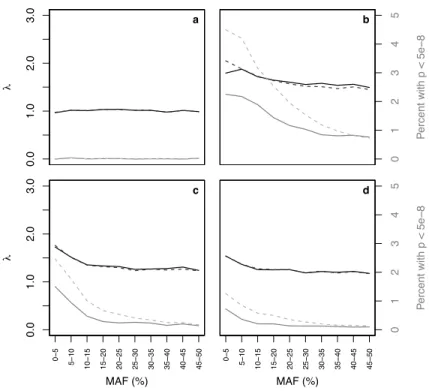
Figure 1.1 summarizes the results of a standard logistic regression analysis, where SNPs are grouped by MAF. For each collection of SNPs, we found the Genomic Controlλ(in black) and the percentage of SNPs
withp <5×10⁻⁸(in gray). Results from the soft call analysis are shown in solid lines, while those from the hard call analysis are shown in dashed lines. In Figure 1.1a, we see thatλ≈1among the 139,732 SNPs measured on both chips, and the percentage of highly significant SNPs is close to 0 across all MAFs; the error measures in this setting are virtually identical whether we use hard call or soft call imputation. Thus,
maf_cat a 0.0 1.0 2.0 3.0 ! maf_cat b 0 1 2 3 4 5 P ercent with p < 5e − 8 MAF (%) c 0 − 5 5 − 10 10 − 15 15 − 20 20 − 25 25 − 30 30 − 35 35 − 40 40 − 45 45 − 50 0.0 1.0 2.0 3.0 ! MAF (%) d 0 − 5 5 − 10 10 − 15 15 − 20 20 − 25 25 − 30 30 − 35 35 − 40 40 − 45 45 − 50 0 1 2 3 4 5 P ercent with p < 5e − 8
Figure 1.1: Black and gray lines represent λvalues and the percentages ofp-values less than 5×10⁻⁸, respectively, for SNPs grouped by minor allele frequency (MAF) in four settings:aSNPs genotyped on both Affy and Illumina platforms;bSNPs genotyped on Illumina platform and imputed for the Affy controls; cSNPs genotyped on Affy platform and imputed for the Illumina controls; anddSNPs imputed for both groups. Solid lines are from soft call analysis and dashed lines are from hard call analysis. Note that in some places (particularly in panela) the solid and dashed lines are indistinguishable because the results from the soft call and hard call analyses were very similar.
when we consider only the SNPs measured on both chips, we have no evidence from these two measures that the distribution of the test statistics deviates from the null.
However, among the 357,361 SNPs measured on Illumina and imputed on Affy (Figure 1.1b), we see an overall increase inλto 1.6. We see an increase in the percentage of highly significant SNPs to1.3% when using soft call genotypes, and to 2.1%when using hard call genotypes. Thus, when using hard call genotypes, 7,644 SNPs are being declared significant at the5×10−8 level. These increases are most prominent among SNPs with low MAF, as shown in the Figure. The Type I error inflation is also apparent, though less dramatic, among the 458,034 SNPs measured on Affy and imputed on Illumina (Figure 1.1c) whereλ = 1.3overall, and where we are seeing0.4%highly significant SNPs when using soft calls and 0.8%highly significant SNPs when using hard calls; we see similar numbers among the 1,392,682 SNPs imputed in both (Figure 1.1d). Results were largely unchanged when we first pooled the two groups and then imputed.
To try to correct these problems, we applied the three described methods. Here, we present results for the SNPs measured on Illumina and imputed on Affy for simplicity; results were similar in the other two problematic cases.
1.3.1 Method 1
We found the first ten PCs using hard call genotypes because those are currently supported by EIGEN-STRAT. We did this once using all SNPs, and once restricting to SNPs measured on Illumina and imputed on Affy. Results were similar in the two approaches, and results from the latter are shown. The top three PCs are plotted against one another in Figure 1.2. We see that the second PC completely separates the cases (i.e., the Affy controls) and controls (the Illumina controls). Thus, when these PCs are included in a logis-tic regression predicting case-control status, we get a complete separation of data points, and the models cannot be fit.
1.3.2 Method 2
We considered restricting to SNPs imputed with increasingly higher quality, as quantified by the imputation R2. Results for the soft call genotypes are shown in Table 1.1. As the R2 threshold was increased, our summary measures improved; however, this happened at the expense of losing SNPs for analysis, which
PC 1
−0.04 0.00 0.03 ! ! ! ! ! ! ! !! ! ! ! ! ! ! !! ! ! ! !!! ! ! ! ! ! ! ! ! !! ! ! ! ! ! !!!! ! ! ! ! ! ! ! ! ! !!! !!! ! ! ! !! ! ! !! ! ! !!!!! !!!! !!! ! ! ! ! ! ! ! ! !!! ! ! ! ! ! ! ! ! ! !!! ! ! ! !!!! ! ! ! ! ! ! !! ! ! ! ! !! !! !! !!! ! ! ! ! ! ! ! !! ! !!! !! ! ! !!! ! ! ! ! !! ! !! !! ! ! ! !! ! ! ! ! ! !!!!!!!! ! ! ! ! ! ! ! ! ! ! ! !!! ! ! !!! ! !!!! ! ! ! ! ! !!!!! ! ! ! ! !! !! ! ! !! ! ! ! ! ! ! ! ! ! ! ! ! ! ! ! ! ! ! ! !!! ! !! !!! !!!!!!! ! ! ! ! ! ! ! ! ! ! ! !!! !! ! !! ! ! ! !! ! ! ! ! ! ! !!! ! !!!!!!!!!!! ! !!! ! ! ! ! ! !!!! ! ! ! ! !! ! ! ! ! ! ! ! !! ! ! ! ! !! ! !!!!!!!! !!! !! ! !!! ! ! ! ! ! ! !! ! ! ! ! ! ! ! !! ! ! ! ! !! ! !!!!! ! ! ! ! ! !!! !!!! !! !! ! ! ! ! ! ! ! !! !!!!!!!!!!!!!!!!! ! ! ! ! !!! ! ! ! ! ! !!! ! !!!! !! ! ! ! ! ! !!!! ! !!! ! ! ! !! ! !! ! ! !! ! !! ! ! ! ! ! ! ! ! ! ! ! !! ! ! ! ! ! ! ! ! !! ! !!!! ! ! ! ! ! ! ! ! ! ! !!!!! ! ! ! !! !! ! ! ! ! ! ! !! ! ! ! ! ! ! ! !! ! ! !!! ! ! !! ! ! ! !! ! !! ! ! ! ! ! ! ! ! ! ! !!! !!!! !!!!!! ! ! ! ! ! ! ! ! ! !!!! ! ! ! ! ! !! ! !!!! ! ! ! ! !! ! !! ! ! ! !!! ! ! ! !! ! ! !! ! !!! ! ! ! !!!! ! ! ! ! ! ! ! !! !!!!!!!!!!!!! ! ! !!!!! !!!!!!! !!! ! ! ! ! ! ! ! !! ! ! !! ! ! ! ! !!!! ! !!! !! ! ! ! ! ! ! !!! ! ! ! ! ! ! ! ! ! ! ! ! ! ! ! ! ! !! ! ! ! ! ! !!! !! !!! ! ! ! ! ! ! ! !! ! ! ! ! ! ! ! ! ! ! ! ! ! !! ! ! !!! ! !! ! ! ! !!!! ! ! !! !!!! ! !! ! ! ! !! ! ! !!! !!! ! ! ! ! ! !!!!!!!! ! ! !!! ! ! ! !!! ! ! ! ! ! ! !! !!! ! ! !! !! ! ! !!! ! ! ! ! !! ! ! ! ! ! ! ! ! !!!!! !! ! !! ! ! ! ! ! !! ! ! ! ! ! !!! !! ! ! ! ! ! ! ! !!!! ! ! ! ! ! ! ! ! ! ! ! ! ! ! ! ! ! !! ! ! !! ! ! ! ! ! ! ! !!!!!!!!! !! ! ! ! !!! ! !!!!! ! ! ! !! ! ! ! ! ! !!!!! ! !! !! ! ! !! !!!!!! !! ! !! !!! ! !!!!! !! ! ! ! ! ! !!!!!! ! ! ! ! ! ! ! ! ! !! !! !! ! !!! ! ! ! ! !!! ! !!!!!!!! ! !! ! ! ! ! ! ! ! ! !! !! ! ! !! ! ! ! ! ! ! ! ! ! ! ! ! ! ! ! ! ! !! !!!! ! !! ! !! ! ! ! !! ! ! !! ! ! ! ! ! !!! ! ! ! ! ! !! !! ! ! !!! !! !! ! !!!!!!! ! !! !! ! ! ! !! ! !! ! ! ! !! ! !! ! ! ! ! ! ! ! ! ! ! !! ! ! ! ! !!! !! ! ! ! !! ! ! !! ! ! !! ! ! ! ! ! ! ! ! ! ! !! ! ! ! ! !! ! ! ! ! ! ! ! !!!! ! ! ! ! !! !! ! ! ! ! ! ! ! ! ! ! !! !! !! ! !!! ! ! ! ! ! !! ! ! !! ! !! ! !!!!! ! ! ! ! ! ! ! ! ! ! ! ! ! ! !! !!!!!! ! !! ! ! ! !! ! ! ! ! ! !! ! ! ! ! ! !! ! !! ! ! ! !!!!! ! ! ! ! ! ! ! ! ! ! ! ! ! ! ! !!! ! ! !!!!!!! ! ! ! ! ! ! ! ! !! ! ! ! ! !! ! !! ! !!!!! !! ! ! ! ! ! !!! ! ! ! ! ! ! ! ! ! ! !! ! ! !!! ! ! ! ! !!! ! !! ! ! ! !! ! !! ! ! ! ! !!!!!!!!!! ! ! !!! ! ! !! !! ! ! ! ! !! ! ! ! ! ! ! ! ! ! !! ! ! ! !!! ! ! ! !!! ! ! ! ! ! ! !! ! ! !! ! ! ! !! ! ! !! ! ! ! ! !!! ! ! ! ! ! ! ! ! ! ! ! ! ! ! ! ! ! ! !!! ! ! ! ! !! !! ! ! ! ! ! !!! ! ! ! ! !! ! !!!!! ! ! !!!!!!!!! ! !!! ! ! ! ! !! ! ! !!! ! !! ! !! ! !! ! ! ! ! ! ! ! ! ! !!! ! !!!! ! ! ! ! ! ! !! ! ! !! ! !! ! !!! ! !! !! !!!! ! ! ! ! !! ! !! ! ! !! !!!!! ! ! !! ! ! ! ! ! !! ! ! ! !!! ! ! ! ! ! ! ! !! ! ! !! ! !! ! ! !! !! ! !! ! ! ! !! !! !! !!!!! ! ! !!!!! ! ! ! ! ! !!! !!! !! ! ! ! !! ! ! !!!! ! ! ! ! ! !! ! ! ! !! ! ! ! ! ! !! !! ! !!!!!!!!!! ! ! !! ! ! ! ! ! ! !! ! !! ! ! ! !! ! ! !! ! !! ! ! !! ! ! !!! ! ! ! ! ! ! ! ! !!! ! ! ! ! !! ! ! ! ! ! ! ! ! ! ! !! !! ! ! !! ! ! !!! ! ! ! ! ! !! ! !!!!!! ! ! ! ! ! ! ! !!! ! ! ! !! ! ! ! ! ! !!! ! ! ! ! ! ! ! ! !! !!! !!! !!!! !! ! !!! ! ! ! ! !!!!! ! ! ! ! ! ! !!!! ! !! ! ! ! !!! !! ! ! ! ! ! ! ! !!! ! ! !!! !! ! ! !! ! ! ! ! ! ! !! ! !! ! ! ! ! !! !! ! ! ! ! ! !! !!! !!! ! ! ! ! ! ! !! ! ! ! ! ! !! !! ! ! !!! ! !! ! ! !!!!!!! ! !! !! !!! !!!!! !! ! ! ! ! ! ! ! ! ! ! ! ! ! ! ! !! ! ! ! ! ! !! !!! ! !! !! ! !! !! ! ! ! ! ! !! ! !!! ! !!!!!!!!! ! ! ! ! ! ! ! ! !!! ! ! ! !!!!!! ! !!! ! !!! ! !! ! ! ! ! ! !! !!!!! ! ! ! ! !!! ! ! ! !! ! ! ! !!! ! ! ! ! ! ! !! ! !! ! ! ! !! ! ! ! !! ! ! ! ! ! ! ! ! ! !! !! ! ! ! ! !!!! ! ! ! !! ! ! ! ! !! ! !!!!! ! !!!!!! ! !!!! ! ! ! !! !!!!! ! !! ! ! ! !!! ! !!!!! ! !! ! ! !!!!! ! ! ! ! !!!!!! ! ! !!!! ! ! ! ! ! ! !! ! ! !!!! !!!!!! ! ! !!! ! ! ! !! !! !! ! ! !!!! ! ! ! ! !! ! ! !! ! ! ! ! ! ! ! ! ! !! !! ! !!! !!! ! !! ! ! ! ! ! ! ! !!! ! ! ! ! ! ! !!!! ! ! ! ! ! ! ! !!! ! ! !! ! ! ! ! ! ! ! ! ! ! ! ! ! ! !!!!!! !!!! ! !!! !! ! ! ! ! !!!!!! ! ! ! ! ! ! ! ! ! !!!!! ! !!!!!! !!!!! ! ! ! ! !! ! ! ! !! !! !!!!!! ! !! ! ! ! ! !!!! ! ! ! ! ! ! ! ! ! ! ! ! !! ! ! ! !! ! ! ! ! !! ! ! ! ! ! ! ! ! ! ! !!! !!!! ! ! ! !!! ! !! ! ! ! ! ! ! ! ! ! ! ! !! ! ! ! ! ! !! ! ! ! !!! ! ! !! ! ! ! ! ! !!!! ! ! ! ! ! ! ! !!!! ! ! ! ! !!!!! !! ! ! ! ! ! ! !! ! ! ! ! ! !! ! ! ! ! !!!! ! ! ! !!!!! ! !! !! ! ! ! ! ! ! ! ! ! !! ! ! ! !! ! !! !!!! ! !! ! ! ! ! ! ! ! ! ! ! ! ! !! ! !!!!! ! ! ! !!! ! ! ! ! ! ! ! ! ! !!!! − 0.10 − 0.02 ! ! ! ! ! ! ! ! ! ! !!!!!!! ! ! ! !!! ! ! ! ! ! ! ! ! ! !!! ! ! ! ! ! ! ! ! ! ! ! ! ! ! ! !!!!!!! ! ! !! !!!!! ! ! !!! ! !!!!! ! !! ! ! ! ! ! ! ! ! ! ! ! ! ! !! ! ! ! !!!!!! ! !! ! ! ! ! ! ! ! ! !! ! ! ! ! ! ! ! ! ! ! !!!!!!! ! ! ! ! !! !!!! !!! ! ! ! ! ! ! ! !! ! !!!!! !! ! ! ! ! ! ! ! !! ! !! !! !! ! ! ! !!!! ! ! ! ! ! ! ! ! !!!!!! ! ! ! ! ! ! !!! ! ! ! ! ! ! ! ! ! ! !!! ! ! !! ! !! ! ! ! ! ! ! ! !! !! ! ! ! ! ! ! !!!!! ! !! ! ! ! ! ! ! ! ! ! ! ! ! ! ! ! ! ! !! ! !! ! ! ! ! ! ! ! ! ! ! ! !! ! ! ! ! ! ! !! ! ! !! !!!! ! ! !!! ! ! !! ! ! ! !!!!!! ! ! ! ! ! ! ! !! ! ! ! ! ! ! !! ! ! ! ! ! !! ! ! !! ! !! !!!! ! ! ! ! ! ! ! ! ! ! !! ! ! ! !! !! ! !! ! ! ! ! ! ! ! ! ! ! ! ! !!!!!! ! ! ! ! ! ! ! ! ! ! ! !!!!!!!!! ! !! !!!!! !! ! ! ! ! ! !! ! ! ! !! ! ! ! !! ! ! ! ! ! ! ! ! ! ! ! ! !! ! !!! ! ! !!!!!! ! ! ! ! !! ! ! ! ! ! ! ! !! ! ! !! ! ! ! ! ! ! !!!! ! ! ! ! !!! ! ! ! ! ! ! ! ! ! ! ! ! !! ! ! !!!! ! ! !!! ! ! ! ! ! ! ! ! ! ! ! ! ! ! ! ! !!! !!!! ! ! ! ! ! !!! ! ! ! ! ! ! ! ! ! !! ! !! !! ! !! ! ! ! ! ! ! ! ! ! ! ! ! !!!! !!!! ! ! ! !! !!! ! !!! !! ! ! ! ! ! ! ! ! !!!!! ! ! ! ! ! ! !! ! ! !!!!! ! ! !! ! ! ! !! !!! !!!! ! ! ! !! ! ! ! ! ! !!! ! ! ! ! !! !!! ! ! !! ! ! ! ! ! ! ! ! ! !! ! !! ! ! !!! ! !!!! ! ! ! ! ! ! ! ! !! ! ! ! ! !! ! ! !! ! ! ! ! ! ! ! ! ! !! ! ! ! ! ! ! ! ! ! ! !! ! ! ! ! ! !!! ! ! !! ! !! !! ! ! ! ! ! ! ! ! !!! ! !!! ! ! ! ! !!!!! !! !! ! !!!!! !! !!!! !! ! !! ! ! ! ! ! ! !! ! ! ! ! ! ! ! !!! ! !! ! ! ! ! ! ! ! ! ! ! !! !! ! ! ! !! ! ! !!!!! ! ! ! !! ! ! ! ! ! ! !!! ! ! !!! ! ! ! ! ! ! ! ! ! !! ! ! !! ! ! ! ! ! ! ! ! ! ! ! !! ! ! ! ! ! ! ! ! ! ! !! ! ! ! ! ! ! ! ! ! ! ! ! !!! ! ! ! ! ! ! ! ! !! ! ! !! !! ! ! ! !! ! !! !! !!!!!!! ! ! ! ! ! !! !!!! !! ! !!!! ! ! ! ! ! !!! !! ! !!! !! ! ! ! !!!!!! ! ! ! ! ! ! ! !!!! ! ! ! ! ! ! ! ! ! ! !! ! ! ! ! ! ! ! ! ! ! ! ! ! ! !!! ! ! ! ! ! ! ! ! ! ! ! ! ! ! ! ! ! ! ! !! !! ! ! ! ! ! ! ! ! ! ! ! ! ! ! ! ! ! ! ! ! ! ! ! ! ! !!! ! ! ! ! ! !! !! ! ! ! ! ! ! ! !! !!!! ! ! ! !! ! ! ! ! ! ! !!! !!!!!!!! ! ! ! ! !!! ! ! ! ! !! ! ! ! ! ! ! !! ! !! ! ! ! ! ! !! ! ! ! ! ! ! ! !! !!!! ! ! ! ! ! !!! !!!! ! ! ! ! ! ! ! ! ! !!! ! ! ! ! ! ! ! !! ! ! ! ! ! ! ! !! ! ! ! ! !!! ! ! ! ! ! ! ! ! ! !!!! !! ! ! ! ! ! ! ! ! ! ! ! ! !! ! ! ! ! !! ! ! ! ! ! ! ! ! ! ! ! ! ! ! ! ! ! ! !!!!!! ! ! !! !! ! ! ! ! ! ! ! ! ! ! !! !! ! ! ! ! ! ! ! ! ! ! ! ! ! ! ! ! !!!! ! ! ! ! ! ! ! ! ! ! ! ! ! ! ! ! !!!!! ! ! ! ! ! ! ! ! ! ! ! ! ! ! ! ! ! ! ! ! !!! ! ! ! !!! ! !! ! !! ! ! ! ! ! ! ! ! ! !! ! ! ! !! ! ! !! ! ! ! ! ! ! ! !! !!! ! !! ! ! ! ! ! !!! !! !! ! ! ! !!! !! ! ! ! ! !! ! ! ! ! ! ! ! !! ! ! ! ! ! ! ! !! ! ! ! ! ! ! !!! !! !! ! ! ! ! ! ! ! ! !! ! ! ! ! !! ! ! ! ! !! ! ! ! ! ! ! ! ! ! !! ! ! !! ! ! ! ! !! ! ! ! ! !! ! ! !!!! !! ! ! ! ! ! ! ! ! ! ! ! ! !!! ! !!!! ! !!!! ! ! !!!! ! ! ! !!!! ! ! ! ! ! ! ! ! ! ! ! ! ! ! ! ! ! ! ! ! ! ! !! !!! !! ! !!! ! ! ! !! ! ! ! ! !!!! ! ! ! ! ! ! ! ! ! !!!!! !! ! ! ! ! ! ! ! !!! ! !! !!!!! ! ! ! ! ! ! ! ! ! !! ! ! ! ! !!! ! ! ! ! !! ! ! ! ! ! ! !! ! ! ! ! ! ! ! ! ! ! ! ! !! ! ! !!! ! ! ! ! ! ! ! ! ! ! ! ! ! ! !!!!!!!!!! ! ! ! ! ! ! ! ! ! ! ! ! ! ! ! !!! ! ! ! ! ! ! ! ! ! ! ! ! ! !! !!!! ! ! !! !!! ! ! ! ! ! ! ! ! ! ! ! ! ! ! !! ! ! ! ! !! ! ! ! ! ! ! ! ! ! ! ! !!! ! ! ! ! ! ! ! ! ! ! ! ! ! !! ! ! ! !! ! !!! ! ! ! !! ! ! !! ! ! ! ! ! ! ! ! ! ! ! ! !! ! ! ! !!! !!! ! ! ! ! !! ! ! ! ! ! ! ! ! !!! ! ! ! ! ! ! ! ! ! ! ! !!! ! ! !!! ! !! !!! ! ! !! ! ! ! ! ! ! !! ! !!! ! ! ! ! ! !!! ! ! !! ! ! !!! ! ! ! ! !! ! ! ! ! ! ! ! !! !! ! ! ! ! !! ! ! ! ! !! !! ! !! ! ! ! ! ! ! ! ! !! ! ! ! ! ! !! !!!! ! ! ! ! ! ! !! ! ! ! ! !! ! ! ! ! ! ! ! ! !!! ! ! ! ! ! ! ! ! ! ! ! ! ! ! ! ! !!! ! ! !! ! ! ! ! !! ! ! ! ! ! ! ! ! ! !! !! ! ! ! ! !! ! !! ! !!!! !!!! ! ! ! ! !! ! ! ! ! !! ! ! !!!! ! ! ! ! ! ! ! ! ! ! ! ! ! ! ! ! ! ! ! ! ! ! ! ! ! ! !! ! ! !! ! ! ! ! ! ! ! ! !! ! ! ! !! ! ! ! ! !! ! ! ! ! ! ! ! ! !!!! !! ! ! ! ! ! ! ! ! ! ! ! !! ! ! !! ! ! ! ! ! ! ! ! !! ! ! ! ! ! ! ! ! ! !!! ! ! ! ! ! ! ! ! ! ! !! ! !! !!! ! ! ! ! !!!!! ! ! ! ! ! ! ! ! ! ! ! ! !! ! ! ! ! !! !!!!!!! ! ! !! ! ! ! ! ! ! ! ! ! !!! ! !! !!! !! ! ! ! ! ! ! !! ! !! ! ! ! !!!!!!! ! ! ! ! ! ! ! ! ! !! ! ! ! ! ! ! ! !!! ! !! ! ! ! ! ! ! !!! ! !!! ! ! ! ! ! !!! ! !! ! !!! ! ! !! ! !! ! !! ! ! ! ! ! ! ! ! ! ! ! !! ! ! !! ! !! ! !! ! ! ! ! ! !! !! ! ! ! ! ! ! ! ! ! ! ! ! ! ! ! !! ! ! ! !! ! ! ! ! ! ! ! !!! !! ! !! ! ! ! ! ! !! ! !!!!!!! ! !!!!! ! ! ! ! ! ! ! ! !!! ! ! ! !! ! !! !! ! !! ! ! ! ! ! ! ! ! !! ! ! !! ! ! ! ! !! ! !! ! !! ! !!! ! ! ! ! ! ! !!! ! ! ! ! ! ! !!!! !!!! !! ! ! ! ! ! ! ! ! ! !! ! ! ! ! ! ! !! ! ! ! !! ! ! ! ! !!! ! ! !! !! ! ! ! ! !!! ! ! ! !!! ! !!!! ! ! !!! ! ! !! ! ! ! !!! ! ! ! ! ! ! ! ! ! !! ! ! ! ! !!!! ! ! ! ! !!! ! ! !!!! ! ! ! !! ! ! ! !!! ! ! ! !!!!!! ! !! ! !!! ! ! ! ! ! ! ! ! ! ! ! !! ! ! ! !!! ! ! ! !!! ! ! ! ! ! ! ! ! ! ! ! ! ! − 0.04 0.00 0.03 ! !! ! ! ! ! !!! ! ! !! !!! ! ! !!!! ! ! ! ! ! ! !! !!!! ! ! !!!!! ! ! ! ! ! !!!!!!!!!! ! ! ! ! !!! ! !! ! ! ! !!! !!!!!!! ! ! !! ! ! !!!!!! !! ! ! ! !!! !!!! ! ! !! ! ! ! ! ! ! !!! !!! ! ! ! ! ! ! !!! !!!!!! ! ! ! ! ! ! !! ! ! !! ! !! ! ! !!! !!!!!!! !!!!!!! ! ! ! ! ! !!!!!! ! ! !! !! ! ! ! ! ! ! ! ! !! !!! ! ! !! ! ! ! ! !!! !!! ! !! !! ! !!! ! !!! ! ! ! ! ! ! ! ! ! ! !! !!! ! ! ! ! !!!! ! ! !! ! !!! !! ! ! ! ! ! ! ! !! ! ! ! ! ! !!!! ! !! ! ! ! ! ! ! ! ! !! ! !! ! !! !!! !!!!!! ! ! ! ! ! ! ! ! ! ! ! !!!!!!!!! ! ! ! ! ! ! ! ! ! ! ! ! ! !!! !!! ! ! !! !!!! ! !!!!!!!!!!! ! ! ! !!!! !! !! ! !! ! ! ! ! ! ! !!! !!!! !! ! !!! !!!! ! ! ! ! ! ! !!!!!!!!! ! ! ! !!!! !!!!!! ! ! ! !!!!! ! ! ! ! !!!!!!! ! !!! ! ! ! !!!!! ! !!! ! !! ! ! ! ! ! ! ! !!!! ! ! !!!!!! ! ! ! ! !!!! ! !!!! !!! ! !!!!!!!! ! !!! ! ! !!! !! ! ! !!!!!! ! ! ! ! ! ! ! ! !! !!!!!! ! ! !!!!!!!!! ! !! ! !! ! ! ! ! !! ! ! ! ! !! !!! !! !!! ! ! ! ! !! !! ! ! ! ! !! !!!! !!! !! !! ! !! ! !!!!!! ! !! ! !! ! ! !!!!! ! ! !! ! ! ! ! !!! ! ! !! ! ! !! ! ! ! ! !!!!!!!!!!!!!!! ! !! ! !! ! ! ! ! !! ! ! !! !! ! ! ! ! ! ! ! ! ! ! ! ! !! ! !!!! !!!!!!!!!!!!!!! ! ! !! ! !! ! !!! ! ! ! ! ! !!!!! ! ! !!!! !!! ! ! ! ! !! ! ! ! ! ! ! !!!!!!! ! ! ! !!!! ! !!!! ! ! ! !!! ! ! !! ! !!!!!!! ! !!! ! !!!!!!!!!!! ! ! ! ! !!! !! !!!! !!!!! ! ! ! ! ! ! ! ! ! ! ! ! !!!!! ! !!!!! ! !!!! ! ! ! ! ! ! ! ! !! ! ! !!!!!!! ! ! ! ! ! ! !!! !!!! !!! ! !! !!! !!! ! ! ! ! !! !!!! !!! !!! ! !!! ! ! ! ! ! ! ! ! ! !! ! !!! ! !! !!!! ! ! !!! ! !!!!!!! ! ! ! ! ! !!!!!!! ! !!!!!!!!!!!!!! ! !!!!! !!!!!!!!!!! ! ! !!!! !! !! ! ! ! !!! !! ! ! ! ! ! ! ! ! ! ! !! ! ! !!!!!! ! !! ! ! ! ! !! ! ! !!!!! ! ! !!! ! !! ! !! !!!! ! ! !! ! ! ! ! ! ! !! ! ! ! ! ! ! ! ! ! ! ! ! !!! ! ! ! ! !! ! ! !!! ! ! ! ! ! ! ! ! ! ! ! !! ! ! ! !!!! ! ! ! ! !! ! ! ! ! ! !!!!! ! ! ! !! !! ! ! !! !! !! ! ! ! ! !!! ! ! ! ! ! ! ! !! ! ! !!!! ! ! !! ! !! ! !!!! ! ! ! ! ! ! ! !! ! ! ! ! ! ! ! ! !!! ! ! ! ! ! ! ! ! !! ! ! ! ! !!! ! ! ! ! !!! ! !!!!!!!!!!!!!!!! ! ! ! ! ! ! ! ! ! !! ! ! !!! ! ! ! ! !!! ! ! ! ! ! ! ! !! ! ! !!!!! !!!!!!! !!! !! ! !! ! ! ! ! !!! ! ! ! !!!!!!! ! ! ! ! !!! ! ! ! ! ! ! ! ! ! ! ! !! ! ! ! !! ! ! ! ! ! !!!! ! ! ! ! !! ! ! ! !! ! !! ! !! ! ! ! ! ! ! ! ! ! ! ! !!!!! !! !!! ! ! ! !!! !!! ! ! ! !!!!!! ! ! ! ! ! !!!! ! !! ! !!! ! ! !!! !!!!!!!!! ! !!! ! ! ! ! ! ! ! ! ! ! ! ! ! ! ! ! !!!! !! ! ! ! ! ! !! ! ! ! !!! ! ! ! ! ! ! ! ! ! ! !! ! !! ! ! ! ! !! !! ! !! !! ! ! !! ! ! ! ! ! ! ! !!!! ! ! ! ! !! ! ! !!! ! !!! ! ! ! ! ! ! ! !!!!!!! ! !!!! ! ! ! !! !! ! ! ! ! ! !!!! ! ! ! ! ! ! ! ! ! ! ! ! ! ! ! ! ! !! ! ! !! ! ! ! !! ! ! ! ! ! ! !! ! ! !!! ! ! ! ! ! ! ! ! !!!!!! ! !!!! ! ! !! ! ! !!!! !! ! !!!!!!!!! ! ! ! ! ! ! !! ! ! !! ! ! ! !!! !!! ! ! !! ! ! ! !!!!! ! !!! ! ! ! ! !!! !!!!!!!! !!!! ! ! ! !! ! ! ! ! !!! ! !!!! ! ! ! ! ! !! !! ! !!! !!!!!!!! ! ! ! !! ! ! !!! ! ! !! !!!!!!!!!!! ! !! ! ! ! ! !! ! ! !!!! ! ! ! !! ! ! !! ! !! ! ! !! !!!!! ! !! ! ! ! ! !!!! !! !! !! ! ! ! ! ! ! !! ! ! ! ! !!! ! ! ! !!!!!!!! ! ! !! ! !!!! ! !!! ! ! !!!!!!! !!!! ! !! !!!!! ! ! !! !! !! ! ! !!! !!! !! ! ! ! !! ! ! ! ! !! ! !!! ! ! !!! ! !!! ! !!! !!! !!!!! ! ! ! ! ! ! ! ! !! ! !!! ! !!!! ! ! ! ! ! ! ! ! ! ! ! ! ! !! ! ! ! ! ! ! ! ! !! ! ! ! ! ! !!!!!! ! ! ! ! ! ! !! ! !! !!!!!!! ! ! ! ! !!!! ! !! ! ! ! !! ! ! ! !! !!!!!!!! !! ! ! !!!! ! ! ! ! ! ! ! !!!! ! ! ! ! ! !!!!!!!! !!! ! !!! ! ! !! !!! !!!!! ! !!!! ! ! !! ! ! !!! !! ! ! ! ! ! ! ! ! ! ! !!!! !!!! ! !! ! !!!! ! !!!!!!!!! ! ! ! !! ! ! ! ! ! ! ! !!! ! !! ! ! ! ! !! !!!!! ! ! !!!!!!!! !!!!! ! ! ! ! ! ! !! ! !! ! ! !!! ! ! ! !! ! ! ! !!!!!!!!!!!!!!!! ! ! ! !! !! ! ! ! !!!! ! ! !! !!! !!!!!!!! !!!!! ! ! !!! ! ! ! ! ! ! !! ! !! ! !! ! !! ! ! ! !!!!!!!!!!!!!!!! ! ! ! ! !! ! ! !!! !!! ! !!! !!! !!! ! ! ! ! ! !!! ! ! !!!!!! !!!! ! ! !!!! ! ! ! ! ! ! !!!! !!!! ! ! ! !! ! ! ! ! ! !!!! ! ! !!! ! ! !!! ! ! ! !! ! ! !! ! ! ! ! ! !!! !! !!!!!!!!! !! ! ! ! !!!! ! !! ! ! ! ! ! !! ! ! !!!!! ! ! ! ! ! !!!! ! ! ! ! !! ! !!!!!!!!!!! !!!!!!!!!!!!!!! ! ! !! !! ! !!!! ! ! ! ! !! !!!! !! !!! ! !!! ! ! !! !!! ! !!! ! ! ! !!! !!!! ! ! ! ! ! !! ! ! ! ! !!! ! !!! !! ! ! ! !! ! ! ! !!! ! ! ! ! !! !! ! ! !!! !! !!! ! ! ! ! !!!!!!!!!!! ! ! ! !! ! ! ! ! ! !! ! !! ! ! ! !!!!! ! ! !! ! ! ! ! ! ! ! ! !! ! ! ! ! ! ! ! ! ! !!! ! !! ! ! ! ! !!! ! !!!! !! ! ! ! ! !! ! ! !! !! !! !! !!!!!!! ! !!! ! !! ! !PC 2
!! ! ! ! ! ! ! ! ! ! !!!!! !! ! ! !!! ! !! ! ! ! ! ! !! !!!!!! !!!!! ! ! ! !!!!!!!!!! ! ! ! !!!!!! ! ! !!! !!!!! ! ! ! ! ! !!!!!!!! !!! ! ! ! ! ! ! !!!!! ! ! ! ! ! ! ! ! ! ! ! ! !! ! ! ! ! !! ! ! ! ! !!!!!!!! ! ! ! !!!!!!!!!! ! ! ! ! ! ! !! ! !!!!! !!!!!!!! ! ! ! ! !! !! !!!! ! !!!! ! ! ! ! ! ! ! ! !!!!! ! ! ! ! ! ! ! !!!!!! ! ! ! ! ! ! !!! ! ! ! ! ! ! ! ! ! ! ! ! !!!!! !! ! ! ! ! ! ! ! !!!! ! ! ! ! ! ! ! ! !! ! ! ! ! ! ! ! ! ! ! !! ! !! ! ! ! ! ! ! ! ! !! ! !! ! ! ! ! ! ! !! ! ! !! !!!!! ! ! ! ! ! !!! !!! ! !!!!! ! ! ! ! ! ! !!! ! ! ! ! ! ! !! ! ! ! ! !!! ! ! ! !!! !!!!!!!!! ! ! ! ! !!!!!! !! ! ! ! ! !! ! ! ! ! !!!!!!!!!!!!!!! ! ! ! ! ! ! ! ! ! ! !!!!!!!!! ! !!!! !! ! !!! ! ! ! ! !! ! ! ! !! !! ! ! ! !!! ! ! ! ! ! ! !!! !!! !!! ! ! !!!!!! ! ! ! ! ! ! !!! ! !! ! !! ! ! ! ! ! ! !!!!!!!! ! ! !!!! ! !!!!!!!! ! ! ! ! !!! !! !!!!!!! !! ! ! !!!!! ! ! !! ! ! ! ! !! ! !!!!! ! ! ! ! !!! ! ! ! !! !! ! ! !! ! !! !! ! !!! !! ! ! !!! ! !! ! ! ! !! !! !!! !! ! !!! !!!!! ! !!!!!! ! ! !!!!! !! ! ! ! ! ! ! ! !! !! ! ! ! ! ! ! ! ! ! ! ! ! ! ! ! !!!! ! !!!!!!! ! ! !!!! !!!!!!! ! ! !!! ! ! ! ! !!! ! ! ! !! !! !!!!!!!!!!!!! ! ! ! ! ! !!! !!!!!! ! !! ! !! ! ! ! !! !!!!!!!!! ! ! ! ! ! ! ! ! ! ! ! !!!!!! !! !!! ! ! ! ! !!! ! ! !!! ! ! ! ! !! ! ! !! ! !! ! ! !! ! !!! ! ! ! ! !!!! ! ! ! !!!! ! ! ! ! ! ! ! ! ! ! ! !!! !! ! !! ! ! ! ! ! ! ! ! ! ! !! !!!!! ! ! ! ! !!!! ! ! ! ! !!! ! ! ! ! ! !! ! ! ! !! ! ! ! ! ! ! ! ! ! ! !!!! !! ! ! ! ! ! ! !!! ! !!! ! ! ! ! ! !!! ! !!! ! ! ! ! !! ! ! ! ! !!!!! ! ! ! ! !! ! ! !! ! ! !! ! !!!!!!!! ! !! ! ! !! !!! ! !! ! ! ! !!!! ! ! ! ! !!!!!! !!!!!!!!!!!! !!! ! ! !!!!!!! ! ! ! ! ! ! !!! ! ! ! ! ! ! !!!!!! ! !! ! !! !! ! !!!!!! !!! ! !!!!! ! ! ! ! ! ! ! !!!!!! ! ! ! ! ! !! !! ! !!! !! ! ! ! ! ! ! ! !! ! ! ! ! !!!!!! ! ! !!! ! ! !! ! ! ! ! ! ! ! ! !!!!!!!!! ! ! !!! !!!! !!! !!!!! ! ! ! !!!!!!!!! ! ! ! ! ! ! !!!!!!!!! !!!! ! ! ! ! ! ! !! !!!! ! !!! ! !!! !!!! ! !! ! ! !! ! !!!! ! ! ! ! ! !!! ! ! ! ! ! ! ! ! !! ! ! ! ! !!!!!!!!!! !!!!!!!!! ! ! ! ! !!! !! ! ! ! ! ! ! ! !! ! ! ! ! ! ! ! ! ! ! ! ! ! ! ! ! ! ! ! !!!!!! ! !!!!!!!! ! ! ! ! ! ! ! !! ! ! ! !!!! !! !!!! ! ! ! !! ! !!! ! !! !! ! ! ! ! !! !!!! ! ! ! !!! ! ! !!! !! ! ! ! ! ! ! ! ! ! ! ! ! ! !! ! ! ! ! !! ! ! !! ! !! ! !! !! !! ! ! !! !!!! ! ! !! ! !! ! ! ! ! ! !! ! !!!!! ! !!! ! !!! !! ! ! ! !!!!!! ! ! ! ! !!!!! ! ! ! ! ! !! ! ! ! !!!!!!!!!!!!!! ! ! ! !! ! ! ! ! ! !!!! ! ! ! ! ! !! ! !! ! !!!! !! ! ! ! ! ! ! !! ! ! ! ! ! !! ! ! ! ! ! ! !!!!! !!! !! ! ! ! ! ! ! ! !!!!!!! ! ! !!!! ! ! ! !!! ! !!! !!!!!!! ! ! ! ! !!!! ! ! !! ! ! ! ! ! ! ! ! ! ! ! ! !!! ! !!! !!! ! ! ! ! !! !! ! !!! !!!! !! !! ! ! ! !! !! ! ! ! !!! !!!!!!!!!!!!! !! ! ! !! ! ! ! ! !! !!!!!!!!!! ! ! ! ! ! ! ! ! ! !! ! ! ! ! ! ! ! ! ! ! ! ! ! !!!!! ! ! !! ! !! ! ! ! ! ! ! ! ! !!! ! ! ! ! ! ! ! ! ! ! ! ! !!!!!! ! ! !!!!! ! ! ! ! ! ! !!!!! ! ! !!!!!!!! !!!! !!!!! !! !! ! ! ! ! ! ! ! !! ! !! !!! ! ! ! ! ! ! ! !!! !!!! !!!!!!!!!! ! ! ! ! ! !!! ! ! ! !! ! ! ! ! ! ! ! ! ! ! ! ! ! !!! !!!! ! !!! ! ! !!!!!! ! ! ! ! !! ! !!!!! !!!! ! ! ! ! ! ! ! ! ! ! ! !!! !!! ! !! ! !! !! ! !! ! !!!!!! !! !! !!!!!!!!!!!!!!!!!! !! ! ! ! ! ! ! ! ! ! ! ! !!!!!!! ! !! !! ! !!! ! ! ! ! ! !!! ! ! ! ! !!! ! ! ! ! ! ! ! !! ! !! ! ! ! ! ! ! ! ! ! ! ! !!!!!! ! ! ! ! !!!!!!! !! !! ! !!! ! ! ! !!! ! ! ! ! ! ! ! ! ! ! !!!! ! ! ! ! ! ! ! ! ! ! !! !! ! ! !! !!!!!!!!!!! ! !! !!! ! ! ! ! ! ! ! ! ! !!!! ! ! ! !! !!!! !! ! !! ! !!! ! ! ! ! ! ! ! ! !! ! ! !! ! ! ! !!!!!!! ! ! ! !!!! ! ! !! ! ! !! ! !!!!!! !! ! ! !!! ! !!!! !!!!!!!! ! !! ! ! !!!!!! ! ! !!!!! ! !!! !!!!! ! ! ! ! ! !! ! !! ! !! !!!!!! ! ! ! ! ! !!! ! ! !!! ! ! ! !! ! !!! ! !!!!!!! ! !! ! ! ! ! ! !! ! !! ! !! ! !! !!! !! ! !! ! ! ! !! !! ! ! ! ! !! !! !! ! ! !! ! ! ! !! ! !! ! !!!! ! ! !!! !!! ! ! !!! ! !!! !! ! ! ! ! ! !!!!! ! !! ! !! ! ! ! ! ! ! !!!!!!!!!!!!! ! ! ! !!! ! !!!! ! ! !! ! !!! ! ! ! ! ! ! ! ! ! !! ! ! ! ! ! ! !! ! !!!! ! ! ! ! ! !!!! ! !!!!! !!!!!! ! ! ! ! ! !!!! ! ! ! ! !!!!! ! ! !!! !! ! ! ! ! !! ! !! ! !!!!!!! ! !!!!!!! ! ! !! ! ! ! ! ! ! !!!!! ! !! ! ! !! ! ! !! !!!! !!!!!!!!!!!!! ! ! ! ! !!!!! ! ! ! ! ! ! ! ! ! !! !! !!!!!!!! !! !! ! ! ! !!! !! ! ! ! !! !!! ! !!!! !!!! ! ! !!! ! ! !! !!! !! ! !!! ! ! ! ! !! !! !! ! ! !!!!!!!!!!!!!!!!! ! ! !! ! ! !! !! !!!!! ! ! ! ! ! !! ! ! !!! !!!!!!!! ! ! ! ! ! ! ! ! !!!! ! ! !!!!! ! ! ! ! ! ! ! !! ! ! −0.10 −0.02 ! ! ! ! ! ! ! !!! ! ! !! !!! ! !! !!!! ! ! ! ! ! ! ! !!!! ! ! ! ! ! ! ! ! ! ! ! ! ! !! ! !! !!! ! ! ! ! ! ! ! ! ! ! ! ! ! ! ! ! ! ! !! ! ! ! ! ! ! !! ! ! !! ! ! ! ! ! ! ! ! ! !! ! !! ! ! ! !! ! ! ! ! ! ! ! ! ! ! ! ! ! ! ! ! ! ! ! ! ! ! ! ! ! ! !! ! !! ! ! ! ! ! ! ! ! ! ! ! ! ! ! ! ! ! ! ! ! ! !! ! !! ! !! !! ! ! ! ! ! !!!!!! ! ! ! ! ! ! ! ! ! ! ! !!! !! ! ! ! ! ! ! ! ! ! ! ! !!! !! ! ! ! ! !! ! ! ! !! ! !! ! ! !! !! ! ! !! !!!!! ! ! ! ! ! !!! ! ! !! ! ! ! ! !! ! ! ! !! ! ! ! ! ! !!!!!!!! ! ! ! ! ! ! ! ! ! ! ! !!! ! ! ! ! ! !!! ! ! ! ! ! ! ! ! ! ! ! ! ! ! !! ! ! ! ! ! ! ! ! ! ! ! ! ! ! ! ! ! ! ! ! ! ! ! !!! ! ! ! ! ! !! ! ! ! ! ! ! ! ! ! ! ! ! ! ! ! ! ! ! ! ! ! ! ! ! ! ! ! ! ! ! ! ! ! ! ! ! ! ! ! ! ! !! ! ! ! !! ! !! ! ! ! ! !! ! ! ! ! ! ! ! ! ! ! ! ! ! ! ! ! ! ! ! ! ! ! ! ! ! ! ! ! ! ! ! ! ! ! ! ! ! ! ! ! ! ! !! !! ! ! ! ! ! !! ! ! ! ! ! ! ! !!! !!!! !!! ! ! ! ! ! !! ! ! !!! ! ! ! ! !! ! ! ! ! !! ! !! ! ! ! ! !! ! ! ! ! !! ! ! ! ! ! ! !! ! ! ! ! !! ! ! ! ! !! ! ! ! !!! ! ! ! ! ! ! ! ! ! ! !! !! ! ! ! ! ! ! ! !!! ! ! ! ! ! ! ! ! ! !! ! !! !! ! ! ! ! ! ! ! ! ! ! ! ! ! ! ! ! ! !! ! ! ! ! ! ! ! ! ! ! ! ! ! ! !! ! ! ! ! ! ! ! ! ! ! ! !!!! ! ! ! ! ! ! ! ! ! ! ! ! ! ! ! ! !! ! ! ! !! ! ! ! ! ! ! !!! ! ! !! ! !! ! ! ! ! ! ! ! ! ! ! !! ! ! ! ! !! ! ! ! !!!!! ! ! ! ! ! ! ! ! ! !! ! !! ! !!! ! ! !! !!! ! ! ! ! ! !! ! ! !! ! ! ! ! ! ! ! ! ! !! ! ! ! !!! ! ! ! ! !! ! ! ! ! ! ! ! ! ! ! ! ! ! ! ! ! ! ! ! ! ! ! ! ! ! ! ! ! !! !! ! ! ! ! !! ! !!! ! ! ! ! ! !! ! ! ! ! !!! ! ! ! ! ! ! ! ! ! ! !! ! ! ! !! ! ! !!!!! ! !! ! ! ! ! ! ! ! ! ! ! !! ! ! ! ! ! ! ! ! ! ! ! ! !! ! ! !! !!!!! ! ! !! ! ! ! ! ! ! ! ! ! ! ! ! !! ! !!! !!! ! ! ! !!! !!! ! ! ! ! ! !! ! ! ! ! ! ! !!! ! !!! ! ! ! ! ! ! ! ! ! !! ! !!!!! ! ! ! ! ! ! ! ! ! ! ! ! ! ! ! ! !! ! ! ! ! ! !!!! ! ! ! ! ! ! ! ! !!!!! ! ! !!! ! ! ! ! ! ! ! ! ! ! ! !! ! ! ! ! ! ! ! !! ! !! ! ! ! ! ! ! ! ! !! ! ! ! ! ! ! ! ! !!! ! ! ! ! ! ! ! ! ! ! ! ! ! ! ! ! !! ! ! ! ! !! ! ! ! !! ! ! ! ! ! !! ! ! ! ! ! ! ! ! ! ! ! ! ! ! ! ! ! ! ! ! ! ! ! ! ! ! ! ! ! ! ! ! ! !! ! ! ! ! ! ! ! ! ! ! ! ! ! ! ! ! ! ! !! ! ! ! ! !! ! ! ! ! ! !! ! !!! ! !!!! ! ! ! ! ! ! ! ! ! !! !!! ! ! ! ! ! ! !! ! !! ! !!!!!!! ! ! ! ! ! ! ! ! ! ! !! ! ! ! ! ! ! !! ! ! ! ! !! ! ! ! ! ! ! ! !!!! ! ! ! ! ! ! !! ! ! ! ! ! ! ! ! ! ! ! ! ! ! ! ! ! ! ! ! !! ! ! ! !! ! ! ! ! ! ! ! ! ! ! ! ! ! ! ! !! ! ! !! ! ! ! ! ! ! ! !! ! ! ! ! ! ! ! ! ! ! ! ! ! ! ! ! ! ! ! ! !! !! !!! ! ! ! ! ! ! ! ! ! ! ! ! ! !! ! ! ! ! ! ! ! ! ! ! ! ! !! ! ! ! ! ! ! ! ! ! ! ! ! !!! ! ! ! !!!!! ! ! ! ! ! ! ! ! ! ! ! !! ! ! ! ! ! ! !!! ! ! ! ! ! ! ! ! !! ! !! !! !! ! ! ! ! ! ! ! ! ! ! ! ! ! ! ! ! ! ! ! ! ! ! ! ! ! ! !! ! !! ! !! ! ! !!!!!!! ! ! !!!! !! ! ! ! ! ! ! !! ! ! ! ! ! ! ! ! ! ! !!!! !! ! !! ! !!! ! ! !!!! ! ! ! ! ! ! ! ! ! ! ! ! ! ! ! ! ! ! ! ! ! ! ! ! ! ! ! ! ! ! !! ! !!!! ! ! !!! ! ! ! ! ! !! ! ! !!! ! !! ! ! ! ! ! ! ! ! ! ! ! ! ! ! ! ! !!!! ! ! ! !! ! ! ! ! ! ! ! ! ! ! !! ! !!! ! ! ! ! ! ! ! ! ! ! ! ! !!! ! ! ! ! ! ! !!! ! ! ! ! ! ! ! ! ! !!!!! ! ! ! ! ! ! ! ! ! ! ! ! ! ! ! ! ! ! ! ! ! ! ! ! ! ! ! ! ! ! ! ! !!!! ! !! ! ! ! ! ! ! ! ! ! ! ! ! ! ! ! ! !! ! ! ! ! ! ! ! ! ! !!!!! ! ! ! ! ! ! ! ! ! ! ! ! !!!!!! ! ! ! ! ! ! ! ! ! ! ! ! ! ! ! ! ! ! ! ! !! !! ! ! ! ! ! ! ! ! ! ! !! ! ! !!! ! !! ! ! ! !! ! ! !!! ! ! !! !!!!!! ! ! ! !! ! ! ! ! ! ! ! !! ! ! !!!!! ! ! ! ! ! ! ! !! !! ! ! ! ! ! ! ! ! ! ! ! ! ! ! ! ! ! !! ! ! ! ! ! ! ! ! ! ! ! ! ! ! ! ! ! ! ! !!! ! ! ! ! ! ! ! ! ! ! ! ! ! !! ! ! !!! ! !!! ! !!!!! !! ! ! ! ! ! ! !! !! ! !! ! ! ! ! ! ! !!!! ! ! ! ! ! ! !! ! ! ! !! ! ! ! ! ! ! !!!! ! !!! ! ! ! ! ! ! ! ! ! ! ! ! ! ! !! ! ! ! ! ! ! ! ! ! ! ! ! ! ! ! ! ! !! ! ! ! ! ! ! ! ! ! ! ! ! ! ! ! ! ! ! ! ! ! ! ! !!! ! ! ! ! ! !! ! ! !! ! ! ! ! ! ! ! ! ! ! ! ! !! ! ! ! ! ! ! ! ! !! ! ! ! ! ! ! ! ! ! ! ! ! ! !! !!!!!! ! ! ! ! ! ! !!! !! ! !! ! ! ! ! !! ! ! ! ! ! ! ! ! !! ! !!! ! !! ! ! ! ! ! ! ! ! ! ! ! ! ! ! ! ! ! !!!!! ! ! ! ! ! ! ! ! ! ! ! ! ! !! ! ! ! !! ! !!! !!! ! ! ! ! ! ! ! ! ! ! ! ! !! ! !! !! ! ! ! ! ! ! ! !! ! ! ! !!! ! !! ! ! ! !! ! ! ! ! !! ! ! !! ! ! ! ! ! ! ! ! ! ! ! ! ! ! ! ! ! !! ! !! ! ! ! !! ! ! ! !!! !! ! !! !!!!!!! ! ! ! ! ! ! ! ! !!! !! ! ! ! ! ! ! ! !! ! ! ! !!! ! ! ! ! !! ! ! ! ! ! ! !! ! ! ! ! ! !!! ! ! ! ! !! ! ! ! ! !! ! ! ! ! ! ! ! ! ! !! ! ! ! ! ! ! ! ! ! ! ! ! ! ! ! ! !!! !! ! ! !!!!! ! ! ! ! ! ! ! ! ! !!! ! ! ! ! ! ! ! ! !! ! ! ! !! ! ! ! ! ! !! ! ! ! ! ! ! ! ! ! ! ! ! ! ! ! ! ! ! ! ! ! ! ! ! ! !! ! ! ! ! !!! ! ! ! ! ! ! ! ! ! ! ! ! ! !!!! ! ! ! ! ! ! ! ! !!! ! ! ! ! ! ! ! ! ! !! ! !! ! ! ! ! ! ! ! !!!! ! ! ! ! ! ! !!!! ! ! ! ! ! !! ! ! ! !! ! ! ! ! ! !! ! ! ! ! ! ! ! ! ! ! ! ! ! ! ! ! !!! ! ! !! ! ! ! ! ! ! !! ! ! ! ! !! ! ! !!!!! ! ! !! ! ! ! ! ! ! ! ! ! ! ! !! ! !! ! ! ! ! ! ! ! ! ! ! ! ! ! ! ! ! ! !! ! ! ! ! ! !!! ! !! ! ! ! ! ! ! ! ! ! ! ! ! ! !! ! !!!!! ! ! !!! ! ! ! ! ! ! ! !! ! ! ! !! ! ! ! ! ! ! ! ! ! ! ! ! ! !! ! ! ! ! ! ! ! ! ! ! ! ! ! ! ! ! ! ! ! ! ! ! ! ! ! ! ! !! ! ! ! ! ! ! ! ! ! ! ! ! ! ! ! ! ! ! ! !! ! ! ! ! ! ! !! ! ! !! !!! ! ! ! ! ! ! ! ! ! !! ! ! !! ! ! ! ! ! !! ! ! ! !!! ! !! ! ! !!! ! ! ! ! ! ! ! ! !!! !! ! ! ! ! ! ! ! ! !!! ! ! ! ! !! ! ! ! ! ! ! ! ! ! ! ! ! ! ! ! !! ! ! ! ! !!! ! ! !! ! ! ! ! ! ! ! !! ! !!!! ! ! ! ! ! !!! ! ! ! ! ! ! !! ! ! !! ! !! ! ! ! !! ! ! ! ! ! !!! ! ! ! ! ! ! ! ! ! ! ! ! ! !! ! ! ! !! !! ! ! ! ! ! ! ! !!!! ! !!!! ! ! ! ! ! ! !!!!!! ! ! ! ! ! !! ! ! ! !!! ! !!!!! ! ! ! !! ! ! ! ! ! !! ! ! ! ! !!! ! ! ! !!!!! ! ! ! !! ! ! !!! ! ! ! ! ! ! ! ! ! ! ! ! ! ! !!! ! ! ! !! !! ! ! ! !!! ! ! ! ! ! !! ! !!! ! ! ! ! ! ! ! !! ! ! ! ! ! ! ! ! ! ! ! ! ! ! ! !! !!! !! ! ! ! ! ! ! ! ! ! ! ! ! ! ! ! ! ! ! ! ! ! !! ! !! ! ! ! !! ! ! ! ! ! ! ! ! ! ! ! ! ! ! ! !! ! ! ! ! ! ! ! ! ! ! ! ! ! ! ! ! ! ! ! ! ! ! ! ! ! ! ! ! ! ! ! ! !! ! !! ! ! ! !! !! ! ! ! ! ! !!! ! !! ! ! ! !!! ! ! ! ! ! ! ! ! ! ! !! ! ! ! ! !! ! ! ! ! ! ! ! ! ! ! !! ! !! ! ! ! ! ! !! !!! ! ! ! !! ! !! ! !!!!! ! ! ! !! ! ! ! ! ! ! !!!!! ! ! !!! ! ! ! ! ! ! ! ! ! !! ! ! ! ! ! ! ! ! ! ! ! ! ! !! ! ! ! ! ! ! ! ! ! ! ! ! ! !!!!!! ! ! ! ! ! ! ! ! ! ! !!! ! !!! ! ! ! !! ! ! ! ! ! ! ! ! ! ! !!! !!!! ! ! ! !! ! ! ! ! ! ! !!! ! ! ! !! ! ! ! ! ! ! ! ! !! ! ! ! ! ! ! ! ! ! ! ! ! ! ! !! ! ! ! ! ! ! ! ! ! ! ! ! ! !!! ! ! ! ! ! ! ! ! ! ! ! ! ! ! ! ! ! !!! ! ! ! !! !! ! ! ! !! ! ! !! !!!! ! ! ! !!! ! ! !!! !! ! ! !!! ! ! ! ! ! ! ! ! !! ! !! ! ! ! ! ! ! !! !!! ! !! ! ! ! ! ! ! !! ! ! ! ! ! !! ! ! !! !!! ! ! ! ! ! ! ! ! ! ! ! ! !!! ! ! ! ! ! !! ! ! ! ! ! ! !! ! !!!!!!! !! ! ! ! ! ! ! !! ! !!!! !! ! ! ! ! ! ! ! ! ! ! ! !! ! ! ! ! ! !!!!!! ! ! ! ! !!! ! ! ! ! ! ! ! ! ! ! ! ! ! ! !!!!! ! ! ! ! ! ! !!! ! ! ! ! !!!!!!! ! ! ! ! ! ! ! ! ! ! ! !! ! ! !! ! ! ! !! ! !! ! ! ! !! ! ! !! !! ! ! !!! ! ! ! ! !!!!! !!!! ! ! ! ! ! ! ! ! !!!!!! ! !! ! ! ! ! ! ! ! ! ! ! ! ! ! ! ! !! ! ! ! ! !! !!! ! ! ! ! ! ! ! !!!!! ! ! ! !! ! ! ! ! ! ! !!!! !!! ! ! ! ! !! ! ! !! ! !! ! ! ! ! ! ! ! ! ! ! ! ! ! ! ! ! ! ! ! ! ! ! ! ! ! ! ! ! ! ! ! ! ! ! ! !! ! ! ! ! ! ! !! ! ! ! ! ! ! ! ! ! ! ! ! ! ! !! !! ! !!! ! ! ! ! ! ! ! ! ! ! ! ! ! ! ! ! ! ! ! ! ! ! !! ! ! ! ! !! ! ! ! ! ! ! ! ! ! ! ! ! ! ! ! !! ! ! !! ! ! ! ! ! ! ! !! !! ! !!!! ! ! ! ! ! ! ! !! ! ! !! ! ! ! ! ! ! ! ! ! ! ! ! !! ! ! !! ! ! ! ! ! ! ! ! ! ! ! ! !! ! ! ! ! ! !! ! ! ! ! !! !! ! ! !!!! !! ! ! ! ! ! ! ! ! ! ! ! ! ! ! ! ! ! !!! ! ! ! ! ! !!! ! ! ! !! ! ! ! !!! !! ! ! ! ! ! ! ! ! ! ! ! !! ! ! !! !!! ! !! !! ! ! ! ! !!! ! ! ! ! ! ! ! ! !! ! ! ! ! !! ! ! ! ! ! ! ! ! ! !! ! ! ! ! ! ! !! ! ! ! ! ! ! ! ! ! ! ! ! ! ! ! ! ! ! !! ! ! ! ! ! ! !! ! ! ! ! ! ! ! !!!!! !! ! ! ! ! ! ! ! !! ! ! ! ! ! !! !! ! ! ! ! !! ! ! ! ! ! ! ! !! ! ! !! ! ! ! ! ! ! ! ! ! ! ! !!! ! ! ! ! ! !! ! ! ! ! !!!! ! !! ! ! ! ! !!! ! ! ! !!! ! ! !! ! ! ! !!!!! ! ! ! ! !! ! ! ! ! ! ! ! ! ! ! ! !! ! ! ! ! ! ! ! ! ! ! ! ! ! !! ! ! ! ! ! ! ! ! ! ! !! ! ! ! ! ! !! ! ! ! ! ! !! ! !!! ! ! ! ! ! ! ! ! ! ! ! ! !!!! ! ! !! !! ! ! ! !! ! ! ! ! !! ! ! ! ! ! ! !!!! ! ! !!! ! !!!! ! ! ! ! ! ! ! ! !! !! ! ! ! ! ! ! ! ! ! ! !! !!! ! ! ! ! ! ! ! ! !! !!!! ! ! ! ! ! !!! ! ! ! ! ! !! ! ! ! ! ! ! ! ! ! !! ! ! ! ! ! ! ! ! ! ! ! ! ! ! ! !! ! ! !!! ! ! ! ! ! ! ! !! !! ! ! !! ! ! ! ! ! ! ! !! !! !! ! ! ! ! ! ! ! ! ! ! ! ! ! !!!!!!! ! !!! ! !!! ! ! !! ! !!! ! ! ! ! !! ! ! ! ! ! ! ! ! ! ! ! ! !! ! ! ! !! ! !! ! ! ! !!!!!!! ! !!! ! !!! !! ! ! ! !! ! ! !! ! ! ! ! ! ! ! ! ! ! ! ! ! ! ! ! ! ! ! !! !! ! ! ! ! !! !! !! ! !! !!!! !!! ! !! ! ! ! ! ! ! ! ! ! ! ! ! ! !!!!! ! ! ! ! ! ! ! ! ! ! ! ! ! !!! ! ! ! ! ! ! ! !! ! ! ! ! ! !! !! ! ! ! ! ! ! ! ! ! !! !! ! ! ! ! ! ! !! ! ! ! !! ! !! ! ! ! ! ! ! ! !! ! ! ! ! !!! !!!! ! ! ! ! ! ! ! ! ! ! !!! !!! ! ! ! ! ! ! ! ! ! ! ! ! ! ! ! !! ! ! !! !! ! !!!! ! ! ! ! ! ! ! ! !! ! ! !! ! ! ! ! ! ! ! !! ! !!!! ! ! ! ! ! ! ! ! ! ! ! ! ! ! ! ! ! ! ! ! ! ! !! ! ! ! ! !! ! ! ! ! !! !!!!!!!! ! ! ! ! ! ! ! ! ! ! !!! ! ! ! !!! ! ! ! ! ! ! ! !! !! ! ! !! ! ! ! ! ! ! !! ! ! ! ! ! ! ! ! ! ! ! ! !!!! ! ! ! ! ! ! ! ! ! !! ! !! ! ! ! ! ! ! !!!!! !!! ! ! !! ! ! ! ! ! ! ! ! !! ! ! ! ! !! !! ! ! ! ! ! !! !!!!! ! ! ! ! ! ! !! ! ! !!!! ! ! ! ! ! ! ! ! ! ! ! ! ! ! ! ! ! ! ! ! ! !!!!! ! !!!! ! ! !!! ! ! ! ! !! ! !!!!! ! ! !! ! ! ! ! ! ! ! ! ! ! !!! ! ! ! !! !! ! !! ! ! !! ! ! ! !!! ! ! ! ! ! ! ! ! ! ! !! ! ! ! ! ! ! ! ! ! ! ! !!! ! ! ! ! ! ! ! ! ! ! !! ! ! ! ! ! ! ! ! !! ! ! !! ! ! !! !! !!!! !!! ! ! ! ! ! ! !! ! !! ! ! ! ! ! ! ! ! ! ! ! ! ! ! !! ! !!!!!! ! ! ! ! !! ! ! ! !!!!! ! ! ! ! !! ! ! ! !! ! ! ! !!!! !! ! ! ! ! ! ! ! ! ! ! ! ! ! ! !!! ! ! ! !!!! ! ! ! ! ! ! ! !! ! !!!!! ! !! ! ! !! ! ! ! !!!! ! ! !! ! ! ! ! !! ! ! ! ! ! ! ! ! ! ! ! !!! !! ! !! !!! ! ! ! !! !! !! ! ! ! ! ! ! ! ! ! ! ! ! ! ! !! ! ! ! ! ! ! !!! ! ! ! ! ! ! ! ! !!!! ! ! ! ! !!!!! ! !! !!! ! ! ! ! !! ! ! ! ! ! ! ! ! ! ! !!! ! !!! ! ! ! ! ! !!! ! !! ! ! ! ! ! !! ! !! ! !! !!!! ! ! ! ! ! ! ! ! ! ! ! ! ! ! ! ! ! ! ! ! ! ! ! ! ! ! ! ! ! ! ! ! !! !! ! ! ! ! ! ! ! !! ! ! ! ! ! ! ! ! ! ! ! ! !! ! ! !! ! ! ! ! ! ! ! ! ! ! ! ! ! ! ! ! ! ! !!! ! ! ! ! ! ! !! ! ! ! ! ! !! ! ! !! ! ! ! ! ! ! ! ! ! −0.04 0.02 0.08 − 0.04 0.02 0.08PC 3
Figure 1.2: Top 3 principal components (PCs), among SNPs genotyped in the Illumina controls and imputed using hard calls in the Affy controls, plotted against one another. Affy samples are plotted in black; Illumina samples are plotted in gray.
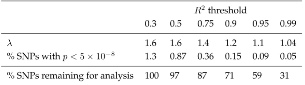
Table 1.1: Among SNPs genotyped in the Illumina controls and imputed using soft calls among the Affy controls, values ofλand percentages of SNPs withp <5×10⁻⁸when we restrict to SNPs with imputation qualityR2larger than the given thresholds, as detailed in Method 2. Also listed are the percentages of total SNPs remaining for analysis at each threshold.
R2threshold
0.3 0.5 0.75 0.9 0.95 0.99
λ 1.6 1.6 1.4 1.2 1.1 1.04
% SNPs withp <5×10⁻⁸ 1.3 0.87 0.36 0.15 0.09 0.05 % SNPs remaining for analysis 100 97 87 71 59 31
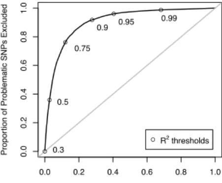
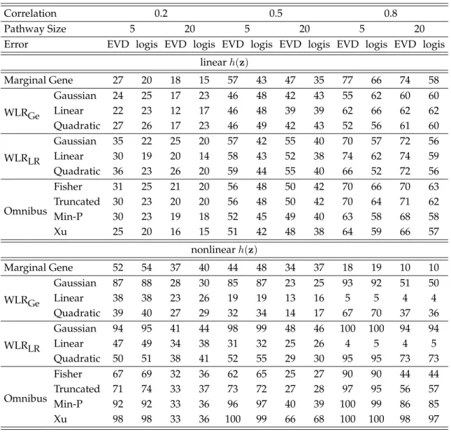
reflects some loss of power. It should also be noted that even at the most stringent threshold listed,R2 > 0.99,when we’ve excluded nearly 70% of the SNPs, there remain 57 SNPs withp < 5×10⁻⁸. Figure 1.3 shows the discriminatory ability of this method as we vary theR2threshold.
0.0 0.2 0.4 0.6 0.8 1.0 0.0 0.2 0.4 0.6 0.8 1.0
Proportion of Non−Problematic SNPs Excluded
Propor tion of Prob lematic SNPs Excluded ! ! ! ! ! ! 0.99 0.95 0.9 0.75 0.5 0.3 ! R2 thresholds
Figure 1.3: Among SNPs genotyped in the Illumina controls and imputed using soft calls among the Affy controls, discrimination of theR2criterion described in Method 2, as theR2-threshold varies. They-axis is the sensitivity, the proportion of highly significant SNPs which are excluded; thex-axis is1−specificity, the proportion of non-significant SNPs which are excluded.R2threshold choices between 0.3 and 0.99 are pointed out along the curve.
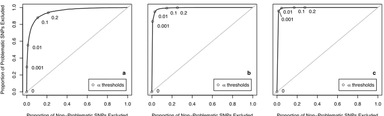
1.3.3 Method 3
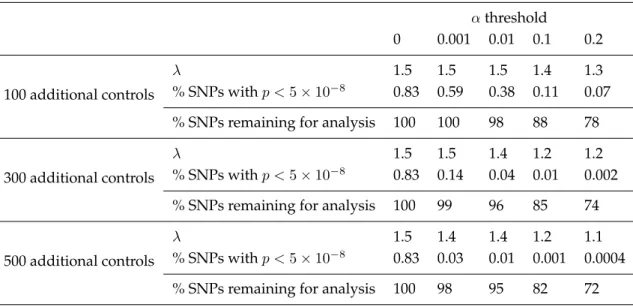
For various thresholds (α = 0.001,0.01,0.1,0.2) and various numbers of additional controls on Affy (n= 100,300,500) we removed SNPs significant at levelαin a preliminary analysis comparing then addi-tional Affy controls to the 1000 original Illumina controls. We then performed standard logistic regressions comparing the 1000 Illumina controls to the 1000 Affy cases using the remaining SNPs. The genomic con-trolλand the percentage of highly significant SNPs were calculated; results for the soft call genotypes are
shown in Table 1.2. Asnincreased andαincreased, our summary measures improved. This again
hap-pened at the expense of losing SNPs for analysis, but not as quickly as in Method 2. Figure 1.4 shows the discriminatory ability of this method for eachnas we vary theαscreening threshold.
Table 1.2: Results from the main analysis comparing 1000 Affy cases and 1000 Illumina controls, among SNPs remaining after a preliminary screen in which we comparen= 100,300,or500additional controls on Affy to 1000 controls on Illumina and remove SNPs significant at levelα,as detailed in Method 3. Among SNPs genotyped in the Illumina controls and imputed using soft calls among the Affy controls, values of
λand percentages of SNPs with p < 5×10⁻⁸ are presented, along with the percentages of total SNPs remaining for analysis at each threshold.
αthreshold
0 0.001 0.01 0.1 0.2 100 additional controls
λ 1.5 1.5 1.5 1.4 1.3
% SNPs withp <5×10⁻⁸ 0.83 0.59 0.38 0.11 0.07 % SNPs remaining for analysis 100 100 98 88 78 300 additional controls
λ 1.5 1.5 1.4 1.2 1.2
% SNPs withp <5×10⁻⁸ 0.83 0.14 0.04 0.01 0.002 % SNPs remaining for analysis 100 99 96 85 74 500 additional controls
λ 1.5 1.4 1.4 1.2 1.1
% SNPs withp <5×10⁻⁸ 0.83 0.03 0.01 0.001 0.0004 % SNPs remaining for analysis 100 98 95 82 72
0.0 0.2 0.4 0.6 0.8 1.0 0.0 0.2 0.4 0.6 0.8 1.0
Proportion of Non−Problematic SNPs Excluded
Propor tion of Prob lematic SNPs Excluded ! ! ! ! ! 0.2 0.1 0.01 0.001 0 ! ! thresholds a 0.0 0.2 0.4 0.6 0.8 1.0
Proportion of Non−Problematic SNPs Excluded
! ! ! ! ! 0.2 0.1 0.01 0.001 0 !! thresholds b 0.0 0.2 0.4 0.6 0.8 1.0
Proportion of Non−Problematic SNPs Excluded
! ! ! ! ! 0.2 0.1 0.01 0 0.001 !! thresholds c
Figure 1.4: Among SNPs genotyped in the Illumina controls and imputed using soft calls among the Affy controls, discrimination of the preliminary screening criterion described in Method 3, as theα-threshold
varies. They-axis is the sensitivity, the proportion of highly significant SNPs which are excluded; thex-axis is1−specificity, the proportion of non-significant SNPs which are excluded. Plots shown are foran= 100, bn= 300, andcn= 500additional controls. αthreshold choices between 0.001 and 0.2 are pointed out
1.4 Discussion
We observed a large number of highly significant SNPs after imputation in a study comparing two healthy control groups genotyped on different platforms. Because both control groups are nested in the NHS and chosen using similar criteria, we expect no SNPs to significantly distinguish the two groups in the absence of measurement error, and we expect no differential population substructure. Thus, statistically significant SNPs are false positives, and must be due to genotyping or imputation error. Furthermore, because we see almost no inflation in Type I error among SNPs actually genotyped on both chips (Figure 1.1a), the false positives do not appear to result from genotyping error. Rather, the inflation in Type I error is seen among SNPs measured in one group and imputed in the other (and among SNPs imputed in both). In this setting, it would be detrimental to avoid imputation altogether since only about a quarter of the SNPs genotyped on each platform overlap, so that three-quarters of the SNPs on each chip would be unusable without any imputation. Thus, we need to understand the errors being introduced by imputation and attempt to control for them.
We believe that the inflation in Type I error is due to bias introduced by the differential imputation. The imputation uses individuals in the HapMap as a reference panel, and it seems plausible that estimates in the HapMap, particularly for rare alleles, may diverge from the allele frequencies observed in our population. Thus, if a rare allele has similar frequencies in our cases and controls but is not well covered in the HapMap, thep-value calculated when the SNP is measured in one group and imputed in the other will tend to be smaller than thep-value that would arise if that SNP were measured in both groups. Moreover, among SNPs with low MAF, Moskvina et al. (2006) showed that even modest differential errors in genotype calling can yield an inflation in Type I error. Generalized to our setting, this suggests that even slight differential errors in imputation among SNPs with low MAF would lead to false positive associations. This is borne out by our results, where we see larger numbers of highly significantp-values among SNPs with low MAF, as shown in Figure 1.1.
The percentage of highly significant SNPs is noticeably larger in the hard call analysis than in the soft call analysis. This is because the soft call imputations better account for uncertainty in the imputed values. We recommend using soft calls, or another technique that accounts for imputation uncertainty, in order to reduce false positives. It is worth considering whether we could somehow alter the imputation methods themselves to avoid these false positives altogether; however, it is unclear to what extent this is
possible. Imputation algorithms are limited by the information they are provided. For some platforms, the genotyped SNPs provide enough information to accurately infer an unobserved SNP; for other platforms, they do not, regardless of the imputation algorithm. Moreover, current imputation methods have good accuracy, particularly for SNPs with higher imputationR2 (Li et al., 2010), yet even SNPs with high R2 appear among our false positives. This suggests that even well-imputed SNPs can be falsely significant when the imputation error is differential.
The inflation in Type I error appears to be most dramatic among SNPs measured in Illumina and imputed in Affy. We suspect that this is because Illumina uses HapMap for SNP selection, and we used HapMap for SNP imputation. When we considered SNPs common to both chips, the distribution of test statistics was what we expect under the null, suggesting that the actual genotyping across the two chips is in good agreement.
When we attempted to reduce the error inflation using PCs, in Method 1, we observed a complete sep-aration of the two control groups. This complete sepsep-aration shows the difficulty of controlling for platform effect by simply adjusting for PCs. Including the PCs as covariates in the model is equivalent to includ-ing case-control status as a covariate, and thus there does not appear to be a direct way to use those PCs to resolve the error inflation problem. Furthermore, any method using the PCs would likely wash out all differences between cases and controls in a non-null setting. Thus, it makes sense to focus on approaches that filter out problematic SNPs and exclude them from subsequent analysis. Methods 2 and 3 are two such approaches.
In Method 2, we used imputation quality to filter SNPs before performing any association tests. This approach improved the results and does not require genotyping any additional controls. It reduces the number of SNPs available for analysis, but still allows the use of more SNPs than just those actually geno-typed on both platforms. However, in our example of SNPs genogeno-typed on Illumina and imputed on Affy, even after filtering to SNPs imputed withR2 >0.99(allowing us to retain only 30% of SNPs), we are left with 57 SNPs with highly significantp-values out of 112,249 remaining SNPs. So if this method is used, researchers should be prepared to sift through many false positives in a second stage analysis to find any true associations. Furthermore, this method will tend to reduce power to detect SNPs in regions with low linkage disequilibrium. Beecham et al. (2010) demonstrated this problem by pooling two case-control GWA studies for Alzheimer disease which had been genotyped on different chips, and testing for associations in theAPOEgene, which is known to be strongly associated with risk. They used imputation to produce
com-mensurable data sets, and filtered out SNPs according to imputation quality. They found that even though each study separately found strong associations in theAPOEgene, there was no association in the pooled analysis, because many SNPs had been excluded due to low imputation quality measures caused by weak linkage disequilibrium in the region.
In Method 3, we propose genotyping a small number of additional controls alongside the cases and performing a preliminary step of filtering SNPs by comparing these additional controls to the original controls. This approach also improves results, but at increased monetary cost. It should, however, retain more non-artifactual SNPs while reducing the number of artifactual SNPs. In our example of 1000 cases and 1000 controls, it appeared that genotyping 300 additional controls alongside cases would allow researchers to filter out most of the false positives — withα= 0.2,only 5 highly significant SNPs were left among the SNPs genotyped on Illumina and imputed on Affy, with 264,519 (74%) remaining for analysis. We believe these results would be the same if we had new cases and controls on Illumina and a separate control group on Affy — we merely consider this setting because it made best use of the subjects available on each chip. This method is in line with the discussion in McCarthy et al. (2008) regarding the use of historical controls. McCarthy et al. listed many possible sources of systematic error that might arise in the use of historical controls, and recommended always genotyping some ethnically matched controls alongside cases on the same platform.
It may also be worth considering a related study design in which very little error inflation was seen, which was considered by Howie et al. (2009). In their setting, a central control group in the WTCCC was genotyped on both Affy and Illumina, while different case groups from different disease studies were geno-typed on just one of these platforms. The authors were interested in whether imputing SNPs missing in cases using both the HapMap and the central control group as a reference panel led to inflated Type I er-ror. To assess this, they compared the central control group with another control group genotyped on Affy alone. They imputed SNPs missing in this new control group and then performed association tests. They found very few significant results, which demonstrated minimal inflation of Type I error in this setting. Their methods differ slightly from ours; however, we believe that the most important difference was the nested structure of their design – that is, that their central control group had SNPs from both Affy and Illumina chips, rather than Illumina alone. A comparison of their results and ours suggests that if a central control group is going to be reused for different diseases, it may be wise to invest in genotyping the central control group on multiple platforms. A similar conclusion is offered by Marchini and Howie (2010).