Dept. of Math. University of Oslo Statistical Research Report No 1 ISSN 0806–3842 March 2011
A BAYESIAN HYPOTHESIS TESTING APPROACH FOR FINDING UPPER BOUNDS FOR PROBABILITIES THAT PAIRS
OF SOFTWARE COMPONENTS FAIL SIMULTANEOUSLY
MONICA KRISTIANSEN∗ Østfold University College
1757 Halden, Norway [email protected]
RUNE WINTHER Consultant at Risikokonsult
Oslo Area, Norway [email protected]
BENT NATVIG Department of Mathematics University of Oslo, Norway
Received (18 March 2011)
Predicting the reliability of software systems based on a component-based approach is inherently difficult, in particular due to failure dependencies between software compo-nents. One possible way to assess and include dependency aspects in software reliability models is to find upper bounds for probabilities that software components fail simulta-neously and then include these into the reliability models. In earlier research, it has been shown that including partial dependency information may give substantial improvements in predicting the reliability of compound software compared to assuming independence between all software components. Furthermore, it has been shown that including de-pendencies between pairs of data-parallel components may give predictions close to the system’s true reliability. In this paper, a Bayesian hypothesis testing approach for find-ing upper bounds for probabilities that pairs of software components fail simultaneously is described. This approach consists of two main steps: 1) establishing prior probability distributions for probabilities that pairs of software components fail simultaneously and 2) updating these prior probability distributions by performing statistical testing. In this paper, the focus is on the first step in the Bayesian hypothesis testing approach, and two possible procedures for establishing a prior probability distribution for the probability that a pair of software components fails simultaneously are proposed.
Keywords: Compound software; component dependencies; Bayesian hypothesis testing; expert judgment; prior information.
∗Corresponding author.
1. Introduction
The problem of assessing reliability of software has been a research topic for more than 30 years, and several successful methods for predicting the reliability of an individual software component based on testing have been presented in Frankl et al.13, Goel14, Hamlet19, Lyu40, Miller et al.42, Musa44, Ramamoorthy and
Bas-tani51, and Voas and Miller59. However, there are still no methods fully successful
for predicting reliability of compound software a based on reliability data on the
system’s individual software components15,17,60.
1.1. Motivation
For hardware, even in critical systems, it is accepted to base the reliability as-sessment on failure statistics, i.e. to measure the failure probability of individual hardware components and then compute system reliability on this basis. This is applied for example in safety instrumented systems in petroleum 22. However, the
characteristics of software make it difficult to carry out such a reliability assess-ment. Software is not subject to aging and any failure that occurs during operation is due to faults that are inherent in the software from the beginning. Any random-ness in software failure is due to randomrandom-ness in input data. It is also a fact that environments such as hardware, operating system and user needs change over time and that software reliability may change over time due to these activities9.
Furthermore, having a system consisting of several software components b
ex-plicitly requires an assessment of the software components’ failure dependenciesc.
This is discussed more thoroughly in, among others, Cortellessa and Grassi7, Dai
et al.10, Gokhale and Trivedi16, Guo et al.18, Littlewood et al.38, Lyu 40, Nicola and Goyal 46, Popic et al.49, Popov et al.50, and Tomek et al.56. In addition to
the fact that software reliability assessment is inherently difficult due to software complexity and that software is sensitive to changes in usage, failure dependencies between software components represent a substantial problem.
Although several different approaches to construct component-based software reliability models have been proposed in, among others, Cortellessa and Grassi7,
Gokhale and Trivedi 15, Gokhale 16, Goseva-Popstojanova and Trivedi 17, Ham-let20,21, Krishnamurthy and Mathur25, Krka et al. 32, Kuball et al. 33, Popic et
al.49, Reussner et al.52, Singh et al.54, Trung and Thang57, Vieira and Richard-son 58, and Yacoub et al.61, most of these approaches tend to ignore failure
de-pendencies between software components 11,24,36. In principle, the failure
proba-bility of a single software component can be assessed through statistical testing
12,53. However, since critical software components usually have low failure
proba-bilities 38, in practice the number of tests required to obtain adequate confidence aSoftware systems consisting of multiple software components.
bSee Definition 1 in Subsection 1.2. cSee Definition 2 in Subsection 1.2.
in such probabilities becomes very large. An even more non-trivial situation arises when probabilities for simultaneous failuresdof several software components need to be assessed, since they are likely to be significantly smaller than single failure probabilities.
Based on the fact that software components rarely fail independently and that statistical testing (for assessing the probability for software components failing si-multaneously) is practically impossible, the main focus of our research has been to develop a practicable component-based approach for assessing reliability of com-pound software in which failure dependencies between software components are explicitly addressed27,28,29,30,31.
One possible way to assess and include dependency aspects in software reliabil-ity models is to find upper bounds for probabilities that software components fail simultaneously and then include these into the reliability models. In Kristiansen et al.29 it is shown that including partial dependency information may give
substan-tial improvements in the reliability predictions of compound software compared to assuming independence between all software components. Furthermore, it is shown that including dependencies between pairs of data-parallel componentse may give
predictions close to the true system reliability. It is also shown that dependencies between pairs of data-parallel components are far more important than dependen-cies between pairs of data-serial componentsf.
In this paper, the theory on how to apply Bayesian hypothesis testing 8,26,55
to find upper bounds for probabilities that pairs of software components fail si-multaneously is described in detail. This approach can be divided into two main steps. In the first step, prior probability distributions for probabilities that pairs of software components fail simultaneously are established. In the second step, these distributions are updated by performing statistical testing. In this paper, two pos-sible procedures for establishing a prior probability distribution for the probability that a pair of software components fails simultaneously are proposed.
1.2. Definitions
In this paper, the following definitions are used:
Definition 1. Software component: a software component (or module or unit) is considered to be an entity that has a predefined and specified boundary and which is atomic in the sense that it can not or will not be divided into sub-components. No special assumptions are made whether the component is available in binary format or as source code. The context is essentially an Off-The-Shelf (OTS) situation where custom-developed and PDS componentsg are combined to achieve a larger piece of
software.
dSee Definition 3 in Subsection 1.2. eSee Definition 4 in Subsection 1.2. fSee Definition 5 in Subsection 1.2. gSee Definition 6 in Subsection 1.2..
Definition 2. Failure dependency between software components: compo-nents are said to fail dependently if the knowledge that one software component has failed changes our belief whether or not another software component fails60. It
is necessary to make a clear distinctions between thedegree of dependencybetween software components (expressed through e.g. simultaneous failure probabilities) and the mechanisms that either cause or exclude software components to fail depen-dently (interface complexity, shared resources, programming language, development team, etc.)
Definition 3. Simultaneous failure: the event that more than one software component fails on the same system input. Component failures are not required to occur at the same instant, it is adequate that they are all in a failed state at some point in time.
Definition 4. Data-parallel components: two componentsi andj are said to be data-parallel components if neitherinorjreceives data (d), directly or indirectly through other components, from the other29.
i9d j and j 9d i (1)
Definition 5. Data-serial components: two components i and j are said to be data-serial components if either i or j receives data (d), directly or indirectly through other components, from the other29.
i→d j or j →d i (2)
Definition 6. Pre-developed software (PDS): software which already exists, is available as commercial or proprietary product and is being considered for use in a computer-based system 1. This definition encompasses any kind of reuse of
software whether it is black-box, commercially available, from an in-house library, or just happens to be available from another system.
1.3. Assumptions
In this paper, only on-demand types of situations are considered, i.e. situations where the system is given an input and execution is considered to be finished when a corresponding output has been produced. The following assumptions are made:
• The states of the software components are positively correlated.
• All data-flow relations between the software components are known.
• The reliabilities of the individual software components are known.
• The system and its components have only two possible states (functioning and failed).
The research has been inspired by the following basic problem. Assume a compound software, e.g. a fault tolerant system capable of switching between two redundant software components in case of failure. Furthermore, assume that the failure prob-abilities of the individual software components are available. Even in this ideal situation, it is difficult to compute the failure probability of the complete system since no information regarding the failure dependencies between the software com-ponents is available. In this paper, the main focus is to include dependency aspects in software reliability models by applying Bayesian hypothesis testing.
1.4. Notation
In this paper, capital letters are used to denote random variables and lower-case letters are used for their realizations.
To indicate the state of the ith component, a binary value xi is assigned to componenti2.
xi=
0 if componentiis in the failed state
1 if componentiis in the functioning state (3)
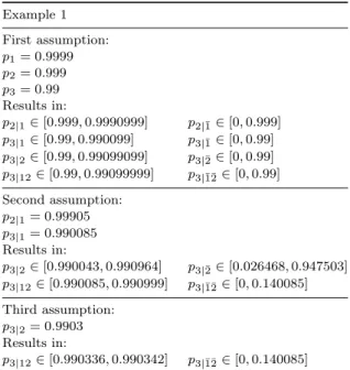
Important notation used throughout this paper is listed in Table 1.
1.5. The structure of this paper
Section 2 summarizes some related work regarding the issue of failure depen-dency between software components. In Section 3, relevant background information needed to understand the Bayesian hypothesis testing approach and our overall ap-proach for assessing reliability of compound software are described27. In Section 4,
a Bayesian hypothesis testing approach for finding upper bounds for probabilities that pairs of software components fail simultaneously is illustrated. This approach consists of two main steps: 1) establishing prior probability distributions for proba-bilities that pairs of software components fail simultaneously and 2) updating these prior probability distributions by performing statistical testing. In Section 5, two possible procedures for establishing a prior probability distribution for the proba-bility that a pair of of software components fails simultaneously are proposed. In addition, relevant information sources which may influence this probability distri-bution are presented. Section 6 summarizes the results, discusses the assumptions made and presents ideas for further work.
2. Related work
Most research and discussions on software component dependency over the years are mainly related to software design diversity, especially to N-version program-ming where output is decided by a voter using the results from N components as input. The idea behindN-version programming is that by forcing various aspects
Table 1. Notation.
Term Explanation
n = number of tests
r = number of failures inntests
θ = an unknown quantity, for example the probability that a pair of software components fails simultaneously qij = the probability that a pair (i, j) of software components
fails simultaneously
q0,ij = an accepted upper bound forqi,j π(θ) = a prior probability distribution forθ
π(qij) = a prior probability distribution forqijdefined in the
sub-intervals [aij, q0,ij] and [q0,ij, bij]
g(qij) = a prior probability distribution forqijdefined in the
interval [aij, bij] D = sample information
π(θ|D) = a posterior probability distribution forθ π(qij|D) = a posterior probability distribution forqij
[aij, bij] = interval where the simultaneous failure probabilityqijis defined H0 = null hypothesis (aij≤qij≤q0,ij)
H1 = alternative hypothesis (q0,ij< qij≤bij)
B = Bayes factor
L(θ|D) = likelihood function
π0 = prior belief in the null hypothesis (P(H0) =P(aij≤qij≤q0,ij)) π1 = prior belief in the alternative hypothesis
(P(H1) =P(q0,ij< qij≤bij))
α0 = posterior belief in the null hypothesis (P(H0|D))
α1 = posterior belief in the alternative hypothesis (P(H1|D))
C0,ij = a given predefined confidence level for the simultaneous
failure probability of a pair (i, j) of software components (P(H0|D)≥C0,ij)
g0(qij) = a probability distribution describing how the prior mass
is spread out over the null hypothesis
g1(qij) = a probability distribution describing how the prior mass
is spread out over the alternative hypothesis α, β = parameters in the beta distribution
of the development process to be different, i.e. development team, methods, tools, programming languages, etc., the likelihood of having the same fault in several components would become negligible.
The hypothesis that independently developed components fail independently has been investigated from various perspectives. A direct test of this hypothesis was done in Knight and Leveson24where a total of 27 components were developed by different people. Although the results can be debated, this experiment indicated that assuming independence should be done with caution. The experiment showed that the number of tests for which several components failed was much higher than anticipated under the assumption of independence. While there are many different mechanisms that might cause even independently developed components to fail on the same inputs, it does not seem implausible that the simple fact that programmers are likely to approach a problem in much the same way causes them to make the
same mistakes and thus generates dependency between the components’ failure behavior.
A more theoretical approach on the same issue was presented in Eckhardt and Lee 11 and elaborated on a few years later in Littlewood and Miller 36. A more comprehensive discussion is provided in Littlewood et al.38.
In the Eckhardt and Lee model (EL-model) there are two basic sources of un-certainty: 1) the random selection of input from the space of all inputs and 2) the random creation of a component version from the population of all possible com-ponent versions that can be written. The key variable in the model is the difficulty function φ(x) defined to be the probability that a component version chosen at random fails on a particular input demandx. In other words, if many component versions are selected independently, the difficulty function is the proportion of these that fail on a particular input. The idea of the Eckhardt and Lee model is that the difficulty function generally takes different values for different inputs, representing the varying difficulty in correctly processing different inputs. The more difficult an inputxis, the greater is the chance that an unknown component version fails.
The main result in the EL-model is that independently developed component versions do not imply independent component versions. The key point is that as long as some inputs are more difficult to process than others, even independently de-veloped component versions fail dependently. In fact, the more the difficulty varies between the inputs, the greater is the dependence in failure behavior between com-ponent versions. Only in the special situation where all inputs are equally difficult, i.e. the difficulty functionφ(x) is constant for all x∈Ω, independently developed component versions fail independently.
The Littlewood and Miller model (LM-model) is a generalization of the EL-model in which different component versions are developed using diverse method-ologies. In this context, the different development methodologies might represent different development environments, different types of programmers, different lan-guages, different testing regimes, etc. Thus, a component version has a different probability of being developed under methodology A than under methodology B. If the methodologies are very diverse, one expects a component version with a high probability of being developed under one methodology to have a low probability of being developed under another.
The main result of the LM-model is that the use of diverse methodologies de-creases the probability of simultaneous failure of several component versions. In fact, they show that it is theoretically possible to obtain component versions which exhibit better than independent failure behavior. So while it is natural to try to justify an assumption of independence, it is worthwhile noticing that having inde-pendent component versions is not necessarily the optimal situation with regard to maximizing reliability.
The main problem with both the EL-model and the LM-model is that the predic-tions of these models are predicpredic-tions for an “average” multi-version development. These models consider all possible software realizations from the same
specifica-tion and say nothing about a particular pair of component versions. Thus, actual realizations may be different from these averages.
In Popov et al.50, the authors extend the previous conceptual models proposed
in Eckhardt and Lee 11 and Littlewood and Miller36 and address the problem of assessing the reliability of a specific set of component versions. All their models refer to the simplest possible diverse-redundant configuration, i.e. two component versions (AandB) with perfect adjudication (1-out-of-2 system). This means that the system behaves correctly provided that either A or B behaves correctly. In Popov et al.50, the upper bounds are based on knowledge on the input space of the component versions. For each sub-domainSi(i= 1, . . . , n), the authors assume that the probabilityP(Si) of drawing a random input fromSi is known. Furthermore, they assume that the failure probabilities of component versionsAandBfor inputs from each sub-domainSi (PA|Si andPB|Si) are known.
If it is assumed that component versions fail independently within each sub-domain, the probability of simultaneous failure between component versions on a random input can be calculated directly from the known probabilities, i.e.
PA,Bsub−ind = PiPA|SiPB|SiP(Si). This estimate is an intermediate value be-tween the true failure probability (PA,B) and the failure probability one gets when assuming independence between the two component versions, i.e. PAPB. In fact, assuming conditional independence of failures within sub-domains is therefore less optimistic than assuming unconditional independence of the whole input space.
In Littlewood et al.37, the problem of assessing reliability of a 1-out-of-2
sys-tem is also considered. To do this, the authors apply Bayesian inference which includes establishing a prior belief regarding the parameters of interest and then updating these by using Bayes theorem when “hard” evidence becomes available. assuming that A and B are two diverse components, calculation of the system reliability requires that the probabilities PA = P(Afails), PB = P(B fails) and
PAB =P(BothA andB fails) are determined. This means that the degree of de-pendence between software components is implicitly addressed through PAB.
In the most general case, the authors’ propose that a 3-dimensional prior must be determined for the three probabilities which is conceptually and practicably very hard. In the less difficult situation where both PA andPB are assumed to be known, the authors run into a paradox where the posterior probability of system failure becomes higher than the prior probability when no component failures are observed during testing. The reason for this paradox is that the probability of having no failure in any of the components, i.e. 1−PA−PB+PAB is large if the probability PAB is also large. Hence, in practice it seems that neither the ”full” approach where all the relevant probabilities are handled simultaneously, nor the simplified approach where two out of three probabilities are assumed to be known work.
While the work of Littlewood et al.37 focuses on all three failure probabilities PA,PB andPAB, we solely focus onPABand suggest a Bayesian hypothesis testing approach to find upper bounds for probabilities that pairs of software components
fail simultaneously. This approach uses all relevant information which is available prior to testing and consists of the following main steps:
1. Establishing prior probability distributions for probabilities that pairs of software components fail simultaneously based on all relevant information available prior to testing (Section 5).
2. Updating these prior probability distributions by performing statistical testing (Section 4).
3. Theoretical background
In this section, relevant background information on statistical testing and Bayesian analysis is described in detail. In addition, it is shown how failure probabilities of individual components and the assumption of positive correlation put direct restrictions on the components’ simultaneous failure probabilities. All this informa-tion is needed to understand the Bayesian hypothesis testing approach for finding upper bounds for probabilities that pairs of software components fail simultane-ously. At last, our approach for assessing the reliability of compound software is described in detail27. In this approach, failure dependencies between pairs of soft-ware components are explicitly addressed by applying Bayesian hypothesis testing on simultaneous failure probabilities.
3.1. Statistical testing
Statistical testing12,53 consists of exposing a piece of software to test cases drawn
randomly according to some probability distribution defined over the program’s input space. Such testing can be used to assess a software component’s failure probability. Typical assumptions in statistical testing are: i) independent test runs, ii) constant failure rate, iii) all failures during testing are detected and iv) the operational profile is known.
One benefit of statistical testing is that it requires no knowledge of the internal structure of the software components being tested. This is of great importance when PDS componentsh are used, for which one might not have all the required
information available.
Letp0 denote the accepted upper failure probability. The number of fault free
tests n which must be carried out to satisfy the failure probability p0 at a given
confidence levelC0using classical statistical testing is given in Equation 4 48.
n= ln(1−C0)
ln(1−p0)
(4)
3.2. Bayesian analysis
Bayesian analysis3consists of combining prior informationπ(θ) and sample
infor-mationDinto a posterior distributionπ(θ|D) forθgiven D. It is from this posterior distribution all decisions and inferences are made in Bayesian analysis. Bayes the-orem 3is expressed in Equation 5 where the prior distributionπ(θ) reflects beliefs
aboutθprior to testing and the posterior distribution π(θ|D) reflects updated be-liefs about θ after testing. L(θ|D) is the likelihood function which expresses the likelihood ofθ given sample informationD.
π(θ|D) =R L(θ|D)π(θ) ΘL(θ|D)π(θ)dθ
(5) In hypothesis testing, a null hypothesis (H0) and an alternative hypothesis (H1)
are specified. In classical statistics, one decides between H0 and H1 by examining
type I and type II error probabilities. These probabilities of error represent the chance that for an observed sample the test procedure results in the wrong hy-pothesis being accepted. Type I error occurs when H0 is rejected when it is true
and type II error occurs when H0 is accepted when it is false. In Bayesian
anal-ysis, hypothesis testing is conceptually more straightforward. One calculates the posterior probabilitiesα0=P(H0|D) andα1=P(H1|D) which combine both test
data and prior knowledge and then decide betweenH0andH1accordingly3. Often
it is convenient to summaries the evidence in term of posterior odds. Saying that
α0/α1 > R clearly says that H0 is R times as likely to be true as H1. Although
the posterior probabilities of the hypotheses are the primary measures in Bayesian hypothesis testing, the prior probabilities π0=P(H0) andπ1 =P(H1) are also of
interest. The ratioπ0/π1 is called the prior odds ratio and the Bayes factor can be
expressed by combining the prior and posterior odds ratios (see Equation 6).
B= α0/α1
π0/π1
=α0π1
α1π0
(6) The Bayes factor is the odds ratio for H0 to H1 that is given by the data 3. If
the Bayes factor is greater than one, data helped increasing odds in favor of the null hypothesis8. The Bayes factor forms the basis for finding the number of tests required to satisfy a predefined upper bound q0,ij at confidence level C0,ij in the proposed approach for finding upper bounds for probabilities that pairs of software components fail simultaneously. This approach is elaborated in detail in Section 4.
3.3. Prior Information from the Software Components’ failure probabilities
In this section, it is illustrated how the software components’ marginal failure proba-bilities put direct restrictions on the components’ simultaneous failure probaproba-bilities. Letqiandqjdenote the failure probability of componentsiandj, respectively, and
letqij denote the simultaneous failure probability of componentsiandj. If it can be assumed that the components’ failure probabilities do not change due to changes in operational context, the following is true:
qij≤min(qi, qj), (7)
which follows directly from the fact that:
qij =P(Xi= 0∩Xj = 0) =P(Xi= 0)P(Xj = 0|Xi= 0)
=P(Xj= 0)P(Xi= 0|Xj= 0). (8) In general, one would expect positive correlation between componentsiandjsince some inputs are more difficult (more error-prone) than others 38. Even if diverse components are produced “independently”, failures are more likely to happen on certain inputs than others. This means that if componentifails, the failure proba-bility of componentj will also increase. However, when components are in parallel this may not always be a reasonable assumption. If components have been devel-oped by different development teams and by using different development methods and languages, it might in fact be natural to assume negative correlation. This means that if one component fails, the failure probability of the other component decreases and visa versa. However, assuming positive correlation is far more con-servative than assuming independence between software components when it comes to predicting system’s reliability. It follows that:
qij≥qiqj. (9)
Reasonable constraints on the simultaneous failure probabilityqij under the given assumptions can therefore be expressed as follows:
qiqj ≤qij ≤min(qi, qj). (10)
From Equation 10, it can be clearly seen that information on the software compo-nents’ marginal failure probabilities can be used directly to specify the upper and lower limit for the simultaneous failure probabilityqij. In the following, these limits will be used to:
• specify the hypotheses in the component-based approach (Subsection 3.4 and Section 4).
• specify a starting point when establishing a prior probability distribution for the simultaneous failure probabilityqij (Section 5).
The topic on how the reliabilities of individual software components put direct restrictions on the components’ conditional reliabilities is elaborated in more de-tail in Kristiansen et al. 29. In this paper, the authors present restrictions on the
0.0 0.2 0.4 0.6 0.8 1.0 0.9990 0.9994 0.9998 a) p2||1 p2|| 1 0.0 0.2 0.4 0.6 0.8 1.0 0.9990 0.9994 0.9998 b) p2||1 0.0 0.2 0.4 0.6 0.8 1.0 0.9990 0.9994 0.9998 c) p2||1
Fig. 1. Possible values for the conditional reliabilities in a two components system when a) p1= 0.999 andp2= 0.999, b)p1= 0.999 andp2= 0.9999 and c)p1= 0.9999 andp2= 0.999.
Examples of how the marginal reliabilitiesp1andp2influence the conditional
relia-bilitiesp2|1andp2|¯1in a general two components system are illustrated in Figure 1.
The graphs clearly show that the restrictions on the conditional reliabilities de-pend heavily on the values of the marginal reliabilities. In fact, in some cases the conditional reliabilities are restricted into narrow intervals.
In the same way, it is shown how the marginal reliabilitiesp1,p2, andp3influence
the conditional reliabilitiesp2|1,p2|¯1,p3|1,p3|¯1,p3|2,p3|¯2,p3|12andp3|¯1¯2in a general
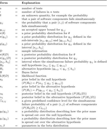
three components system. An example is illustrated in Table 2 which should be read
Table 2. Restrictions on the conditional reliabilitiesp2|1,
p3|1,p3|2 andp3|12in a simple three components system whenp1= 0.9999,p2= 0.999 andp3= 0.99. Example 1 First assumption: p1= 0.9999 p2= 0.999 p3= 0.99 Results in: p2|1∈[0.999,0.9990999] p2|¯1∈[0,0.999] p3|1∈[0.99,0.990099] p3|¯1∈[0,0.99] p3|2∈[0.99,0.99099099] p3|¯2∈[0,0.99] p3|12∈[0.99,0.99099999] p3|¯1¯2∈[0,0.99] Second assumption: p2|1= 0.99905 p3|1= 0.990085 Results in: p3|2∈[0.990043,0.990964] p3|¯2∈[0.026468,0.947503] p3|12∈[0.990085,0.990999] p3|¯1¯2∈[0,0.140085] Third assumption: p3|2= 0.9903 Results in: p3|12∈[0.990336,0.990342] p3|¯1¯2∈[0,0.140085]
as follows:
• In the first assumption it is assumed that the marginal reliabilities of the components are known. Knowing these reliabilities puts direct restrictions on all the remaining conditional reliabilities. In some cases they limit the conditional reliabilities into small intervals.
• In the second assumption it is assumed that the conditional reliabilities
p2|1andp3|1 are known in addition to the marginal reliabilities. This puts
even more strict restrictions on the remaining conditional reliabilitiesp3|2, p3|¯2,p3|12 andp3|¯1¯2.
• In the third assumption the conditional reliabilityp3|2is also assumed to be
known and it can be easily seen that the more information that is available, the more strict are the restrictions on the remaining reliabilitiesp3|12 and p3|¯1¯2.
3.4. A component-based approach for assessing the reliability of compound software
The main focus of our research has been to develop a component-based approach for assessing reliability of compound software where failure dependencies between software components are addressed explicitly 27. One possible way to assess and
include dependency aspects in software reliability models is to find upper bounds for probabilities that pairs of software components fail simultaneously and then include these into the reliability models. To find these upper bounds, the suggested approach applies Bayesian hypothesis testing8,26,55on simultaneous failure probabilities (see
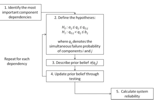
Section 4 for details). It is assumed that failure probabilities of individual software components are known. The approach is illustrated in Figure 2 and consists of five basic steps.
1. Identify the most important component failure dependencies: based on the structure of the software components in the compound software and infor-mation regarding individual software components, identify those dependen-cies between pairs of software components which are of greatest importance for the calculation of the system reliability29. Repeat steps 2-4 for all
rel-evant component dependencies in the system.
2. Define the hypotheses: letq0,ij represent an accepted upper bound for the probability (qij) that a pair (i, j) of software components fail simultane-ously. The upper boundq0,ij is assumed to be context specific and prede-fined and is typically derived from standards, regulation authorities, cus-tomers, etc. Define the following hypotheses:
H0:aij ≤qij ≤q0,ij
Fig. 2. A component-based approach for assessing the reliability of compound software.
whereqij is defined in the interval [aij, bij]. The interval limitsaij andbij represent the lower and upper limit forqij, respectively and are decided by the restrictions that the components’ marginal failure probabilities put on the components’ simultaneous failure probabilities (Subsection 3.3). 3. Describe prior belief regarding probability qij: establish a prior probability
distributionπ(qij) for the probability that a pair of software components fail simultaneously. Based on this probability distribution the prior belief in the null hypothesis (P(H0)) must be quantified.
4. Update your belief in hypothesis H0: based on the prior belief in the null
hypothesisP(H0) from step 3 and a predefined confidence levelC0,ij, the number of tests required to obtain an adequate upper bound for the proba-bility of simultaneous failure can be found for different numbers of failures
rencountered during testing. The more failures that occur during testing, the more tests are required to reachC0,ij. For further details on when to
stop testing see Section 4 or Cukic et al.8.
5. Calculate the complete system’s failure probability: information regarding individual software components’ failure probabilities (which are assumed to be known) and upper bounds for the most important simultaneous fail-ure probabilities (found in step 1-4) can finally be combined to obtain an upper bound for the failure probability of the entire system. This can be performed by various methods, e.g. by discrete event simulation when di-rect calculation becomes too complicated.
Step 1 in the component-based approach has been discussed in Kristiansen et al.29.
In that paper, a test system consisting of five components is investigated to iden-tify possible rules for selecting the most important component dependencies. To do this, three different techniques are applied: 1) direct calculation, 2) Birnbaum’s importance measure of a component and 3) Principal Component Analysis (PCA). The results from the analyses clearly show that including partial dependency infor-mation may give substantial improvements in the reliability predictions compared to assuming independence between all software components. However, this is only true as long as the most important component dependencies are included in the reliability calculations. It is also apparent that dependencies between pairs of data-parallel components are far more important than dependencies between pairs of data-serial components. Furthermore, the analyses indicate that including only de-pendencies between pairs of data-parallel components may give predictions close to the system’s true failure probability as long as the dependency between the most unreliable components is included. Including only dependencies between pairs of data-serial components may however result in predictions even worse than by assuming independence between all software components.
Step 3 in the component-based approach has been discussed in Kristiansen et al.31. In that paper, the results from an experimental study which investigates the relations between a set of internal software metrics (McCabe’s cyclomatic complex-ity, Halstead metrics, Source Lines of Code etc.) and stochastic failure dependency between software components are presented. The experiment was performed by an-alyzing a large collection of program versions submitted to the same specification in a programming competition on the Internet: the Online judgei. In the study, pairs of program versions were investigated. To measure the probability that a pair of program versions fails dependently, the study used the simultaneous failure proba-bility of the program versions. If any relations between the probabilities that pairs of software components fail simultaneously and their difference in software metrics can be identified, one possible step forward will be to use this information as prior information in the Bayesian hypothesis testing approach for finding upper bounds for simultaneous failures between pairs of software components. Results from uni-variate analyses show that if the difference between metric values of two program versions is small, it is impossible to decide the degree of failure dependency be-tween those two program versions. However, given that the metric values for a pair of program versions differ significantly and the program versions are reasonable mature, results indicate that the probability for simultaneous failures is less than the probability calculated if the metric values were similar.
In addition, a simulator which explicitly accounts for failure dependencies be-tween the software components and can be used to calculate the complete system’s failure probability when direct calculation becomes too difficult has been devel-ihttp://icpcres.ecs.baylor.edu/onlinejudge
oped. This simulator can be used in step 5 in the component-based approach and is described in Kristiansen et al.30.
The rest of the present paper focuses on steps 3 and 4 in the component-based approach and describes a Bayesian hypothesis testing approach for finding upper bounds for probabilities that pairs of software components fail simultaneously. First, the theory behind this approach is described in detail in Section 4. Then two pro-cedures for establishing a prior probability distribution for the probability that a pair of software components fails simultaneously are described in Section 5.
4. Bayesian hypothesis testing applied on simultaneous failure probabilities of pairs of software components
One possible approach to find upper bounds for probabilities that pairs of software components fail simultaneously is to use Bayesian hypothesis testing 8,26,27,55.
Assume thatH0 and H1 are defined as in step 2 in Section 3.4 where qij is a probability in the interval [aij, bij]. Here qij represents the probability that a pair (i, j) of software components fails simultaneously. The interval limits aij and bij represent the lower and upper limit for qij, respectively, and are decided by the restrictions the components’ marginal failure probabilities put on the components’ simultaneous failure probabilities as described in Section 3.3 (for more information see Kristiansen et al.29). In this case, the null and alternative hypotheses state that
the probability for a pair of software components to fail simultaneously is lower and higher than the given upper boundq0,ij, respectively.
Notice that the hypotheses are defined the opposite way of classical statistical hypothesis testing. In classical hypothesis testing, the alternative hypothesis usually expresses what one wishes to confirm, i.e. that the probability for simultaneous failure is less than a predefined upper bound q0,ij, whereas the null hypothesis is
the most conservative and expresses the opposite. In this way, the doubt benefits the null hypothesis which is true until the opposite is proved. However, by looking at the mathematics in the Bayesian hypothesis testing approach it can be easily seen that it does not matter which way the hypotheses are defined.
To express the prior belief in the simultaneous failure probabilityqij, two sep-arate probability distributions over the intervals [aij, q0,ij] and (q0,ij, bij] can be used3. This is expressed in Equation 11.
π(qij) =
P(H0)g0(qij)aij≤qij≤q0,ij
P(H1)g1(qij)q0,ij< qij ≤bij (11)
where g0(qij) and g1(qij) are proper probability density functions (g0(qij) > 0,
Rq0,ij
aij g0(qij)dqij = 1, g1(qij) > 0,
Rbij
q0,ijg1(qij)dqij = 1) which describe how the prior mass is spread out over the two hypotheses.
Letg(qij) be the prior probability distribution for qij in the interval [aij, bij]. The probability density functionsg0(qij) andg1(qij) can then be defined as shown
g0(qij) = 1 P(H0) g(qij) aij ≤qij ≤q0,ij (12) g1(qij) = 1 P(H1) g(qij) q0,ij < qij ≤bij (13) The probability distribution for observing r simultaneous failures during testing givennindependent trials and a constant simultaneous failure probability qij can be expressed by the binomial probability distribution. This is shown in Equation 14.
f(r|qij, n) =
n
r
qrij(1−qij)n−r (14)
The posterior belief in the null hypothesisH0is the probability of the null
hypoth-esis in light of data and prior knowledge. For acceptance, this probability must be higher than a given predefined confidence levelC0,ij.
P(H0|r, n)≥C0,ij (15)
The number of tests n required to satisfy the confidence level C0,ij for different numbers of simultaneous failures encountered r during testing can be found by using Bayes factor. Based on Equations 11 and 14, the posterior odds ratio can be expressed as shown in Equation 16.
α0 α1 = P(H0|r, n) P(H1|r, n) = Rq0,ij aij f(r|qij, n)P(H0)g0(qij)dqij Rbij q0,ijf(r|qij, n)P(H1)g1(qij)dqij (16) Further, it can easily be shown that the Bayes factor given by Equation 6 can be written as the weighted likelihood ratio as shown in Equation 17.
B = Rq0,ij aij f(r|qij, n)g0(qij)dqij Rbij q0,ijf(r|qij, n)g1(qij)dqij (17) Based on the acceptance criterion in Equation 15, it can be shown that the Bayes factor given in Equation 6 must satisfy Equation 188.
B≥ C0,ijP(H1)
(1−C0,ij)P(H0)
(18) The number of testsnrequired to obtain an adequate upper bound for the proba-bility that a pair of software components fails simultaneously for different numbers of simultaneous failuresrencountered during testing can be found by solving Equa-tion 19, which is based on EquaEqua-tions 17 and 18.
Rq0,ij aij f(r|qij, n)g0(qij)dqij Rbij q0,ijf(r|qij, n)g1(qij)dqij = C0,ijP(H1) (1−C0,ij)P(H0) (19) Equation 19 can be solved numerically by simply programming a loop which stops and returns the number of tests when the left side exceeds the right side in the equation. The integrals must be solved by using numerical integration.
5. Establishing prior probability distributions for probabilities that pairs of software components fail simultaneously
Before testing can be performed in the Bayesian hypothesis testing approach de-scribed in Section 4, a prior probability distribution g(qij) for the simultaneous failure probabilityqij defined in the interval [aij, bij] must be established. This dis-tribution is needed for establishingg0(qij) andg1(qij) in Equations 12 and 13 and
for calculating P(H0) andP(H1).
The main motivation for establishing a prior probability distribution for qij is to utilize all relevant information sources available prior to testing in order to compensate for the enormous number of tests which is usually required to satisfy a predefined confidence levelC0,ij. In the case where reasonable prior information
is available, the number of tests which must be run to achieveC0,ij in Equation 15 can be greatly reduced.
In the following, two procedures for establishing a prior probability distribution
g(qij) for the simultaneous failure probability qij are proposed. Both procedures consist of two main steps, the first step being common for both of them.
1. Establish a starting point forqij based on a transformed beta distribution. 2. Adjust this starting point up or down by applying expert judgment on
relevant information sources available prior to testing.
In the first procedure, the prior probability distribution for qij is determined by letting experts adjust the initial mean and variance ofqij in the transformed beta distribution based on relevant information sources. In the second procedure, the prior transformed beta distribution forqijis adjusted numerically by letting experts express their belief in the total number of tests and the number of simultaneous failures that all relevant information sources correspond to. A combination of these two procedures can also be applied, since it might be easier for experts to adjust the mean and variance for some information sources, whereas for other information sources it might be easier to express belief about the total number of tests and the number of simultaneous failures.
The challenge of using expert judgment for decision making and how to calibrate experts has been addressed in several books and papers, among others Clemen and Lichtendahl4, Cooke5, Cooke and Goossens6, Lin and Bier35, Meyer and Booker41 and Mosleh et al. 43. There is also a lot of research covering the psychological
and Plous47.
In the following subsection, ideas on how to establish a starting point for the si-multaneous failure probabilityqijare described. Then, two procedures for adjusting this starting point up or down based on relevant information sources and expert judgment are described in detail. Finally, a set of available information sources relevant for adjusting the starting point forqij is presented.
5.1. Establishing a starting point
As a basis for establishing a starting point for the simultaneous failure probability
qij, the following two assumptions are made:
1. The individual software components’ failure probabilities are available. 2. The components are positively correlated.
Additionally, if it can be assumed that the failure probabilities of the individual components do not change due to changes in the operational context, reasonable constraints on the simultaneous failure probability qij can be found as shown in Equation 10 in Section 3.3. Letaij =qiqj and bij =min(qi, qj) denote the lower and upper limit for the simultaneous failure probabilityqij, respectively. Under the assumption that the failure probabilities of the individual components do not change due to changes in the operational context, one possible way to identify the initial values of the mean and variance ofqijis to assume thatqijis uniformally distributed (beta distributed with parametersα=β= 1 over the interval [aij, bij]). The initial mean (µI) and variance (σI2) are then given by the following two equations:
µI = aij+bij 2 (20) σ2I = (bij−aij)2 12 (21)
However, since changes in the operational context are likely to change the failure probability of the individual components, a more conservative starting point is to usebij =min(qi, qj) as the initial mean. A possible set of initial values of the mean and variance of qij can therefore be given by:µI =bij and σI2 = (bij −aij)2/12. It is important to notice that these initial values are only a starting point for describing the simultaneous failure probability qij. These values and accordingly the resulting transformed beta distribution describingqij are adjusted by applying expert judgment on relevant information sources available prior to testing.
When the initial values of the mean and variance of qij in the transformed beta distribution are known, the initial values of the parametersαI and βI in the standard beta distribution can be found directly by applying linear transformation. This is shown in Equations 22 and 23.
µI =aij+ (bij−aij)
αI
αI+βI
σI2= (bij−aij)2
αIβI
(αI+βI)2(αI+βI + 1)
(23) Another possible way to identify initial values of α and β in the standard beta distribution is to visualize a “fictive” experiment in whichnI is the total number of experiments and αI is the number of simultaneous failures of components i and j. The simultaneous failure probability qij can then be assumed to have a transformed beta distribution with parametersαI andβI =nI−αI defined in the interval [aij, bij].
In addition to the the individual software components’ failure probabilities, in-formation regarding components’ architecture, complexity, programming languages, development processes, etc. might as well be available. This information is also rel-evant for assessing qij and can be used to adjust its starting point up or down by applying expert judgment. In the following two subsections, two procedures for ad-justing the starting point forqij up or down based on relevant information sources and expert judgment are described.
5.2. Establishing a prior probability distribution for qij by
adjusting its mean and variance
In the following section, a procedure on how relevant information sources can be used to adjust the initial mean µI and variance σ2I of the simultaneous failure probability qij in the transformed beta distribution is described. To illustrate this procedure, only two information sources are considered.
Define the following two information sources:
I1: Degree of complexity of the interface between the components.
I2: Degree of similarity between the programming languages of components iandj.
Assume that both information sources can be assigned values in the interval [0,1], such that a value close to 0 indicates low complexity (substantial difference in pro-gramming language) and a value close to 1 indicates extreme complexity (identical programming languages). In addition, let a value of 0.5 describe the “typical” sit-uation for the components under consideration.
Based on these two information sources, the following interpretations seem plau-sible:
1. I1andI2are both close to 0: the mean and variance of the prior distribution
are lower thanµI andσI2, respectively.
2. I1 and I2 are both close to 1: the mean of the prior distribution is larger
thanµI, while the variance is smaller thanσI2.
3. I1 is close to 0 andI2 is close to 1: the mean is dependent on the relative
4. I1 is close to 0.5 andI2 is close to 0: the mean of the prior distribution is
lower thanµI, and the variance is close toσI2.
In order to establish a prior probability distribution forqij, a functional relationship between the initial values defined byµI, σI2, all relevant information sources and the parametersαand β in the standard beta distribution must be defined.
Let Ii ∈ [0,1] denote information source i where i = 1, . . . , r, and let ki ∈ [0,1] express the relative importance of each information source. Furthermore, let
µdenote the adjusted mean ofqij andσ2the adjusted variance in the transformed beta distribution. A simplistic way to update the mean and variance using the information sources might then be as follows:
µ=2µI(k1I1+k2I2+· · ·+krIr)
k1+k2+· · ·+kr
(24)
σ2=σI2kV ar(I), (25)
whereV ar(I) is the sample variance calculated over the information sourcesIi, and
kis an impact factor that defines the impact the differences in theIivalues should have. The updated varianceσ2increases if there are large differences between the Ii’s (i.e. they give divergent information) and decreases if the differences between the Ii’s are small (i.e. they give similar information). Note that if Ii = 0.5 for
i= 1, . . . , n, thenµ=µI.
In the above procedure, both theIi’s,ki’s andkmust be determined by experts. Then when the updated values of the mean and variance are found, the parameters
αand β in the standard beta distribution can be found by solving Equations 22 and 23 by replacingαI byα,βI byβ,µI byµandσI2byσ2.
5.3. Establishing a prior probability distribution for qij by
adjusting it numerically
Based on the starting point established in Section 5.1, let us assume that the simul-taneous failure probabilityqij can be expressed by a transformed beta distribution with parametersαI andβI. In order to adjust this probability distribution, a func-tional relationship between the initial parameters defined by αI and βI and all relevant information sources must be defined.
As in Section 5.2, letIi denote a relevant information sourceiand letkiexpress the relative importance of this information source. Further, letn0andα0represent
the total number of tests and the number of simultaneous failures of componentsi
andj that all relevant information sources correspond to, respectively.
A possible way to findα0using all relevant information sources is expressed in
Equation 26.
α0=
n0(k1I1+· · ·+krIr)
k1+· · ·+kr
From this equation, it can be easily seen that the larger (closer to 1) the values of the relevant information sources Ii are, the larger is the number of simultaneous failures of components iandj.
The information achieved from all relevant information sources correspond to a binomial probability distribution with parametersα0andn0. Since the transformed
beta distribution with initial parametersαI andβI defined in the interval [aij, bij] lacks the pleasant property of being a natural conjugate prior to the binomial dis-tribution, the prior probability distribution for the simultaneous failure probability
qij must be adjusted numerically. In the above procedure theIi’s,ki’s andn0must
be determined by experts.
5.4. Relevant information sources used to adjust the starting point
In the following section, different types of information sources relevant for adjusting the starting point for the simultaneous failure probabilityqij are discussed.
Mechanisms that cause software components to fail simultaneously can be split into two distinct categories60:
• Development-cultural aspects (DC-aspects): mechanisms which cause dif-ferent people, tools, methods, etc. to make the same mistakes.
• Structural aspects (S-aspects): mechanisms which allow a failure in one component to affect the execution of another component.
The first category can typically be assessed using component specific information sourcesKi. On the other hand, the second category cannot be completely assessed using only component specific information. Information sources on how the com-ponents are used in a specific context or in the compound software (Kcompound) is also needed. While Ki might be viewed as generic information, meaning that it does not change when the use of the component changes,Kcompound is completely context-specific.
To successfully adjust the starting point forqij, the following information sources must be considered by experts9,34,62:
• The parts of a software component’s pedigree that are relevant to be com-pared with another software component’s pedigree, i.e. specific elements of
Ki for all componentsi. This may include:
– Development methodology.
– Programming language.
– Development team.
– Specification.
– Producer’s reputation.
– Software metrics (McCabe’s cyclomatic complexity, Halstead com-plexity measures, program depth, source lines of code (SLOC), number of comments and comment lines, number of loops and statements).
– Development tools (e.g. compiler).
– Previous testing
– Risk analysis methods.
– Standards.
– Software components’ history.
• The elements comprisingKcompound. This may include:
– Structural isolation of software components.
– Software component’s robustness.
– Sharing of resources (CPU, library routines, data memory, stack, op-erating system, etc.).
– How the software components are structurally related.
All these underlying information sources can possibly indicate if two software com-ponents are likely to fail simultaneously or not and can help experts to adjust the starting point for the simultaneous failure probability (qij) described in Subsec-tion 5.1.
Both procedures for adjusting the starting point described in Subsections 5.2 and 5.3 assume that relevant information sources can be assigned values in the interval [0,1]. A value close to 0 can for example indicate substantial difference in development methodologies, great diversity between development teams or low complexity of the interface between the software components. On the other hand, a value close to 1 can for example indicate use of identical development method-ologies, extreme complexity of the interface between the software components or that components are developed by the same development team. The idea is that the larger (closer to 1) the values of the relevant information sources Ii are, the larger is the meanµ for the simultaneous failure probability in the first procedure and the number of simultaneous failuresα0 in the second procedure.
A critical question is if experts are able to express their belief about relevant information sources using a numerical scale from 0 to 1. One possible simplification is to let experts express their beliefs on an ordinal scale first and then map this onto a numerical scale. For example, for a five point ordinal scale{very low, low, medium, high, very high}, “very low” can be associated with the interval [0,0.2), ”low” can be associated with the interval [0.2,0.4) and so on. Furthermore, the mean values in each interval can be used to perform the calculations in Equations 24 and 26.
6. Summary, discussion and further work
During development of the component-based approach for assessing reliability of compound software, two major challenges were identified:
1. How to identify those dependencies between pairs of software components that are of greatest importance for the calculation of the system reliability. This is necessary since it is not realistic to handle all possible dependencies in compound software.
2. How to establish prior probability distributions for probabilities that pairs of software components fail simultaneously.
Whereas the first challenge has been discussed in detail in Kristiansen et al. 27,29,
the main focus of this paper has been to describe the theory behind the Bayesian hypothesis testing approach for finding upper bounds for simultaneous failure prob-abilities (qij). This approach consists of two main steps:
1. Establishing prior probability distributions for probabilities that pairs of software components fail simultaneously.
2. Updating these prior probability distributions by performing statistical testing.
In this paper, two possible procedures for establishing a prior probability distribu-tiong(qij) for the simultaneous failure probability qij have been proposed. In the first procedure, the prior probability distribution for qij is determined by letting experts adjust the initial mean and variance of qij in the transformed beta distri-bution based on relevant information sources. In the second procedure, the prior transformed beta distribution for qij is adjusted numerically by letting experts express their belief in the total number of tests and the number of simultaneous failures that all relevant information sources correspond to.
By covering the second and last challenge in our approach, we finally come to the definition of a complete component-based approach for assessing reliability of compound software in which failure dependencies are explicitly addressed. To include dependency aspects in the reliability model, the approach uses information on the individual components’ failure probabilities (assumed to be known) and other relevant information sources available prior to testing. It should, however, be emphasized that the proposed procedures are only suggestions on how to find prior probability distributions for probabilities that pairs of software components fail simultaneously. The validation of these procedures has not yet been performed and is one of the main tasks for further work. Furthermore, testing the complete component-based approach on a realistic case will be prioritized.
The component-based approach for assessing reliability of compound software is based on a set of assumptions (see Subsection 1.3). In the following, a short discussion regarding these assumptions is given.
Positive correlation between two software components is normally expected es-sentially because some inputs are more difficult (more error-prone) than others. Even if two diverse software components are developed “independently”, failures are more likely to happen on certain inputs than on others. Assuming positive cor-relation is therefore rather realistic in many cases and far more conservative than assuming independence between software components when it comes to predicting the system’s reliability. In addition, recent calculations have shown that assuming positive correlation has only minor influence on the restrictions that the marginal component reliabilities put on the conditional reliabilities in a simple two com-ponents system. However, more research on systems consisting of more than two components is needed and will be carried out as further work.
It is natural to assume that some design documents defining the architecture, component interfaces and other characteristics of the system are available when a compound software is assessed. Structure charts which graphically show the flow of data and control information between components in a compound software are of special interest. They give an overview of the software structure and are funda-mental for identifying the most important component dependencies in the system, i.e. those dependencies that influence the system reliability the most.
Although the issue on how to predict reliability of individual software compo-nents is by no means trivial, our approach assumes that these probabilities are already known. How to assess these probabilities has been studied by several re-searchers over the years and an overview of different techniques for predicting the reliability of a particular software component based on testing can be found in, among others, Littlewood and Strigini39, Lyu40 and Musa44.
Assuming that the compound software is a monotone system and that the com-pound software and its components have only two possible states represents a limi-tation made to simplify our approach. Software components and compound software do usually have a number of possible failure modes and more research on how to include multiple failure modes is needed.
Acknowledgment
This work has been performed as part of a PhD-study in collaboration between Østfold University College and the University of Oslo.
References
1. IEC 60880-2:2000: Software for computers important to safety for nuclear power plants. Software aspects of defence against common cause failures, use of software tools and of pre-developed software. 2000.
2. T. Aven.Reliability and Risk Analysis. Elsevier, London, 1992.
3. J. O. Berger. Statistical Decision Theory and Bayesian Analysis. Springer Verlag,
second edition, 1985.
4. R. T. Clemen and K. C. Lichtendahl. Debiasing expert overconfidence: a Bayesian
calibration model.Working paper, 2002.
5. R. Cooke.Experts in Uncertainty; Opinion and Subjective Probability in Science.
Ox-ford University Press, 1991.
6. R. Cooke and L. Goossens. Expert judgement elicitation for risk assessments of critical
infrastructures.Journal of Risk Research, 7:643–656, 2004.
7. V. Cortellessa and V. Grassi. A modeling approach to analyze the impact of error
propagation on reliability of component-based systems.Proceedings of the 10th
Inter-national Conference on Component-based Software Engineering, pages 140–156, 2007.
8. B. Cukic, E. Gunel, H. Singh, and L. Guo. The Theory of Software Reliability
Cor-roboration.IEICE Transactions on Information and Systems, E86-D(10):2121–2129,
2003.
9. G. Dahll and B. A. Gran. The Use of Bayesian Belief Nets in Safety Assessment of
Software Based Systems. International Journal of General Systems, 29(2):205–229,
10. Y. Dai, M. Xie, K. Poh, and S. Ng. A model for correlated failures in N-version
programming.IIE Transactions, 36(12):1183–1192, 2004.
11. D. E. Eckhardt and L. D. Lee. A theoretical basis for the analysis of redundant software subject to coincident errors. Technical report, Memo 86369, NASA, 1985. 12. P. G. Frankl, D. Hamlet, B. Littlewood, and L. Strigini. Choosing a testing method to
deliver reliability.19th International Conference on Software Engineering (ICSE’97),
pages 68–78, 1997.
13. P. G. Frankl, D. Hamlet, B. Littlewood, and L. Strigini. Evaluating testing methods
by delivered reliability.IEEE Transactions on Software Engineering, 24(8):586–601,
1998.
14. A. L. Goel. Software reliability models: Assumptions, limitations, and applicability.
IEEE Transactions on Software Engineering, 11(12):1411–1423, 1985.
15. S. S. Gokhale. Architecture-based software reliability analysis: Overview and
limita-tions.IEEE Transactions on Dependable and Secure Computing, 4(1):32–40, 2007.
16. S. S. Gokhale and K. S. Trivedi. Dependency Characterization in Path-Based
Ap-proaches to Architecture-Based Software Reliability Prediction.IEEE Workshop on
Application-Specific Software Engineering and Technology, pages 86–90, 1998.
17. K. Goseva-Popstojanova and K. S. Trivedi. Architecture-based approach to reliability
assessment of software systems.Performance Evaluation, 45(2-3):179–204, 2001.
18. P. Guo, X. Liu, and Q. Yin. Methodology for Reliability Evaluation of N-Version
Pro-gramming Software Fault Tolerance System.International Conference on Computer
Science and Software Engineering, pages 654–657, 2008.
19. D. Hamlet. Predicting dependability by testing. Proceedings of the 1996 ACM
SIG-SOFT International Symposium on Software Testing and Analysis, pages 84–91, 1996.
20. D. Hamlet. Software component composition: a subdomain-based testing-theory
foun-dation.Software Testing, Verification and Reliability, 17(4):243–269, 2007.
21. D. Hamlet, D. Mason, and D. Woit. Theory of Software Reliability Based on
Compo-nents.International Conference on Software Engineering, 23:361–370, 2001.
22. S. Hauge, M. A. Lundteigen, P. R. Hokstad, and S. Haabrekke. Reliability Prediction Method for Safety Instrumented Systems - PDS Method Handbook. Technical report, Sintef, 2010.
23. D. Kahneman, P. Slovic, and A. Tversky.Judgement Under Uncertainty: Heuristics
and Biases. Cambridge University Press, 1982.
24. J. C. Knight and N. G. Leveson. An experimental evaluation of the assumption of
independence in multiversion programming. IEEE Transactions on Software
Engi-neering, 12(1):96–109, 1986.
25. S. Krishnamurthy and A. Mathur. On the Estimation of Reliability of a Software
System Using Reliabilities of its Components. Proceedings of the 8th International
Symposium on Software Reliability Engineering (ISSRE’97), pages 146–155, 1997.
26. M. Kristiansen. Finding Upper Bounds for Software Failure Probabilities -
Experi-ments and Results.Computer Safety, Reliability and Security (Safecomp 2005), pages
179–193, 2005.
27. M. Kristiansen and R. Winther. Assessing Reliability of Compound Software. Risk,
Reliability and Social Safety (ESREL 2007), pages 1731–1738, 2007.
28. M. Kristiansen, R. Winther, and B. Natvig. On Component Dependencies in Com-pound Software. Technical report, Department of Mathematics, University of Oslo, 2010.
29. M. Kristiansen, R. Winther, and B. Natvig. On Component Dependencies in
Com-pound Software.International Journal of Reliability, Quality and Safety Engineering
30. M. Kristiansen, R. Winther, and J. E. Simensen. Identifying the Most Important
Component Dependencies in Compound Software. Risk, Reliability and Safety
(ES-REL 2009), pages 1333–1340, 2009.
31. M. Kristiansen, R. Winther, M. van der Meulen, and M. Revilla. The Use of Metrics
to Assess Software Component Dependencies. Risk, Reliability and Safety (ESREL
2009), pages 1359–1366, 2009.
32. I. Krka, G. Edwards, L. Cheung, L. Golubchik, and N. Medvidovic. A comprehensive
exploration of challenges in Architecture-Based reliability estimation. Architecting
Dependable Systems VI, pages 202–227, 2009.
33. S. Kuball, J. May, and G. Hughes. Building a system failure rate estimator by
iden-tifying component failure rates.Proceedings of the 10th International Symposium on
Software Reliability Engineering (ISSRE’99), pages 32–41, 1999.
34. M. Li and C. Smidts. A Ranking of Software Engineering Measures Based on Expert
Opinion.IEEE Transactions on Software Engineering, 29(9):811–824, 2003.
35. S. W. Lin and V. M. Bier. A study of expert overconfidence.Reliability Engineering
and System Safety, 93:711–721, 2008.
36. B. Littlewood and D. R. Miller. Conceptual Modeling of Coincident Failures in
Mul-tiversion Software. IEEE Transactions on Software Engineering, 15(12):1596–1614,
1989.
37. B. Littlewood, P. Popov, and L. Strigini. Assessing the Reliability of Diverse
Fault-Tolerant Systems.Proceedings of the INucE International Conference on Control and
Instrumentation in Nuclear Installations, 2000.
38. B. Littlewood, P. Popov, and L. Strigini. Modelling software design diversity: a review.
ACM Computing Surveys, 33(2):177–208, 2001.
39. B. Littlewood and L. Strigini. Guidelines for the statistical testing of software. Tech-nical report, City University, London, 1998.
40. M. R. Lyu, editor. Handbook of Software Reliability Engineering. IEEE Computer
Society Press, 1995.
41. M. A. Meyer and J. M. Booker, editors.Eliciting and analyzing expert judgement: A
practical guide. Society of Industrial Mathematics, 2001.
42. K. W. Miller, L. J. Morell, R. E. Noonan, S. K. Park, D. M. Nicol, B. W. Murrill, and J. M. Voas. Estimating the Probability of Failure When Testing Reveals No Failures.
IEEE Transactions of Software Engineering, 18(1):33–43, 1992.
43. A. Mosleh, V. M. Bier, and G. Apostolakis. A critique of current practice for the use
of expert opinion in probabilistic risk assessment.Reliability Engineering and System
Safety, 20:63–85, 1988.
44. J. D. Musa.Software Reliability Engineering. McGraw-Hill, 1998.
45. B. Natvig.Reliability analysis with technological applications (in Norwegian).
Depart-ment of Mathematics, University of Oslo, 1998.
46. V. F. Nicola and A. Goyal. Modeling of correlated failures and community error
recov-ery in multiversion software.IEEE Transactions on Software Engineering, 16(3):350–
359, 1990.
47. S. Plous, editor.The psychology of judgement and decision making. McGraw-Hill, New
York, 1995.
48. J. H. Poore, H. D. Mills, and D. Mutchler. Planning and Certifying Software System
reliability.IEEE software, 1993.
49. P. Popic, D. Desovski, W. Abdelmoez, and B. Cukic. Error Propagation in the
Relia-bility Analysis of Component based Systems.Proceedings of the 16th IEEE
Interna-tional Symposium on Software Reliability (ISSRE’05), pages 53–62, 2005.
Diverse Systems.IEEE Transactions on Software Engineering, 29(4):345–359, 2003. 51. C. V. Ramamoorthy and F. B. Bastani. Software reliability—status and perspectives.
IEEE Transactions on Software Engineering, pages 354–371, 1982.
52. R. H. Reussner, H. W. Schmidt, and I. H. Poernomo. Reliability prediction for
component-based software architectures.Journal of Systems and Software, 66(3):241–
252, 2003.
53. J. A. Scott and J. D. Lawrence. Testing existing software for safety-related applica-tions. Technical report, Lawrence Livermore National Laboratory, 1995.
54. H. Singh, V. Cortellessa, B. Cukic, E. Gunel, and V. Bharadwaj. A Bayesian
ap-proach to reliability prediction and assessment of component based systems.
Proceed-ings of the 12th IEEE International Symposium on Software Reliability Engineering
(ISSRE’01), pages 12–19, 2001.
55. C. Smidts, B. Cukic, E. Gunel, M. Li, and H. Singh. Software Reliability
Corrobora-tion.Proceedings of the 27’th Annual NASA Goddard Software Engineering Workshop
(SEW-27’02), pages 82–87, 2002.
56. L. A. Tomek, J. K. Muppala, and K. S. Trivedi. Modeling Correlation in Software
Re-covery Blocks.IEEE Transactions on Software Engineering, 19(11):1071–1086, 1993.