ECONOMIC GROWTH CENTER
YALE UNIVERSITY
P.O. Box 208269
New Haven, CT 06520-8269
CENTER DISCUSSION PAPER NO. 832
INSIDE THE ‘BLACK BOX’ OF PROJECT STAR:
ESTIMATION OF PEER EFFECTS
USING EXPERIMENTAL DATA
1Michael A. Boozer
Yale University
and
Stephen E. Cacciola
Yale University
June 2001
Note: Center Discussion Papers are preliminary materials circulated to stimulate discussions and critical comments.
1
Initial notes (Section Five): May 1997.
We thank Dean Hyslop, Ann Stevens, Jenny Hunt, Paul Schultz, Andrew Foster, and seminar audiences at Yale, Brown, and CUNY for helpful comments. The identification strategy in this paper was inspired by George Akerlof’s (1997) recounting of Eugene Lang’s scholarship intervention in Harlem.
This paper can be downloaded without charge from the Social Science Research Network
electronic library at:
http://papers.ssrn.com/paper.taf?abstract_id=277009
Inside the ‘Black Box’ of Project Star: Estimation of Peer Effects
Using Experimental Data
Michael A. Boozer
and
Stephen E. Cacciola
Abstract
The credible identification of endogenous peer group effects—i.e. social multiplier or feedback
effects—has long eluded social scientists. We argue that such effects are most credibly identified
by a randomly assigned social program which operates at differing intensities within and between
peer groups. The data we use are from Project STAR, a class size reduction experiment
conducted in Tennessee elementary schools. In these data, classes were comprised of varying
fractions of students who had previously been exposed to the Small class treatment, creating class
groupings of varying experimentally induced quality. We use this variation in class group quality
to estimate the spillover effect. We find that when allowance is made for this ‘feedback’ effect of
prior exposure to the Small class treatment, the peer effects account for much of the total
experimental effects in the later grades, and the direct class size effects are rendered substantially
smaller.
1
Introduction
The question of the existence and the quantitative importance of peer effects in inßuencing individual behavior has long eluded credible empirical study. The essential problem is that whether the researcher is interested in how individual behavior is affected by group characteristics (termed exogenous or contextual effects) or group behavior (termed endogenous effects), data are rarely avail-able in which the relevant groups or their associated traits are exogenously assigned. While this criticism applies toanyempirical study when we examine how individual traits are associated with individual outcomes, the problem is particularly vexing in the study of peer effects. The conceptual problems are numerous, and well elucidated in the literature (see especially the writings of Manski (1993, 1995, 2000) in the economics literature, and Hauser (1970) in the sociology literature) and indicate the numerous pitfalls whereby a researcher may erroneously infer the presence of peer effects, when in fact the estimates may only be indicative of the respondent and her associated group sharing a common environment.
As the conceptual idea related to the study of peer effects places the same individual in a variety of alternative group settings (based either on (exogenous) inputs or outcomes, depending on what is of interest to the researcher), the ideal data required by the empirical researcher needs to sample a large number of nearly identical individuals placed in a multiplicity of alternative group settings. The problem is how to mimic this conceptual ideal with observational data, whereby alternative group settings almost surely carry with them differences based on unobserved characteristics as well.
Here again, the problem of the unobservables confounding inference is clearly not unique to the study of peer effects. But as one of the canonical modes of detecting and quantifying the importance of peer effects places some measure of group outcomes as one of the key explanatory factors in a regression for individual behavior, the presence of these unobservables becomes particularly acute. In particular, even if we can argue that the other covariates in such a regression are plausibly exogenous, to the extent that the unobservables are shared by some or all of the other group outcomes, then the summary measure of the group outcomes that serves as the peer effect measure will appear spuriously important for that reason. Thus, the criteria that must be imposed on the unobservables in order for the researcher to claim that the estimated peer effects represent something ofbehavioralsigniÞcance (as opposed to simply representing a quantiÞed version of the statement that they all share a common environment) are far more stringent than for a simple regression which is used to understand individual attributes and individual outcomes.
We take up this challenge in this paper by utilizing data on an experiment conducted in Tennessee in the early 1980’s designed ostensibly to study the ef-fects of class size on student achievement in grades Kindergarten through third grade. These data are commonly called the Project STAR data, and they have
been studied extensively in the literature with regards their to primary objec-tive, the class size effect. Some of the more well-cited papers include Krueger (1999), Hanushek (1999), and Finn and Achilles (1990). We argue that the ef-fects found by these authors represent a reduced-form impact of class size, but that they do not try to break these effects down into their constituent com-ponents. In particular, we take the view that Heckman (1992) has offered on social experiments generally, in that they constitute a ‘black box’ of underlying components. Heckman has pointed out that it is essential to understand these more structural components of social experiments so as to properly extrapo-late the knowledge gained from them to large-scale policy implementation. In our work here, we focus on the crucial aspect of Project STAR in that it was conducted over several grades. As the experiment progressed over time, from Kindergarten to third grade, it is possible that the experimental effects capture less a ‘pure’ class size effect and potentially more a feedback effect (or ‘social multiplier’), operating through the experimentally induced peer quality diff er-ences across classes. It is important to note that we do not disagree with the authors who have written on the Project STAR results as regards the reduced form results theyÞnd and report, but we do offer an alternative interpretation of these results in such a way that allow for quite different policy proposals (i.e. not based entirely on changing class sizes) which may offer the same slate of academic outcomes.
At the core of our reinterpretation of the Project STAR results is the main purpose of this paper, which is to estimate peer effects using data wherein some fraction of the variation in reference group characteristics is exogenously determined. We are interested in this paper in ‘endogenous’ peer effects (as termed by Manski) whereby individual outcomes are altered by some aspect of the distribution of the reference group outcomes. Such peer group effects have the feature that they generate a feedback effect, so that the intensity to which social programs operate within and between groups affects the total aggregate outcome. Positive feedback, for example, would imply that social programs which are highly concentrated on groups of individuals will be more efficient than programs which are ‘sprinkled’ across the landscape. While the Project STAR design in principle kept students assigned to Small classes in Small classes for the duration of the experiment (and the same for the students in Regular sized classes), the exit and subsequent replacement of students from and into the Project STAR schools meant that the population of students participating in the experiment had differential exposures to the Small and Regular class size treatments. This fact is the key to our identiÞcation strategy for the estimation of the peer groups effects.
The simultaneous determination of an individual student outcome and her corresponding class group outcomes, as well as their common exposure to a class size of a given type (Small or Regular), both necessitate that we need a means by which we can use the experimental design to deliver an instrumental vari-able(s) by which some fraction of the variance in group outcomes is exogenously
determined. Were students exogenously assigned to not just class typeswithin schools, and were test scores available for the newly entering students before
they enrolled in the Project STAR schools, we could simply utilize ordinary least squares, using a measure such as the sample mean of thelaggedtest scores of a student’s current classmates as the peer group measure. While this ap-proach is not possible owing to the lack of test scores for the new entrants, this idea does emphasize the value of the longitudinal nature of the experiment. In particular, a suitable version ofpreviousexposure to the Small class treatment is a good candidate for an instrument. At the individual level, this prior exposure to the treatment is a component of lagged test scores that we can observe, and so using the fraction of the class previously exposed to the Small class treatment is a suitable candidate instrument for the student’s current peer group average test scores. The fact that the instrument is lagged is what allows us to avoid the simultaneous determination of the individual student’s outcome, as well as the outcomes of her peers. This idea utilizes the experimental design to extract the variation in student performance due to the impact of the experiment in an earlier grade, because of the boost in performance owing to the Small class treatment versus both the Regular class treatment and the entire group of newly entering students who had no prior exposure to the experiment.
This is where the exit, and subsequent replenishment, of students out of and into the Project STAR schools is crucial for our purposes. In the extreme case where no exit and entry takes place, then our instrument for peer group quality would be perfectly collinear with the class type indicator, and we would be unable to infer what is a peer group effect from what is a class type effect.4
Fortunately, the entry and exit patterns of students across classes as well as across schools was quite diverse, and so we have rather good power in explain-ing group outcomes, even conditional on a class type indicator included as a regressor. We interpret the coefficient on the class type regressor as a ‘pure’ class type (or size) effect, net of the feedback effects due to alterations in peer group quality from the impact of the experiment in the earlier grades. Not sur-prisingly, owing to the lag nature of our strategy to split these two effects apart given the overall reduced form effect, we have no power to tell these apart for Kindergarten, and extremely little power to do so as of theÞrst grade. However, for the second and third grades, we have relatively good power, and weÞnd that after controlling for the experimentally determined peer group effect, the pure class size effect is rendered much smaller than the reduced form effects found in the earlier studies on Project STAR, and in many cases, these ‘pure’ class size effects are insigniÞcantly different from zero. The bulk of the reduced form effects as of the second and third grades appears to be due to the feedback of 4In fact, this is also a version of the ‘reßection problem’ (as labeled by Manski (1993))
whereby it is unclear what fraction of students performing well in a Small class is due to the class size effect as opposed to the peer group effect. Absent entry and exit of students from the Project STAR schools, we would be unable to apportion what fraction of a class type effect is due to a pure resource effect, and what fraction is due to a peer effect.
the peer group effects.
We also comment on the methods used to estimate the importance of peer group effects commonly used in the literature, and link these to methods used to study phenomena which may be quite distinct from the study of peer group effects. Fundamentally, peer group effects are spillover effects whereby group output exceeds individual effects summed to the group level. The degree to which the per-person group output exceeds the individual output is the peer effect. We show that this is precisely what is estimated by the canonical ap-proach in the literature which estimates variants of regressions of individual outcomes on typically the average of the outcomes of the other members of the peer group. We also discuss the speciÞcation problems which lead to mean-ingless coefficients of 1 in extreme circumstances, but possibly less than 1 (but with no more meaning) in more typical settings, thereby obscuring the spurious regression problems plaguing the research exercise. We then consider a variety of alternative means by which peer group effects may be estimated from the data, as well as speciÞcation checks that can be performed.
The next section of the paper discusses the Project STAR experimental de-sign and the aspects of the data which are crucial for our research question. We then provide a brief conceptual discussion in Section three of the identiÞcation issues involved in extracting the peer group effects from the Project STAR data. In Section four we discuss our core empirical results. SectionÞve then considers the more conceptual issues involved in the estimation of peer effects generally, and Section six concludes.
2
The Project STAR Experimental Design and
Data
Project STAR was funded by the Tennessee State Legislature and conducted by the Tennessee Department of Education with the goal of obtaining conclusive results regarding the efficacy of class size reductions.5 The ambiguity of the
existing empirical literature, which used observational data, compelled the Leg-islature to appropriate funding in order to design, implement, and interpret an experimental study before investing in across-the-board slashing of class sizes. The 79 schools that participated in theÞrst year of the study, the 1985-86 school year, were selected to provide variation in both geographic location across the state and in the size and economic status of the school locations (schools were designated as inner city, suburban, urban, or rural). Importantly, the experi-mental randomization took place within schools, so that participating schools were required to be large enough to have at least one class of each type un-der study. At the outset of the experiment, kinun-dergarten students and their 5For more comprehensive descriptions of the experiment see Folger (1989), Word et al.
teachers were randomly assigned to one of three class types: Small classes (13-17 students), Regular classes (22-25 students), or Regular/aide classes (22-25 students) which included a full-time teacher’s aide.6 The experimental design called for students to remain in the same class type through the end of third grade, at which time all children returned to Regular size classes. Students en-tering STAR schools after kindergarten were added to the experiment. All told, there were between 6,000 and 7,000 students in the experiment in each year, and the experiment involved a total of 11,600 children over all four years.
The validity of any experimental study may be compromised if the random assignment is not credible. As such, the schools participating in the STAR experiment were audited to enforce compliance with the random assignment procedures. A critical piece of our identiÞcation of peer group effects lies with the new students who entered the participating schools during the course of the STAR experiment. Fortunately, the protocol was for all entering children to be randomly assigned to a class type. All available indications are that the initial random assignment to classes of students, both those attending kinder-garten as well as those entering in later grades, and teachers was done soundly. Since the STAR data only contains information on the actual class type a stu-dent attended in a given year, and not the type of class to which the stustu-dent was randomly assigned, Krueger (1999) explores the possibility that students switched class types immediately after their random assignment. In his sub-sample of 1581 students in 18 schools, heÞnds that for 99.7% of students, the class type attended in kindergarten was the class type to which the students were randomly assigned. This indicates that the initial random assignment of students was taken very seriously by the participating schools.
Note also that if the randomization were done correctly, we would expect the average characteristics of students across the treatment and control groups to look identical prior to the start of the experiment. Unfortunately, students were not given a baseline test before attending class, so it’s not possible to compare test scores across class type to address credible randomization. But we can of course compare the observable characteristics of students (as well as teachers) and see if on average they look similar in Small, Regular, and Regular/aide classes. Krueger and Whitmore (2001) performed this exercise for both students and teachers. For students, class-type assignment was modeled as a function of demographic characteristics (free lunch7, race, and gender) and school-by-entry-wave Þxed effects to account for the fact that randomization occurred within schools and at the time in which a student entered the experiment. The results indicate that student characteristics are not correlated with assignment status, as we would expect under random assignment to class type. An analogous model was estimated for the assignment of teachers, with the relevant demographic 6The average class size over the course of the experiment was 15.3 for the Small classes,
22.8 for the Regular classes, and 23.2 for the Regular/aide classes. In the 1985-86 school year, the statewide pupil-teacher ratio in Tennessee was 22.3.
characteristics being race, gender, master’s degree, and total experience. Again, these characteristics are not jointly signiÞcant in explaining assignment status, a result consistent with the random placement of teachers in class types.
As is common in social experiments, particularly those of an extended lon-gitudinal nature, Project STAR deviated both in its administration and due to behavioral responses of the participants in a way that was not ideal given the intentions of the original experimental design. Rather than weakening the merit of the experiment, we argue that in this case particular exogenous changes in the composition of classes allow us to address a broader set of issues than solely the effectiveness of class size reductions. The Þrst deviation, and of only lim-ited interest in our analysis, is at the end of kindergarten students in Regular and Regular/aide classes were re-randomized between these two class types. In a practical sense, the distinction between Regular and Regular/aide classes is inconsequential since many of the Regular classes employed a part-time aide. Empirically, the results of the Project STAR experiment indicate that the dif-ference in student achievement between Regular and Regular/aide classes is insigniÞcant. Nonetheless, in our analysis that follows we often distinguish be-tween Regular and Regular/aide classes when modeling student outcomes, but our principal instrument for peer quality groups Regular and Regular/aide stu-dents together.
A second departure from the original experimental protocol is that a number of students, on the order of 10% per year, switched between Small and Regular classes. Krueger (1999) attributes this primarily to behavioral problems and parental complaints. If the students who switched class types systematically differed from those who remained with their initial assignments, then a compar-ison of outcomes of the treatment and control groups may no longer estimate a parameter of interest.
Finally, student mobility substantially affected the experimental design. Stu-dents attrited out of the experiment, due in part to families having moved to different school districts and students having attended private schools, and stu-dents entered STAR schools after kindergarten. Since kindergarten was not mandatory in Tennessee at the time of the experiment, a particularly large
in-ßux of students is seen entering inÞrst grade (2313 new students entered inÞrst grade compared with 4516 of the kindergarten students remaining in the exper-iment at that time). A substantial number of new entrants also appeared later in the experiment; 1679 students entered in second grade and 1281 students entered in third grade. We argue that it is primarily this inßow of new students that renders a simple comparison of treatment and control groups ineffective in isolating the ‘pure’ class size effect. To credibly estimate the class size effect, it is also necessary to consider the difference in peer group composition induced by the new entrants and, to a lesser extent, the students switching between class types. More speciÞcally, the new entrants generate variation in peer quality via two distinct routes. First, a new entrant does not have the ‘boost’ in achieve-ment provided by attendance in a Small class, so if the student is randomly
assigned to a Small class he lowers the average quality of students in that class. Second, the STAR data indicates that students who entered the experiment after kindergarten are lower achievers than those who attended STAR schools at the outset of the experiment. This may occur because the late entrants did not attend kindergarten, and may also reßect unobserved family background characteristics and parents’ tastes for their childrens’ education. The new en-trants are then randomly assigned to a class type, and ‘water-down’ the quality of both the Small and Regular classes.
Table 1 summarizes the mean characteristics of students in the sample by their transition status between grades8; students either switch class type, remain
in the same class type, or are new entrants into the experiment. A comparison of the ‘switchers’ with the ‘stayers’ indicates that the movement of students between class types is likely nonrandom. Comparing the switchers to those who remain in their initially assigned class type, we see that the switchers tend to have a slightly higher tendency to be on free lunch. But the comparisons be-tween gender and race reveal essentially no systematic differences. On average, students who switched from a Small class to a Regular class between grades had lower test scores prior to switching than those students remaining in a Small class. The averages in Table 1 also illustrate the disparities between the group of new entrants and the students previously in the experiment. In addition to lower test score averages, new entrants are more likely to be nonwhite, male, and on free lunch than students already attending STAR schools.
Given the probable nonrandom selection of students who switch class type, we emphasize that we primarily identify the peer group effects offof the varia-tion induced by the new entrants. Table 2 lists the number of students in each grade and class type by the students’ place of origin: randomly assigned to the relevant class type, switched from the other class type, or new entrant. The number of students previously randomly assigned to their current class type dominate the switchers, consistent with the experimental protocol for students to remain in the same class type through the end of third grade. The new en-trants substantially outnumber the switchers in any given year, lending credence to our identiÞcation strategy.
This study uses the Project STAR Public Access Data, which follows the initial cohort of participating students, plus new entrants, through third grade. The data contains student level observations and includes the whole universe of students in the experiment in a given year, not just a subsample. The key variables included for each observation are student characteristics (race, gender, free lunch status), teacher characteristics (race, hold master’s degree, total ex-perience), class type, school identiÞers, and test scores. The Public Access Data contains two test scores: the Stanford Achievement Test (SAT) in reading and the SAT in math, which were administered to students at the end of each school 8Net of the variation across schools. Because the schools themselves were not selected at
year. Following Krueger (1999), we rescaled the raw test scores into percentiles. For each grade and test measure, the Regular and Regular/aide students were grouped together and given percentile scores ranging from 0 to 100. The stu-dents in Small classes were then assigned a percentile score for each test based on where their raw scores fell in the distribution of Regular-class students. To obtain the percentile test score measure used in our analysis, we took the av-erage of the percentile math score and the percentile reading score.9 If one of
these scores was missing, we used the one available score as the percentile test score.
Our analysis for estimating peer group effects requires knowing which stu-dents were taught in the same class. The Public Access Data only identiÞes class type, so if, for example, there was more than one Small class in a school, we had to infer which students were grouped together and physically located in the same classroom. We did this by using the teacher characteristics variables collected for each student. If students in the same school and class type had been taught by, say, a white teacher with a master’s degree and 25 years of total experience, we could safely assume that these students were classmates.10
3
The Identi
Þ
cation of Peer Group E
ff
ects With
the Project STAR Data
Before moving to a more general discussion of issues and alternative methods of the estimation of peer effects, we begin with a simpliÞed discussion of how we use the Project STAR data to estimate standard peer group effects. The canonical regression model that has been used in the literature to study peer group effects (of the typed coined ‘endogenous’ by Manski) is usually a variant of:
yij =βy¯−i,j+x0ijγ+²ij (1) where yij is the outcome of interest for individual i who has group affiliation
j. As is typical in this literature, we start by assuming that the peer group affiliation is known a prioriby the researcher, and in our case, we assume it is the student’s classroom.11 The key regressor of interest is the sample mean of
9Krueger (1999) has access to several additional tests: the SAT word recognition test, and
the Tennessee Basic Skills First (BSF) tests in reading and math. His primary analysis uses the SAT word recognition test in addition to the SAT reading and math tests. Our ability to replicate his results indicates that the absence of the SAT word recognition test in our data is of little consequence.
10In a few cases, it appears that two teachers in the same school and teaching in the same
class type did have identical characteristics. For their students, we could not determine which ones were grouped together, so these students were dropped from our analysis in the relevant grade. This resulted in our losing 77 students in kindergarten and 47 students in the third grade.
11An extremely small minority of work on this topic tries to confront this issue seriously,
as-the group outcomes, net of individuali’s outcome, a quantity commonly referred to as the ‘leave-out mean’ denoted as ¯y−i,j where
¯ y−i,j ≡ 1 N−1 NX−1 k6=i ykj= 1 N−1(Ny¯j−yij) (2) For ease of exposition, we have assumed that the group sizes are the same across groups and it is designated by N. Indeed, in the Project STAR data, within a classtypesubgrouping, the class sizeN is ideally homogeneous, but in fact it does vary. We letJ denote the number of groups, and so the sample size in this simpliÞed setup (ignoring the differences in class sizes) isN J. Also, the fact that the data includeevery individual in a given class implies that we can use the leave-out mean as the peer group measure. In typical observational datasets such as the High School and Beyond, or the National Education Longitudinal Study (NELS), only a small fraction of a student’s peers in a school are included in the survey, and so researchers would often use the group mean inclusive of individual i, ¯yij, as that was more representative of the population-level mean outcome for the school. The nature of the Project STAR data affords us the luxury that we do not have to deal with some of the issues that arise when using the group mean inclusive of individual i’s outcome when studying the determinants ofyij.
While the canonical approach has taken the mean of reference group be-havior as the relevant peer group measure, here again this is done for lack of information as to what features of the distribution of peer group outcomes are relevant for individual behavior. It could be the 90th percentile, or the 10th percentile, or possibly not just the mean, but perhaps also lower variance aids in enhancing individual achievementceteris paribus. We agree these are unsolved and interesting issues, but again ignore them for the moment, and focus on identiÞcation issues with the set of canonical assumptions.
The point is that even with the litany of strong assumptions we have already imposed, the problem of identifyingβfrom the above equation is still not nearly solved. The essential problems are two-fold: (i) The individuals who comprise each peer groupjare not generally exogenously (as regards individual outcomes) determined and (ii) even when groups are exogenously formed (by a lottery or some randomization device), individual and group outcomes are simultaneously formed, a problem termed the ‘reßection problem’ by Manski as an analogy to a mirror image thought to be causing its corresponding object to move, as opposed to be simply reßecting it. As we indicated above, the reßection problem
sumptions needed to make the research venture progress. Woittez and Kapteyn (1998) use survey responses as to who constitutes peers as the relevant peer group, as opposed to simply assigning generic group designations as we have done. Conley and Udry (2000) use survey responses on conversations about farming methods to deal with learning models in develop-ment. Manski (2000) points out the formidable identiÞcation problems when group affiliation is not knowna priori.
implies that simply estimating equation (1) without regard to this issue implies nothing more than a quantitative statement that the individual and the peer group share a common environment.
To move beyond such statements and to try to capture thebehavioralimpacts of a peer group on individual behavior, we need an empirical strategy which will abstract from the two prominent sources of endogeneity just discussed. The question of peer group formation is a common issue in empirical economics as it is just a form of sorting or endogenous migration. Perhaps one of its best known forms is that of Tiebout sorting wherein the demand for public goods across communities needs toÞrst addresswhythose communities formed in the
Þrst place. The general strategy in such situations is to either try toÞnd some fraction of the variance in group composition which is exogenously determined, or to exploit variation in the public good demand which is not determined by the preferences of communities. Alternatively, one could try to fully model the process by which groups are formed, and thereby use sources of variation from that model which are unrelated to the outcome process. Unfortunately, this latter approach requires very rich data on preferences as well as detailed data on group members and potential group members, or it runs the risk of being a tautological exercise in that it faces little discipline from the data.
Theßip-side of this concern over the endogeneity in the peer group measure ¯
y−i,j is also ensuring that a suitable instrument is also correlated with the peer group measure,netof the other covariates. This is the rank condition necessary for identiÞcation, and the key issue here is that it has to hold in the presence of the covariates. This is not trivial, as one of the key regressors is the indicator for whether the child is assigned to a Small class in her current grade, which we label
Dj. We letDj = 1 when the child is assigned to the Small class treatment, and clearly, for a given classj, this does not vary at the individual student level.12
Therefore, any peer group measure, or any candidate instrument for the peer group measure, must vary within classes in order to satisfy the rank condition. Naturally, this would rule out, for example, differences in peer group measures
between the treatment and control groupings of the Small and Regular classes. The problem with such an identiÞcation strategy is that we would be unable to distinguish between what is a pure class size effect versus what is a peer group effect as the two measures move completely in tandem within schools.
In order to drive a wedge between the current class-size designation category
Dj and some factor which uses the experiment to generate exogenous changes in peer group composition, we turn instead to the timing of the experimental impacts and the essence of the feedback effect. As we discussed in Section 2, the exit of children from the Project STAR schools and the subsequent random assignment of children to Small and Regular classes to Þll their place imply 12The reader should also bear in mind the experiment did not utilize a random selection of
schools, as discussed in Section 2 above. As such, all econometric methods implicitly contain a set of schoolÞxed-effects. For that reason, only instruments that contain some within-school variation are valid candidates to use as instrumental variables.
that a child who is randomly assigned to a Small class in her current grade was not necessarily in the Small class in the previous year if she was new to the Project STAR schools. In order to avoid cluttering the notation with an additional subscript denoting the timing of variables, let us stick to our current notation scheme (of labeling things for the current grade only), but deÞne a new variable for the children of class j to indicate their random assignment status for the previous class year dij. Therefore, dij = 1 if studenti waspreviously randomly assigned to a Small class, and due to the exit and entry of students, it is not necessarily the case that in Small classes (i.e. Dj= 1) thatdij is 1 for each student.13 As a useful piece of additional notation, deÞne the number of
students in each classj who were previously randomly assigned to a Small class asSj ≡PNi=1dij, and the associated fraction of students who were previously randomly assigned to a Small classzj ≡N1Sj.
Now ifallstudents in the current classjhad valid test score measures taken before they began the year in class j, then we could use this average as one measure of the peer group quality and study the impact of this measure on individual test scores at the end of the school year. However, even apart from the fact that we only have such data for incumbentparticipants in the Project STAR study, this simple but direct approach would have potential pitfalls. First, while it is true that students were randomly assigned to classtypes, it is not clear they were randomly assigned to speciÞc classes within the class type categories within schools. Second, the OLS approach of using the lagged average of test scores on the student’s current year peers assumes the other inputs to the test score outcome that are common to the entire group are controlled for in the regressors. In fact, even with the measure under study, class size, there were small but detectable differences in class sizes within a given class type category. Thus, even with the use of the lagged measure, we may have to be careful to avoid an omitted variables problem when looking across years. Finally, we come back to the reality of the data that we lack test scores for the previous year for the New Entrants, and so they would have to dropped in order for such an analysis to be feasible.
Instead, we make use of the hypothesis that the class size treatmentassignment14
had an impact on the subsequent year’s test score to solve these three problems. In particular, by grouping the New Entrants with the Regular class students and contrasting them with the ‘boost’ in test scores received by the children placed in Small classes in the previous year, we can conceptually extract the com-ponent of the lagged test score that was induced by the experiment by using the variation in currentscores explained by lagged treatment status. Further-13We are ignoring the rather small fraction of students who switch class type assignments
in violation of the experimental protocol. They are not essential to our identiÞcation strategy, and they only add inessential complexity to incorporate them into our current discussion.
14As we shall discuss, it is not essential, although it is extremely helpful, for the class size
treatmentper seto have an impact on test scores on average in order for the identiÞcation strategy to work.
more, as regards the possible failure of the exogenous assignment of students to individual classes within class types, we can replace this with the somewhat weaker assumption that the class groupings were not determined by the fraction of children previously randomly assigned to Small classes. Finally, as regards the possible omitted variables common both to the student and her peer group, now we need to only worry about omitted variables that are correlated with the fraction of children in each class that were previously assigned to the Small class types. Of course, as we do not have any explicit randomization device creating the classes, we cannot be positive some type of exogeneity failure is present, but this instrumental variables strategy of using the previous random assignment indicators as a forcing variable for the latent (or unobserved) lagged test scores is less susceptible to these speciÞcation problems than if the lagged test scores
wereobserved, in which case more stringent identifying assumptions would have to be made.
The strategy then is to use thecontemporaneous average of the peer group test scores ¯y−i,j as the peer group measure. The instrument for this measure, which tackles litany of endogeneity problems discussed above, is the fraction of the class net of student i who were previously randomly assigned to a Small class:
z−i,j≡ 1
N−1S−i,j (3) with the analogous ‘leave outi’ quantity as:
S−i,j≡ N X k6=i
dkj=Sj−dij (4) Note that this instrument handles the problem that the test scores for the New Entrants are not observed prior to their exposure to the treatment. In effect, we ‘pick out’ the component of the post-exposure test outcome that is due to having been exposed to the Small class treatment in the previous grade or not, and so use only that variation in the predicted peer group measure. The use of the lagged instrument also deals with the reßection problem, as only the component of the peer group measure that varies with the lagged treatment is used in the predicted peer group measure.
The presence of the current grade class type indicator Dj in the regressor set, however, might render this nothing more than a conceptual discussion. In order for the instrument to have power, it must be that z−i,j be correlated with ¯y−i,j net ofDj. By the Frisch-Waugh Theorem, this means thatz−i,j, the
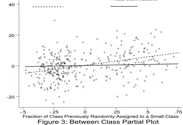
fraction of student i’s classmates who were previously in Small classes, must have sufficient variation after its linear dependence onDj is factored out. This is clearly where the degree of New Entrants, and in particular, the extent to which the New Entrants are spread across classesjis key to give the instrument any chance of power in our data. As we show in Figures 1 and 2, fortunately for our purposes, the Fraction of New Entrants does indeed have signiÞcant
variation across classes for all three grades. Figure 1 is a histogram of the fraction of each Small class who were previously randomly assigned to a Small class as well. Were there no new entrants, and no students switching class type, the histogram for each grade would be a single bar at 1. In fact, we can see while there is a pronounced tendency for that fraction to fall between 0.5 and 1, the histogram reveals substantial variability in this fraction across classes. Figure 2 does the same exercise for the Regular classes, where absent the new entrants and switchers, each histogram would be a single bar at 0. While the variation across classes here is less visually apparent, it is also clear we have some power. Finally, as we shall see below when we present theÞrst-stage regression results, this net variation (net of the Small class indicatorDj) in the instrument also has decent explanatory power at the third grade level, and moderate at the second grade level, for the peer group outcomes.
The inclusion of the class type indicator Dj also helps ease the exogeneity requirements for the group formation. For example, the presence of the class type indicator in the regression has the effect of sweeping out all observed and unobserved factors that vary purely at the class type level. So if we assume that the (possibly endogenous) sorting that takes place within class types of students and teachers into particularclassesis the same for the Small and Reg-ular classes, then the presence of theDj treatment indicator will ‘balance the bias’ (Heckman, 1997) and net it out of our estimated equation. The point is that randomization creates two groupings of students and teachers that are, in principle, identical on either side of the treatment and control line. While the sortingwithinthe two clusters of students and teachers into classes may well be endogenous, as long as that process is the same for both groups, the presence of the treatment indicator will guarantee that it will be differenced out. Of course, if students and teachers are assigned not just to classtypeson the basis of randomization, but also individual classes within class types, then this entire discussion is moot. But we have been unable to verify with certainty that all schools in the Project STAR experiment created classroom groupings via ran-domization, and so we proceed under these weaker assumptions. While the idea of identical endogenous processes leading to class formation (under the scenario where we dispense with the possibility that classes were formed via a random-ization scheme), we should mention it is not difficult to construct behavioral models in which these processes would not be identical owing precisely to the differing class sizes on either side of the treatment and control lines.15 That is a very nuanced version of the endogenous sorting story, and to speak more to it empirically would require far richer data than we have access to here.
Our instrumental variables strategy yields differences in the power to detect peer effects across grades. First, it should be obvious by the very nature of our identiÞcation strategy, in that it relies on the lagged Small class assignment 15A point we owe to Andy Foster for pushing us think beyond the purely statistical statement
variable, that peer effects will not even be estimable via this strategy for Kinder-garten. Given that not all children attend Kindergarten in Tennessee, this is perhaps not a serious shortcoming of our strategy. By default, we assign all of the reduced form effect to the ‘pure’ class size effect in examining the Kinder-garten class type estimate, although what we are really saying is that, given our identiÞcation strategy, we cannottellif some portion of this effect is really being driven by peer group effects or some other source. Similarly, while we are not prohibited from empirically estimating a peer group effect for the First grade with our strategy, as we will see, we really have quite low empirical power. This brings us to the conceptual point we wish to make on this subject in this section. Because our identiÞcation strategy literally relies upon thefeedbackof the treatment assignment effect on students as the Project STAR cohort ages, we expect to see greater notional power for the later grades. We wish to stress that of course the failure to detect an effect does not imply there isno effect, and so in our context the failure to detect peer effects in the early grades may simply be symptomatic of the very design of our identiÞcation strategy.
To summarize this section, we rely most heavily on the aspect of Project STAR that it randomly assigns a Small class treatment to individuals and then clusters those children differently as the experiment progressed across grades. This is the key to our identiÞcation strategy in extracting measurement of the endogenous peer group effects from these type of data. We will discuss the speciÞc econometric properties of our estimation scheme and how itÞts in with a more general discussion of peer group effects in Section 5 below. We do not argue that the students in Project STAR are randomly placed into individual classes, but merely class types (Small or Regular) within each participating school. The technical literature on this aspect is unclear, and in any case, our strategy is operational if, as we assume, students and teachers are only guaranteed to be assigned randomly to class types and not purely classes. The bottom line is we are relying on the social multiplier effects of the class size reductions to identify the peer effects and not the random assignment of students to different peer groups. The extra assumption we must incur lacking the random assignment to individual classes is that the potential sorting that does occur along the lines of our instrument is the same process across the two randomly determined treatment groups. Finally, as we stated at the outset, we have for now adopted the canonical approach of the literature in other respects, such as adopting the regression model that is linear in the peer group mean outcome as well as the extremely critical assumption that the relevant peer group is the student’s classmates as regards the test score outcomes.
4
The Evidence on the Social Multiplier E
ff
ects
of the Small Class Size Treatment in Project
STAR
In this section we use the Project STAR data together with our identiÞcation strategy just discussed in the previous section to estimate peer effects. Before we move to that estimation framework, weÞrst replicate the earlier work done with Project STAR on the class size effects as in Krueger (1999), and then interpret these as reduced-form (or total) class size effects that we try to pull apart into their underlying components of the peer group effect and the residual which we call the ‘pure’ class size effect. We consider both the instrumental variables as well as the reduced form results, the latter of which combine the direct class size effects together with the social multiplier or feedback effects created by the experiment. The reduced form allows us to begin to perturb the canonical framework to alternative speciÞcations. We also consider the robustness of our baseline instrumental variables results to alternative instrumentation strategies, as well as assess the sensitivity of our results to departures of the Project STAR data from the experimental protocol (such as class type switchers).
4.1
Estimates of the Peer E
ff
ects and the Pure Class Size
E
ff
ects: Inside the Black Box of Project STAR
We begin our empirical analysis withÞrst presenting the reduced-form class size effects using the Project STAR data. The results are broken out by the four grades for which the experiment ran, and as we discussed above, all regressions include school Þxed-effects as the STAR data were not a random sample of schools. Owing to the randomization of students and teachers within schools to the three class types - Small, Regular, and Regular with a teacher’s aide (we use Regular as our omitted base group) - a simple OLS regression estimates the treatment effects of interest as the coefficients on the Small and Regular/aide dummies.16 These results are presented in Table 3, and our results reproduce the
analogous results presented by Krueger (1999) and Hanushek (1999) (without regard to their subsequent interpretation of these results). In short, the Regu-lar/aide classes do marginally better, although the difference is not statistically distinguishable from the Regular class base group. The Small class estimates, however are all quite signiÞcant at conventional levels, and range from a low of 4.8 percentile points to a high of 7.3 percentile points relative to the Regular class students. It is not much violence to these results to summarize them as saying that being in a Small class appears to have roughly a 5 percentile point 16In an experimental setting, the inclusion of covariates helps in countering small
imperfec-tions in the randomization along observable dimensions, but primarily serves to reduce the residual uncertainty and so reduce the sampling error of the effects of interest.
gain over students in Regular classes (of either type) at each of the four grade levels.
What we wish to do is essentially pry apart this 5 percentile effect into its constituent components of a pure class size effect and the peer group effect which is the focus of our work. An alternative statement of our goal is to split the class size effect into its direct and indirect effects, although this language is rather imprecise and leaves the implications for policy counterfactuals rather muddled. Whereas earlier authors, especially Krueger (1999), interpreted the roughly 5 percentile point gain implied by the coefficient on the Small Class indicator as pertaining to the causal effect of the Small Classsizeas compared to the omitted control group, Regular Classes, we wish to remain more agnostic at this stage.
We interpret this as the total effect of being assigned to the Small Class
type, but we view this categorization as a bundle of components which comprise the ‘black box’ of the class type, and which may include peer effects and other elements of a general schooling production function. At the inception of the program (i.e. Kindergarten and possibly First Grade) it seems plausible that the cohort design to the study would more precisely reßect a pure class size effect. But as the cohort ages, it becomes increasingly difficult to argue that the simple contrast between the Treatment and Control groups reßects a pure class size effect, without allowing for the possibility that the experimentally induced changes in the peer group compositions might also play a role. What the earlier literature as exempliÞed by Krueger (1999) and Hanushek (1999) focused on was the lack of widening of the gap between the students who remain in the Small classes as the experiment progressed, and why the 5 point gain appeared to be a once and for all gain, as opposed to an increase in the slope of the test score-grade relationship as well as in the intercept.
Table 4 presents the simplest possible departure from the Treatment and Control indicators used to measure the class size effects from Table 3. In Table 4 we include the additional characteristic of the classes given by the average (leave-out mean) test score of the class ¯y−i,j - a measure we intend to capture the ‘peer group effects’ as articulated in Section 3 above. We are not trying to ascribe any behavioral signiÞcance to these regressions, but we want to present a benchmark by which the IV estimates we present below might be compared. In particular, owing to the reßection problem which we discussed in Section 2, the individual outcomeyijand the peer group outcome ¯y−i,jare simultaneously determined and so the reverse causality would have to be considered formally to give this a behavioral interpretation.17 The remarkable stability of the es-17As we discussed in Sections 2 and 3, we do not have test score outcomes for the New
Entrants prior to their entry to the Project STAR schools. Therefore, we cannot resort to
ad hocÞxes to the reßection problem by utilizing a lagged version of the peer group measure (i.e. the student’s current peers’ test score in the previousgrade). However, we did use, purely for comparison sake, the lagged mean peer group effect lagged one grade for those students who were in the Project STAR schools in the previous grade. This exercise has
timated coefficients across grades on the peer effect measure certainly presage the analytical results we consider in the next section and in the Appendix that derive the sample properties of the type of peer group estimators considered in Table 4. Across the three columns, we see that the estimated coefficients on the peer group measures are virtually identical at 0.58 with standard errors of 0.04. The coefficients on the Small class indicators exhibit a little more heterogeneity across grades, and they have fallen to roughly half their original magnitudes from the total program effect estimates given in Table 3. The point estimates suggest a small decline in the Small class effects across the three grades (as in Table 3), although the decline is not statistically signiÞcant. All three esti-mates of the Small class effect, however, remain statistically distinct from zero even after including the contemporaneous peer effect measure as an additional regressor.18
At the bottom of Table 4 we present what we call the normalized peer effect which places the estimated coefficient on the peer group measure given in the Þrst row of each column on the same scale as the coefficient on the Small class indicator. Conceptually, it captures the discrete effect of moving from a Small to a Regular sized class on the average peer group measure. From a measurement perspective, we can view the sum of the effects on the Small class indicator and on this ‘normalized’ peer group effect as roughly splitting the overall (roughly 5 percentile point) reduced-form experimental effect into its constituent components of the direct class size effect and the feedback effect induced by the peer group effect. As we can see in the last row, the normalized peer effects reßect the homogeneity of the peer effect coefficients and they vary from roughly 4 to 3 points. If we sum the Small class effect in the second row of Table 4 with the normalized peer effect, we get the estimatedtotalSmall class effects of 6.66 for First grade, 5.26 for Second grade, and 4.95 for Third grade.
the effect of replacing the reßection problem which hinders the behavioral interpretation of the results in Table 4 with another problem, which is, what does the lagged peer group measure mean if it is only constructed over those students who were in the experiment last year? Interpretation problems aside, we Þnd the biggest change occurs in theÞrst grade, where the estimated coefficient on the peer effect drops from the estimated 0.58 in Table 4 to 0.05 with a standard error of 0.07. The second and third grade estimates on the peer group measure drop by about half to 0.21 for both grades. For the most part, the Small class dummy coefficients remain qualitatively the same, although the point estimates show a more pronounced monotonic decline across grades. But as both versions of Table 4 suffer from measurement or simultaneity problems, we only use them to serve as a benchmark to contrast our later results to.
18Here again we would be remiss if we did not point out the presence of the reßection problem
and the problems with interpreting the results in Table 4 behaviorally. As regards the Small class effect, obviously one potential impact is that it enhances the performance of a student’s peers. Therefore, including it as a covariate will obviously diminish the potential effect of the Class size mechanism, as it simply splits the total effect displayed in Table 3 into a direct and indirect effect, with the contemporaneous peer group measure being a potential outcome of thecontemporaneousclass type indicator. The IV estimators considered below do not have this mechanical problem of simply splitting the overall effect of purely the contemporaneous class size measure.
If we compare these to the total experimental effects of the Small class type presented in Table 3, these were 7.31, 5.94, and 4.76. Thus, for the most part, the Small class direct effect and the normalized peer effect combined appear to account for the average total experimental effect of the Small class assignment. We turn now to our instrumental variables strategy which avoids the reß ec-tion problem and also accounts for the aspect of the sampling design of the experiment in that we do not have test scores for the New Entrants prior to their joining the Project STAR schools. As we discussed in the previous sec-tion, we use as an instrument for the contemporaneous peer group measure ¯y−i,j the fraction of the current peer group students who were assigned to the Small class treatment in the previous grade z−i,j ≡ N1−1PNk6=idkj. The instrument therefore treats students who are either New Entrants to the experiment or pre-viously randomly assigned to one of the Regular class types as the same as far as explaining variation in the class to class variation in average test scores.19
As we noted in our conceptual discussion in the previous section, this strat-egy looks to have promise since the fraction of students who were previously randomly assigned to a Small class has good variation across classes for the Small class type group (owing to the signiÞcant quantity of the New Entrants). In Table 5 we present the Þrst stage of the projection of ¯y−i,j on z−i,j. We
do this by grade, and as the grade increases, obviously the number of potential instruments grows, as students may haveÞrst been exposed to the Small class treatment in an ever-increasing number of prior grades. So, for example, by the third grade, there are three such possible instruments. By looking at the Þrst three rows of Table 5, the reader can see that for the most part, the instruments are individually generally not statistically distinct from zero. The exceptions to this are the Kindergarten effect for the Second grade regression, which is marginally statistically signiÞcant, and the rather large point estimate for the Third grade, which is highly signiÞcant at conventional levels. The joint test on the combined signiÞcance of the instruments for each regression is given in the 4th row from the bottom of the table. There the reader can see we have quite low power for the First grade, weak to moderate power for the Second grade, and quite good power for the Third grade owing largely to the Kindergarten peer measure effect. This pattern of power for our instrumental variables framework we anticipated in our previous conceptual discussion of our strategy, as it relies directly on the feedback notion of what a peer group effect is, and so it only be-comes detectable as the cohort ages and the feedback effects potentially surface from the environment.
19To the extent that the ‘Regular’ class size represents the average class size in the schools
from which these students came, this may not be such a bad approximation. The random assignment of the New Entrants to the Small and Regular class types helps balance the differences between the New Entrants and the previously assigned students along unobserved dimensions once the contemporaneous class type indicatorDjis conditioned on. As we noted
in Section 2, however, there is plenty of evidence to suggest thatunconditionally the New Entrants and those students previously randomly assigned to even just Regular classes are
Notice also that because we are instrumenting for a grouped version of the dependent variable, theÞrst-stage regression is also almost the reduced form for the two equation system at the individual level.20 Therefore, we can also exam-ine the effect of the class type indicators after holding constant the direct peer treatment effects of interest. This approach has the advantage of avoiding any sort of reßection type problems. However, as regards our principle identifying assumption, it may be subject to the endogenous sorting objection if the sorting is systematically different between the Small and Regular classes. But keeping with our assumption that this bias is balanced across the treatment arms of the experiment, then the coefficients on the Small class indicators tells us to what extent the Small class effect of Table 3 is only reßective of the spillover effects generated by the past impact of the experiment. Indeed, while the Small class effect for the First grade, 6.39 (and statistically distinct from zero), is still close to its Table 3 estimate, the point estimate for the Grade 2 effect is half its Table 3 value, and is statistically indistinguishable from zero. Finally, the Grade three point estimate is actually negative, but is again indistinguishable from zero. Thus, our conclusions which we shall discuss below regarding the insigniÞcance of the Small class effects at Grade 2 and 3 of the Project STAR experiment are not subject to a criticism that we may have mishandled the treatment of the endogenous peer effects. Once measures capturing the prior exposure to the Small class treatment of an individual’s peers are included, the current effects of having been assigned to a Small class are substantially attenuated.
The second stage instrumental variables results presented in Table 6 rep-resent the core results of our paper. They show that once we account for the simultaneous determination of the individual yij and contemporaneous peer group outcomes ¯y−i,jusing the lagged fraction of the peer group exposed to the treatment as an instrument, the estimated peer effects swamp the direct Small class size effects in grades 2 and 3. The Þrst grade point estimate of the peer effect is roughly one-third of the second and third grade estimates, and is quite imprecisely estimated. As such, it is indistinguishable from no effect, although as we indicated above, and we wish to stress again, this lack ofÞnding an effect should certainly not be construed to imply that there is no effect, as the power of the empirical design is quite weak here. Indeed, the conÞdence interval on the
Þrst grade effect more than encompasses the Second and Third grade effects, and so could even be construed as consistent with those point estimates.
20The use of the term ‘almost’ here may be unclear. For the most part, the dependent
variable in theÞrst stage regression presented in Table 5, ¯y−i,j varies little across students
within classes, but more so across classes. Below we shall consider reduced forms purely at the classroom level, as the treatments of interest vary only at the class level rather than the individual level, and so in this sense, the standard errors presented in Table 5 over-count the degrees of freedom for these treatments. The class level results are presented in Appendix Table 1, and show that our correction for the within-class correlation of the errors almost completely compensates for the possible overstatement of the degrees of freedom. Thus, inferences drawn from Table 5 are not deceptive owing to the ‘over-counting’ of the degrees of freedom.
The normalized peer effects are presented in the last row of Table 6, and roughly speaking, the Second and Third grade effects have a point estimate of about 4.5. The Small class effects presented in the second row are now extremely small relative to the 5 percentile point estimates of the overall effect presented in Table 3, and quite indistinguishable from zero. Given the precision of the standard errors on these two point estimates, we can clearly reject their equality to the earlier reduced-form effects. This pattern is reversed, however, for the First grade estimates. There the Small class effect remains largely unchanged at 4.91, although the standard error on this estimate is extremely large, so it is also indistinguishable from zero. The estimated normalized peer effect is less than half the grade two and three effects, at roughly 2 percentile points. The associated t-statistic, however, is less than 0.30, reßecting the low power, and as we already noted, the peer effect for the First grade is indistinguishable from 0.
This very stark pattern of the apparent complete overtaking of the Small class size effect by the peer effect as of the second grade may strike the reader as unusual, and perhaps indicative of some spurious attribute of the setting driving these results. For that reason we next turn to examining the sensitivity of these basic results to alternative speciÞcations and measurement schemes. However, it is also useful to pause for a moment and point out one exercise this paper will not be able to shed much light on. Namely, as a measurement device, we have posited that individual outcomes vary with the mean outcomes of the reference group. But we have not considered the behavioral model by which these individual outcomes, which are presumably the result of underlying choices and inputs, come to be inßuenced by the reference group. Manski (2000) among others has delineated three broad channels by which the peer group mechanism might propagate: 1. Preference interactions 2. Expectation interactions and 3. Constraint interactions. While we certainly agree that for the evidence in this paper to lead to precise policy prescriptions we would need to establish how these behavioral mechanisms lead to the peer group inßuences we observe, we emphasize that the Project STAR data do not sample characteristics that enable us to speak to these alternative explanations empirically. It is possible at this juncture to offer stories which might rationalize this pattern of results across grades that rely differently on say the preference versus the expectations rationales behind the peer inßuences, but we shall avoid thisex posttheorizing in this paper, and leave this exploration until the relevant variables can be sampled.
4.2
Assessing the Robustness of the Peer E
ff
ect Results
Table 7 presents our Þrst set of robustness checks of our basic speciÞcation presented in Table 6. Essentially this table is concerned with the fact that since each student in Project STAR can be represented as a given experimentally assigned ‘type’, then using one source of variation is equivalent to using one
minus another source of variation. For example, each student currently in a Small class was either previously randomly assigned to a Small class last year (PRASC), a New Entrant to the Project STAR schools (NE), or one of the rather small fraction of class type Switchers (S). If we let each of these variables denote their respective fractions, then we have for each Small class:
1 =P RASC+N E+S (5) So then it is identically true that for just the Small classes, using the fraction PRASC as an instrument, as we did in Table 6, is equivalent to using (1 NE -S) as an instrument.
For the Regular type classes, a student who was PRASC who is now in a Regular class is clearly a Switcher, and so we will replace the designation of switcher to PRASC for the Regular classes, to keep the notation for a Switcher, S, as beingjustfor those who switch from a Regular to a Small class. Introducing the notation of PRARC for those students who are in a Regular class now who were previously randomly assigned there, we have:
1 =P RARC+N E+P RASC (6) So now we have the identity that PRASC = 1 - NE - PRARC, and so using PRASC as an instrument for the Regular classes is identical to using 1 NE -PRARC as an instrument. Notice we have purposefully not used notation to distinguish between New Entrants to Regular classes versus New Entrants to Small classes, as the randomization should equate those two groups. However, PRARC and PRASC are potentially distinct groups as they have been exposed to different treatments at an earlier point in the experiment.
The basic point of spelling out these identities is that using the variation explained by the proportions of students in the classes who were, for example, previously randomly assigned to a Small class is identically the same as using the ‘mirror image’ (and thus the same Þrst stage projection and the same IV estimate) proportions of the other groups of students across classes. This point is useful to keep in mind in interpreting Table 7. First, we can examine the possibility that the peer effect works differently for the Small and Regular class types. Therefore, the Þrst row of Table 7 pools the class types as in Table 6 and uses PRASC as the instrument, thus replicating the Þrst row of Table 6. The next two rows allow the peer effect to be potentially different across class types. For the Third grade, the estimated peer effect coefficients are roughly the same, and roughly average to the pooled Third grade effect presented in Table 6. For the Second grade, the Small class peer effect is roughly the same as the pooled Second grade effect from Table 6. However, when looking just within the Regular classes, the estimated peer effect is highly imprecise and the point estimate is actually negative. Now here is where the identities just presented become useful. As we noted above, for the Regular classes, the number of students PRASC is equal to the number of Switchers (into Regular class types).
Therefore, a regression which uses only the fraction of class type Switchers will produce an identical point estimate, and by looking at the last row of Table 7, the reader can see that the -0.56 point estimate from the third row is identical to the -0.56 estimate for the Second grade in the last row.
Thus, when we allow the peer effect coefficient to differ by class type, we can see that in the case of the Second grade, the point estimate is quite different for the Regular classes than for the pooled (across class types) estimate given in Table 6. Likewise for the peer group effect for the Regular classes for the First grade as is shown in the Þrst column of the third row of Table 7. In contrast to the Table 6 pooled estimate, the point estimate here is roughly the same magnitude (and statistical signiÞcance) of the Second and Third grade estimates from Table 6. And of course here again, the estimate is identical to the First grade estimate for the Regular classes in the last row of Table 7 which uses the fraction of class type Switchers as the excluded instrument. Our point in displaying this numerical equality of the estimated effects, as well as the brief conceptual discussion we just provided on the ‘reverse image’ form of identiÞcation is precisely to highlight to a skeptical reader that our identiÞcation strategy uses different groups to identify effects when we pool across class types. The reader, for possibly good reasons, may be worried about relyingentirelyon class type switchers to identify a peer group effect, as students who opt to switch class types (in this case the somewhat more unusual choice of switching from a Small to a Regular sized class) is endogenously determined with respect to the outcome. Such readers may therefore wish to discard those aspects of our analysis that include these Switchers as a source of identifying information. For this reason, they may wish to instead focus on the Small class estimates given in the second row of Table 7, as opposed to the pooled class type estimates given in Table 6.
The Small class peer effect estimates from the second row of Table 7 are qualitatively the same as the pooled peer effect estimates from Table 6 for the Second and Third grades. The First grade peer effect estimate, while still quite imprecisely estimated, is now quite large at 1.72 and is statistically distinct from zero at conventional levels. This discrepancy with our Table 6 results is in some sense reßective of the low power properties of our identiÞcation design with regards to the First grade setting that we have discussed previously. Across the multiplicity of speciÞcations we have presented both in the paper, as well as those not presented, we tend toÞnd much more systematic and uniform peer effect estimates for the Second and Third grade, whereas the results for the First grade are much more mixed and far more speciÞcation dependent.
This pattern is also seen in the speciÞcations we present in the middle rows of Table 7 where we now use the percent of New Entrants in the class as the instrument for the peer group measure. The idea here is to use the variation in peer group ‘quality’ induced by those students who werenotexposed to either the treatment or control groups of Project STAR. As we noted in discussing our primary identiÞcation strategy underlying Table 6, we might expect that the
New Entrants are comparable to the students already assigned to the control classes in the Project STAR groups, but if there is some type of spillover, or simply that the New Entrants represent a distinct group apart from the pre-existing Project STAR students, then this strategy might be appropriate. Our primary intent, however, is not to offer a strong behavioral justiÞcation for this instrumental variables strategy, but simply an alternative measurement strat-egy of the peer group coefficient. For the most part, our conclusions from the other parts of Tables 6 and 7 stand. The Second and Third grade results tend to be statistically distinct from 0, although the estimated effects are diminished in comparison to Table 6. This is especially true when we break the estimated effects out by class type and we look at the effects for just the Regular classes - these effects are roughly half of their Table 6 counterparts. Part of this at-tenuation might arise from the mixing of the students previously assigned to
eitherSmall or Regular classes under this identiÞcation strategy. For the First grade, we doÞnd a statistically and economically signiÞcant estimated effect for the pooled class type speciÞcation, but the effect estimated for just the Small class types is highly imprecise, and fo