UNIVERSIDAD DE VIGO
DEPARTAMENTO DE FÍSICA APLICADA
Environmental Physics Laboratory
PhD Thesis
DualSPHysics: Towards High Performance Computing
using SPH technique
Memoria Presentada por José Manuel Domínguez Alonso para obtar al título de DOCTOR POR LA UNIVERSIDAD DE VIGO CON MENCIÓN INTERNACIONAL Septiembre, 2014
Informe del director
Dr. Alejandro Jacobo Cabrera Crespo, Contratado Juan de la Cierva de la Universidad de Vigo, y Dr. Ramón Gómez Gesteira, Catedrático del Departamento de Física Aplicada de la Universidad de Vigo:
CERTIFICAN
Que la presente memoria “DualSPHysics: Towards High Performance Computing using SPH technique”, resume el trabajo de investigación realizado,
bajo su dirección, por DON JOSÉ MANUEL DOMÍNGUEZ ALONSO en el departamento de Física Aplicada en el programa de doctorado de Ciencias del Clima: Meteorología, Oceanografía Física y Cambio Climático de la Facultad de Ciencias de Ourense para optar al título de “DOCTOR POR LA UNIVERSIDAD DE VIGO CON MENCIÓN INTERNACIONAL”.
Y para que conste y en cumplimiento de la legislación vigente, firman el presente informe en Ourense, a 23 de Septiembre del 2014.
Fdo: Dr. Alejandro Jacobo Fdo. Dr. Ramón Gómez Gesteira Cabrera Crespo
Acknowledgements / Agradecimientos
En primer lugar me gustaría mostrar mi agradecimiento a Moncho por abrirme las puertas del apasionante mundo de la investigación, por su confianza y su tiempo. A él le debo gran parte de las nuevas experiencias vividas estos años, los lugares que he visitado, las cosas que he aprendido. Aunque también las noches sin dormir tratando de ir siempre un poco más allá.
A Alex, mi director, compañero y amigo. Gracias por su ayuda inestimable y todo su tiempo, tanto en el trabajo como fuera. Sin él, gran parte de lo conseguido no hubiera sido posible.
A todos mis compañeros de ahora y antes: Anxo, Orlando, Fran, Xurxo, Isabel y Alex, que siempre logran hacer del trabajo un lugar ameno. Sin olvidar a toda la gente del laboratorio.
To people in Manchester: Ben, Georgios, Athanasios and Abouzied, for their hospitality and help when I was away from home.
A mis amigos de Orense: Diego, Noe, Sandra, Noelia, Victor, Dani, Carlos, Edu y Marta, por estar siempre ahí y hacer imposible que me sintiese solo en esta ciudad.
A mis amigos de siempre: David, Hugo, Eva, Txatxo, Arancha, Nuria, Borja, Vero, Alberto, Mar, Dosy, Lucy, Dulci, Juan, Fernando, Ester y Toni, por los innumerables días y noches que he disfrutado de su compañía.
A Patricia por su cariño, su apoyo, su paciencia… por aguantarme que Dios sabe que no es fácil.
Muy en especial a mi madre, mi padre y mi hermana, que sin ellos no sería nada. Por ese amor incondicional que por mucho que lo intente, nunca podré devolverles en la misma medida en que lo recibo.
This work was partially supported by Xunta de Galicia under Axudas de apoio á etapa predoutoral do Plan Galego de Investigación, Innovación e Crecemento 2011-2015, Axudas a grupos de investigación do Campus de Ourense (INOU2013), project Programa de Consolidación e Estructuración de Unidades de Investigación Competitivas (Grupos de Referencia Competitiva), funded by European Regional Development Fund (FEDER) and Ministerio de Economía y Competitividad under project BIA2012-38676-C03-03.
Resumen
El objetivo de esta tesis es la investigación usando técnicas de programación de alto rendimiento aplicadas al modelo numérico Smoothed Particle Hydrodynamics (SPH) y su uso para llevar a cabo el desarrollo de una aplicación informática capaz de realizar simulaciones de casos reales con SPH en un tiempo de cálculo razonable.
La estructura de este trabajo se describe a continuación:
El capítulo 1 introduce conceptos básicos sobre la simulación numérica. Se describen las principales características del método SPH. Se muestran algunas ideas generales de HPC. Se introduce el código DualSPHysics asociado a esta tesis.
El capítulo 2 proporciona los fundamentos teóricos y conceptos básicos del modelo SPH tales como el método de interpolandos, los kernels de suavizado, las ecuaciones físicas involucradas, los algoritmos de paso de tiempo y el tratamiento de las condiciones de frontera.
El capítulo 3 describe los pasos principales de la simulación de un código SPH y su implementación en DualSPHysics. Concretamente se centra en la creación de la lista de vecinos. Este capítulo se basa en el artículo científico [Domínguez et al., 2011a].
El capítulo 4 trata diferentes estrategias para mejorar el rendimiento de DualSPHysics en CPU (Unidad Central de Procesamiento). Se presenta una implementación con OpenMP y se muestran los resultados de mejora obtenidos. Este capítulo se basa en el artículo científico [Domínguez et al., 2013a].
El capítulo 5 trata las diferentes estrategias de optimización aplicadas a DualSPHysics en GPU (Unidad de Procesamiento Gráfico) utilizando CUDA. Se tratan no sólo las técnicas de optimización básicas descritas en los manuales de CUDA, sino también otras optimizaciones de GPU intrínsecas al método SPH. También se muestra su impacto y la eficiencia alcanzada en diferentes arquitecturas de GPU. El rendimiento del código GPU también se compara con el de CPU multi-core. Este capítulo se basa en los artículos científicos [Crespo et al., 2011] y [Domínguez et al., 2013a].
haciendo posible la ejecución de SPH en clústeres heterogéneos. En concreto, la implementación propuesta permite la comunicación y la coordinación entre múltiples CPUs, que también pueden albergar GPUs, permitiendo ejecuciones multi-GPU del método SPH. Este capítulo se basa en el artículo científico [Domínguez et al., 2013b].
El capítulo 7 aborda la cuestión de precisión en el cálculo numérico y aplica soluciones al problema de falta de precisión que surge en algunos casos. Se estudia el uso de doble precisión en GPU de forma que la pérdida de rendimiento sea mínima. Este capítulo se basa en la publicación de congreso [Domínguez et al., 2014].
El capítulo 8 presenta las conclusiones de esta tesis, junto con el trabajo propuesto para un futuro próximo, además de mencionar el que ya está en desarrollo.
El apéndice A contiene la documentación de DualSPHysics con un resumen de los archivos de código fuente, cómo compilar y ejecutar el código y la descripción de los archivos de entrada y de salida, así como su formato. Este apéndice se basa en el artículo científico [Crespo et al., 2014].
El apéndice B describe la herramienta de pre-procesado implementada para crear la configuración y condición inicial de simulación usada por DualSPHysics. Este apéndice se basa en la publicación de congreso [Domínguez et al., 2011b].
El apéndice C describe las herramientas de post-procesado que permiten realizar un análisis numérico de los resultados, así como visualizar la simulación resultante.
La naturaleza puede ser modelada buscando las soluciones analíticas de las ecuaciones que definen un sistema (o modelo numérico). Una vez que las ecuaciones son validadas, el comportamiento del sistema puede predecirse ajustando algunos parámetros e imponiendo un conjunto de condiciones iniciales. El modelado numérico busca resolver estas ecuaciones de un modo numérico en lugar de analítico. De esta forma, diseñando algoritmos que hacen uso de números y reglas matemáticas simples se pueden simular procesos complejos del mundo real. La simulación numérica es una potente herramienta que permite comprender el comportamiento de sistemas complejos e incluso predecir su evolución a partir de unas condiciones iniciales. El modelado numérico adquiere mayor importancia con la llegada de las computadoras, ya que estas máquinas
operaciones matemáticas sencillas.
La Dinámica de Fluidos Computacional (CFD) es una rama de la mecánica de fluidos que estudia su comportamiento mediante el uso de modelos numéricos. La principal ventaja de esta técnica es su capacidad para simular escenarios complejos y proporcionar datos físicos que pueden ser difíciles, o incluso imposibles, de medir en un modelo real. A pesar de la exactitud de los modelos numéricos, estos no pueden sustituir a la construcción de modelos a escala, pero sí pueden reducir significativamente el número de pruebas físicas. Esto último da lugar a un ahorro importante en tiempo y dinero, ya que la construcción de modelos físicos es muy cara y lenta.
Hay dos aproximaciones numéricas para describir el movimiento del fluido; Euleriana y Lagrangiana. El enfoque Euleriano resuelve las ecuaciones en los nodos fijos de una malla. Mientras que en la descripción Lagrangiana del fluido, las posiciones donde las ecuaciones son resueltas, también se mueven con el fluido sin necesidad de usar una malla fija. Los métodos basados en el uso de una malla (elementos finitos, diferencias finitas y volúmenes finitos) son actualmente robustos, maduros y se han aplicado a una amplia gama de aplicaciones proporcionando resultados muy precisos. Estos métodos basados en malla son ideales para sistemas en los que el dominio está perfectamente definido y para simulaciones donde los límites se mantienen fijos. Sin embargo, la creación de la malla puede ser muy ineficiente si el sistema es complejo. En los últimos años, numerosos métodos sin malla han aparecido y crecido en popularidad, ya que se pueden aplicar a problemas que son altamente no lineales con geometrías complejas y difíciles para los métodos basados en malla. Dentro de los métodos sin malla ahora disponibles, Smoothed Particle Hydrodynamics (SPH) es, probablemente, el más popular y ha alcanzado el nivel necesario de madurez para ser utilizado para propósitos de ingeniería.
SPH es un método sin malla Lagrangiano que se utiliza cada vez más para una amplia gama de aplicaciones dentro del campo de la Dinámica de Fluidos Computacional. Inventado originalmente para la astrofísica en los años setenta [Lucy, 1977; Gingold and Monaghan, 1977], se ha aplicado en muchos campos diferentes, incluyendo la dinámica de fluidos y la mecánica de sólidos. El método utiliza partículas para representar un fluido y estas partículas se mueven de acuerdo a la dinámica que rige. Al simular los flujos de superficie libre, no es necesario un tratamiento especial de la superficie debido a la naturaleza
SPH se ha utilizado para describir una gran variedad de flujos de superficie libre (propagación de olas en una playa, impacto sobre las estructuras y roturas de presas). El primer intento de estudiar los flujos de superficie libre fue presentado por [Monaghan, 1994]. Monaghan también estudió el comportamiento de corrientes de gravedad ([Monaghan, 1996]), ondas solitarias ([Monaghan et al., 1999]) y la llegada de olas a la playa ([Monaghan and Kos, 1999]). Más tarde, el modelo se aplicó al estudio de la interacción de olas con estructuras en [Colagrossi and Landrini, 2003]. El problema clásico de rotura de presas también se estudió en 3D por [Gómez-Gesteira and Dalrymple, 2004]. Dentro del área de la ingeniería costera, SPH fue empleado para estudiar la interacción de las olas con un rompeolas en [Gotoh et al., 2004] y [Shao, 2005].
Sin embargo, el elevado coste computacional de este método constituye un inconveniente importante. Simular un período de tiempo físico reducido requiere un elevado tiempo de ejecución cuando se ejecuta en una única Unidad Central de Procesamiento (CPU). Esto es debido a la gran cantidad de interacciones entre partículas que se tienen que calcular en cada paso de tiempo. Este problema ha obstaculizado el desarrollo de SPH y su uso industrial para resolver problemas reales. Por ello, la capacidad de realizar cálculos que impliquen millones de partículas en un tiempo razonable es esencial para llevar a cabo simulaciones relevantes en la industria. Sin embargo, esto sólo es posible si se emplean algunas técnicas de Computación de Alto Rendimiento.
La Computación de Alto Rendimiento (HPC) es un campo muy dinámico que se ocupa del estudio y el uso de nuevos recursos y nuevas tecnologías computacionales. Su objetivo es resolver problemas muy complejos que requieren una gran capacidad de cálculo, de manera que no se pueden resolver con los sistemas informáticos convencionales, lo cual hace necesario el uso de clústeres o supercomputadoras.
Un supercomputador es un computador con una elevada velocidad de cálculo dedicado a la ejecución de operaciones en paralelo y diseñado para la computación intensiva. Se trata de máquinas muy caras. Por otro lado, un clúster es un conjunto de ordenadores conectados a través de una red de alta velocidad que se tratan como una sola máquina. Esta es una opción más económica, ya que puede estar formado por máquinas convencionales, que actualmente tienen un alto rendimiento a precios muy bajos. Los clústeres también ofrecen la
HPC incluye múltiples técnicas de computación paralela y computación distribuida. En general, la computación paralela consiste en la ejecución de varias operaciones simultáneamente.
La computación paralela se puede aplicar en máquinas de memoria compartida. En cuyo caso la máquina tiene uno o más procesadores que utilizan el mismo espacio de memoria. Las herramientas de programación más extendidas para este tipo de arquitectura son pthreads [Buttlar et al., 1996] y OpenMP [Chandra et al., 1996; Chandra et al., 2002]. OpenMP se puede considerar como el estándar para sistemas de memoria compartida debido a las ventajas que ofrece sobre otros modelos de programación paralela [Dagum and Menon, 1998]. La computación paralela también se puede aplicar en sistemas de memoria distribuida, en los cuales cada procesador tiene asociado un espacio de memoria y no se puede acceder directamente a la memoria de otros procesadores. En este tipo de arquitectura, el intercambio de datos entre los procesadores debe llevarse a cabo de forma explícita utilizando un modelo de paso de mensajes. Las opciones más comunes para este tipo de programación son PVM [Geist et al., 1994], BSP [Bisseling, 2004] y MPI [Pacheco, 1996; Snir et al., 1998; Gropp et al., 1999] que es el estándar actual.
También es importante comentar que en los últimos años, el uso de procesadores de propósito especial como sistemas paralelos de propósito general se está volviendo cada vez más importante en el entorno de HPC. Actualmente, procesadores de propósito especial tales como Unidades de Procesamiento Gráfico (GPU), Procesadores Digitales de Señal (DSP) y Field Programmable Gate Array (FPGA) son utilizados como sistemas de computación científica.
A continuación se explica con más detalle las principales técnicas de HPC utilizadas para acelerar el SPH en este trabajo.
OpenMP (Open Multi-Processing) es un modelo de programación paralela para sistemas de memoria compartida. Proporciona una interfaz de aplicación de programa (API) en C, C ++ y Fortran. OpenMP es una interfaz de programación portable y flexible basado en el uso de directivas. Por lo cual su implementación no implica grandes cambios en el código. OpenMP crea múltiples hilos de ejecución que se distribuyen entre todos los núcleos de la CPU compartiendo la memoria. Por tanto, no es necesario duplicar los datos o transferir información
MPI (Message Passing Interface) es una especificación de una librería de paso de mensajes para computadores paralelos y clústeres, donde se usa una arquitectura de memoria distribuida. MPI define la especificación de una librería de funciones que se pueden llamar desde programas en C, C++ y Fortran. En este modelo de programación, una ejecución consta de uno o varios procesos que se comunican entre sí, llamando a rutinas de una biblioteca para recibir y enviar mensajes. MPI se suele combinar con OpenMP. Así, dentro de cada máquina los procesadores acceden directamente a la memoria compartida y se utiliza MPI para intercambiar información entre procesos alojados en distintas maquinas.
GPGPU (General-Purpose Computing on Graphics Processing Units) Consiste en el estudio y uso de la capacidad de cómputo paralelo de una GPU para ejecutar programas de propósito general. Las Unidades de Procesamiento Gráfico son potentes procesadores paralelos diseñados originariamente para la representación de gráficos. Sin embargo, su potencia de cálculo se incrementó mucho más rápido que la de las CPUs debido al empuje del mercado de los videojuegos (ver Figura 1). Por ello, las GPUs se pueden utilizar en aplicaciones científicas, logrando mejoras de rendimiento con respecto al uso de CPUs convencionales de 100x o más. Esto unido a su reducido precio y que pueden ser usadas en un ordenador personal, motivó que GPGPU se volviese muy popular en los últimos años [Owens et al., 2007, Nickolls and Dally, 2010]. De hecho, están surgiendo nuevos centros de supercomputación basados en GPUs impulsados por su elevada potencia de cálculo y su consumo de energía por FLOP (Operaciones de Coma Floatante por Segundo) relativamente bajo [McInstosh-Smith et al., 2012]. Tanto es así que actualmente el segundo puesto en la lista de TOP500 de supercomputadores del mundo presentado en junio del año 2014 [http://www.top500.org/lists/2014/06] está ocupado por Titan, un sistema Cray XK7 que tiene 560.640 procesadores, incluyendo 18.688 GPUs Nvidia K20x.
Las GPUs son un hardware optimizado para la ejecución paralela de operaciones de coma flotante, pero es importante mencionar que no todas las aplicaciones son adecuadas para ser ejecutadas en GPU. Realmente, sólo aquellas que exhiben un elevado grado de paralelismo. Además, deben tenerse muy en cuenta las características de la arquitectura de la GPU para obtener el máximo rendimiento. Mientras que las CPUs, diseñadas para aplicaciones de propósito general, proporcionan un acceso aleatorio a la memoria más eficiente, las GPUs
adecuados para hacer un uso eficiente de los recursos computacionales que ofrecen las GPUs.
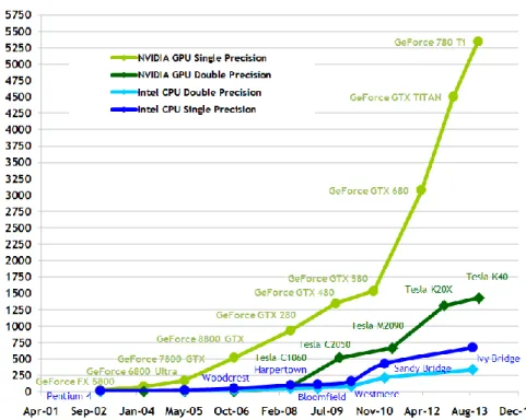
Figura 1. Rendimiento en operaciones en coma floante por segundo de CPUs y GPUs (fuente: CUDA Programming Guide v6.5).
Gran parte del éxito de GPGPU reside en la aparición de lenguajes de programación de propósito general y APIs como Brook y CUDA, ya que proporcionan un acceso más fácil a la potencia de cálculo de estos dispositivos. Brook era un compilador y un lenguaje desarrollado para las GPUs de ATI Technologies. CUDA (Compute Unified Device Architecture) es tanto un entorno de programación como un lenguaje de computación paralela específico para GPUs de Nvidia [Nickolls et al., 2008; CUDA Programing Guide]. Actualmente CUDA es el modelo de programación de GPUs más popular debido a la gran cantidad documentación y utilidades que pueden encontrarse en la web de CUDA (https://developer.nvidia.com/cuda-zone).
Por tanto, SPH es una técnica ideal para simular flujos de superficie libre. En particular, colisiones violentas entre agua y estructuras. Aunque su rango de aplicación es muy extenso, incluyendo problemas de inundaciones, diseño de defensas costeras, de embalses, de dispositivos de energías renovables… Actualmente, esta técnica se puede utilizar para propósitos de ingeniería que involucren la interacción entre agua y estructuras. En general, todos estos
necesidades computacionales. Esta es la razón por la cual es preciso optimizar y acelerar los códigos SPH.
El mayor logro de este trabajo es el desarrollo de una versión optimizada del código DualSPHysics (http://dual.sphysics.org/), código open-source que se puede usar tango en CPUs como en GPUs. DualSPHysics se ha diseñado para ser ejecutado en CPUs multi-core, las cuales son un recurso relativamente común, pero también en GPUs. La tecnología GPU ha experimentado un vertiginoso desarrollo durante los últimos años y constituye una alternativa veloz y económica a la computación clásica en CPU. No obstante, una única GPU no es suficiente para ejecutar simulaciones con grandes dominios debido a la memoria requerida. Por tanto, también se implementó una versión multi-GPU del código DualSPHysics. Además, se han desarrollado numerosas herramientas de pre-procesado y post-pre-procesado para sacar partido a las capacidades de DualSPHysics.
Las principales conclusiones de esta investigación se resumen en los siguientes puntos:
a) Lista de vecinos.
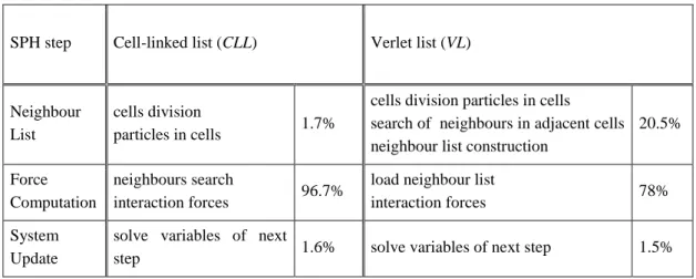
La implementación del método SPH puede dividirse en tres pasos principales; (i) generación de una lista de vecinos, (ii) cálculo de fuerzas entre partículas mediante la resolución de las ecuaciones del momento y continuidad e (iii) integración en el tiempo para actualizar todas las propiedades físicas de las partículas en el sistema. Por lo tanto, ejecutar una simulación consiste en la ejecución de estos tres pasos de forma iterativa. El paso dedicado al cómputo de fuerzas consume más del 90% del tiempo total de ejecución de una simulación, por lo que es la parte cuya aceleración es más necesaria. Sin embargo, su implementación y rendimiento depende en gran medida del paso previo (generación de la lista de vecinos). Por esta razón se lleva a cabo un estudio sobre diferentes aproximaciones para la generación de la lista de vecinos. Se comparó el uso de la lista Cell-linked y de la lista de Verlet con algunas variaciones, siendo la lista Cell-linked la elegida para ser implementada ya que proporciona el mejor equilibrio entre rendimiento y consumo de memoria.
b) Aceleración CPU.
Se implementaron cuatro optimizaciones para el código CPU de DualSPHysics. La primera consiste en aplicar la simetría en el cálculo de fuerzas
Data) disponibles en las CPUs actuales y la cuarta consiste en utilizar OpenMP para implementar ejecuciones multi-core. Se compararon tres aproximaciones distintas de la implementación multi-core. La versión más eficiente utiliza el planificador dinámico de OpenMP para lograr un balanceo de carga dinámico y aplica la simetría en la interacción entre partículas. De esta forma, la implementación OpenMP más eficiente permite multiplicar por 4.6 la velocidad de la versión single-core usando los 8 núcleos lógicos disponibles en el hardware CPU utilizado en este estudio.
c) Aceleración GPU.
Se usa CUDA para explotar la elevada potencia de cálculo paralelo de las GPUs actuales para aplicaciones de propósito general como DualSPHysics. Sin embargo, el uso eficiente de todo el potencial de las GPUs no es una tarea trivial. Se presentan varias optimizaciones para la implementación en GPU del método SPH; maximizar la ocupación de la GPU para ocultar la latencia de la memoria global, reducción de los accesos a memoria global no coalescentes, simplificación de la búsqueda de partículas vecinas, optimización del kernel de interacción para el cálculo de fuerzas y división del dominio en celdas de menor tamaño para reducir la divergencia. La versión GPU optimizada del código permite obtener un aumento significativo del rendimiento en comparación con la versión sin dichas optimizaciones. La velocidad de ejecución se multiplica por 1.65 usando una tarjeta gráfica GTX 480 (arquitectura Fermi) y 2.15 al usar una tarjeta Tesla 1060 (de una generación anterior). En general, las nuevas GPUs con arquitectura Fermi son menos sensibles al modo de programación que las GPUs de la generación anterior. Esto es debido a las mejoras de diseño que presentan, tales como la existencia de una memoria caché para acelerar los accesos a memoria y un mayor número de registros que facilita una mayor ocupación del dispositivo. La computación paralela en GPU desarrollada en este trabajo permite lograr una gran aceleración con respecto a los códigos secuenciales de SPH, alcanzando aceleraciones de 56.2x usando una GPU Fermi. Mientras que la aceleración de esta misma GPU con respecto a una versión multi-core optimizada es de 12.5x.
A mayores, se incluye una evaluación de rendimiento usando las GPUs más recientes. Así, las nuevas GPUs con arquitectura Kepler, GTX 680 y Tesla K20 permiten obtener aceleraciones superiores a 100x con respecto al código CPU
d) Aceleración Multi-GPU.
La versión multi-GPU de DualSPHysics incluye el uso de CUDA y MPI para combinar la potencia paralela de varias GPUs alojadas en una o varias máquinas conectadas por red.
Se desarrolló un algoritmo de balanceo dinámico para distribuir la carga de trabajo entre múltiples procesadores gráficos de forma equitativa. Así se logra un uso óptimo de los recursos computacionales y se minimiza el tiempo de ejecución. Además, permite adaptar el código a su uso tanto en clústeres homogéneos como en clústeres heterogéneos, logrando el mayor rendimiento.
La implementación multi-GPU de DualSPHysics ha mostrado una elevada eficiencia usando un número significativo de GPUs. Así, usando 128 GPUs del Centro de Supercomputación de Barcelona, se alcanzan valores de eficiencia del 85.9%, 97.4% y cerca del 100% simulando 1 millón de partículas, 4 millones y 8 millones por cada GPU respectivamente.
La posibilidad de combinar los recursos de varias GPUs y el uso eficiente de su memoria permite realizar simulaciones con un elevado número de partículas. Por ejemplo, se pueden simular 40 millones de partículas con 4 GPUs GTX 480, más de 300 millones con 16 GPUs Tesla M2050 y más de 2,000 millones con 64 GPUs Tesla M2090.
Como se mencionó con anterioridad, uno de los principales objetivos del código multi-GPU de DualSPHysics es la simulación de aplicaciones de la vida real donde se requiera alta resolución en un dominio de grandes dimensiones. En ese sentido se ha llevado a cabo una simulación enorme con más de 109 partículas. Esta aplicación consiste en la interacción de una ola de gran tamaño con una plataforma petrolífera, usando dimensiones realistas y simulando 12 segundos de tiempo físico. El dominio del fluido es 170m x 114m x 68m y las dimensiones de la plataforma pueden verse en la Figura 2. La distancia inicial entre las partículas es de 6 cm lo cual supone simular 1,015,896,172 partículas (1,004,375,142 partículas de fluido). Se ha elegido esta aplicación realista ya que es necesario usar un gran número de partículas para representar con alta resolución las escalas espaciales más pequeñas de algunos objetos de la plataforma de petróleo (del orden de centímetros) y al mismo tiempo es necesario para describir adecuadamente la propagación de olas grandes (con longitudes de onda del orden de un centenar de metros).
La simulación fue llevada a cabo usando 64 GPUs Tesla M2090 del Centro de Supercomputación de Barcelona (BSC). Se pueden ver diferentes instantes de esta simulación en la Figura 3. Para completar esta simulación fueron necesarias 79.1 horas, tiempo en el que se simularon 237,065 pasos de cálculo. Los datos de las partículas se guardaron cada 0.04 segundos de tiempo físico, lo cual supuso más de 8980 GB de información.
Figura 3. Diferentes instantes (2.2s, 3.2s y 10s) de la simulación de una gran ola impactando contra una plataforma petrolífera usando más de 1,000 millones de partículas.
En la mayoría de los casos presentados en este trabajo se utilizó cálculo en precisión simple, mostrando ser suficientemente exacto. Sin embargo, ahora que el uso de GPUs nos permite llevar a cabo simulaciones antes imposibles, el uso de simple precisión no es suficiente para algunos casos especiales. Así, la falta de precisión puede surgir en simulaciones donde se combina el uso de dominios de gran tamaño con una resolución muy alta.
Se ha mostrado que el origen de la falta de precisión radica en el uso de simple precisión para la posición de las partículas. Este problema puede ser resuelto fácilmente usando doble precisión en todos los cálculos, pero esta opción supondría una pérdida de rendimiento demasiado importante. Por ello, se han evaluado múltiples soluciones para resolver este problema, midiendo la precisión de los resultados y la pérdida de rendimiento de cada una. Finalmente, se ha implementado una solución que elimina los problemas de precisión sin que suponga una pérdida de rendimiento importante y sin aumentar la complejidad del código fuente. Esto es de gran importancia al ser DualSPHysics un código open-source utilizado por la comunidad científica y cuyas funcionalidades están en continuo desarrollo.
En cuanto al trabajo futuro, DualSPHysics posee un doble objetivo. En primer lugar se trata de una plataforma fácil de usar, diseñada para alentar a otros investigadores a utilizar el método SPH en la investigación de un gran número de problemas CFD. En segundo lugar, DualSPHysics se puede utilizar por la industria para simular problemas reales que están fuera del alcance de los modelos numéricos convencionales.
Por todo ello, se están integrando constantemente nuevas funcionalidades en el código DualSPHysics, o van a ser llevadas a cabo en un futuro cercano. Algunas de ellas son:
- Resolución variable de tamaño de partícula. - Simulaciones multi-fase (gas-sedimentos-agua). - Nuevas condiciones de contorno más precisas.
- Acoplamiento con DEM (Discrete Element Method).
- Acoplamiento con el modelo de propagación de olas SWASH. - Acoplamiento con el modelo IBER.
Abstract
Smoothed Particle Hydrodynamics (SPH) is a numerical method commonly used in Computational Fluid Dynamics (CFD). SPH is an ideal technique to simulate free-surface flows. Its range of application is very wide, including sloshing and flooding events, the design of coastal defences, dams or devices to generate renewable energies… The technique can also be used for engineering purposes in those problems involving the complex interaction between water and structures. In general, all these problems involve large domains that should be solved with fine resolution, which makes the model expensive in terms of computational requirements. This is the reason why these codes should be optimized and accelerated as much as possible.
The aim of this work is to use High Performance Computing to improve a Smoothed Particle Hydrodynamics model in order to develop a SPH code capable of performing simulations of real-life applications at a reasonable time.
The main goal is to develop an optimized version of the open-source code DualSPHysics (http://dual.sphysics.org), which can be used both on classic CPUs (Central Processing Unit) and novel GPUs (Graphics Processing Units). DualSPHysics has been designed to be run on multi-core CPUs, which is a relatively common resource, but also on GPUs. The GPU technology has experienced a rapid development during the last few years and constitutes a fast and cheap alternative to classical computation on CPUs. Nevertheless, a single GPU is not enough to run large domains due to memory requirements and huge execution times. Thus, a multi-GPU version of the code has also been developed. In addition, pre-processing and post-processing tools have been developed to take advantage of DualSPHysics capabilities.
SPH codes like DualSPHysics can be split into three main steps; (i) generation of a neighbour list, (ii) computation of forces between particles and (iii) integration in time of the physical quantities of all particles. The step devoted to compute forces consumes more than 90% of the total execution time, whereby it is the key step to be accelerated. However, its implementation and performance depends greatly on the previous step (neighbour list generation) therefore a study about different neighbour list approaches was first carried out. The use of Cell-linked list and Verlet list with several variations is compared,
Four optimizations are implemented for the CPU code in DualSPHysics. The first one applies symmetry in particle interactions, the second one divides the domain into smaller cells, the third one uses SSE instruction and the fourth one uses OpenMP to implement multi-core executions. Three different approaches of the multi-core implementation are presented. The most efficient OpenMP implementation outperforms the single-core by 4.6 using the available 8 logical cores provided by the CPU hardware used in this study.
CUDA (Compute Unified Device Architecture) is used to exploit the huge parallel power of present-day GPUs and several optimizations are presented for the GPU implementations; maximization of occupancy to hide memory latency, reduction of global memory accesses to avoid non-coalesced memory accesses, simplification of the neighbour search, optimization of the interaction kernel and division of the domain into smaller cells to reduce code divergence. The GPU parallel computing developed here can accelerate serial SPH codes with a speedup of 56.2x when using the Fermi GPU, but this speedup rises to 148.8x using the latest GPU GTX Titan. Finally, the speedup of the latest GPU over a multi-core CPU is more than 33x when using an optimised multi-threaded approach.
The multi-GPU approach includes CUDA and MPI (Message Passing Interface) programming languages to combine the parallel performance of several GPUs in a host machine or in multiple machines connected by a network. The multi-GPU implementation has shown an efficiency close to 100% using 128 GPUs of the Barcelona Supercomputing Center, when 8 million particles per GPU have been simulated. Moreover, an application with more than 109 particles is presented to show the capability of the code to handle simulations that would require large CPU clusters or supercomputers otherwise.
Finally, an efficient solution was implemented to avoid some problems of precision that can appear when the simulation involves a very large domain and very high resolution.
TABLE OF CONTENTS
TABLE OF CONTENTS ... I
LIST OF FIGURES ... V
LIST OF TABLES ...XI
LIST OF ACRONYMS ... XIII
1.
INTRODUCTION ... 1
1.1 NUMERICAL MODELING ... 1
1.2 SMOOTHED PARTICLE HYDRODYNAMICS ... 2
1.3 HIGH PERFORMANCE COMPUTING ... 3
1.3.1 OpenMP (Open Multi-Processing) ... 4
1.3.2 MPI (Message Passing Interface) ... 5
1.3.3 GPGPU (General-Purpose Computing on Graphics Processing Units) . 5 1.4 DUALSPHYSICS PROJECT ... 7
1.5 THESIS OULTINE ... 10
2.
SPH FORMULATION ... 13
2.1 THE SMOOTHING KERNEL ... 14
2.2 MOMENTUM EQUATION ... 16
2.2.1 Artificial Viscosity ... 16
2.2.2 Laminar viscosity and Sub-Particle Scale (SPS) Turbulence ... 16
2.3 CONTINUITY EQUATION ... 18 2.4 EQUATION OF STATE... 19 2.5 PARTICLE MOTION ... 19 2.6 SHEPARD FILTER ... 20 2.7 TIME STEPPING... 20 2.7.1 Verlet Scheme ... 21 2.7.2 Symplectic Scheme ... 21
2.7.3 Variable Time Step ... 22
2.8 BOUNDARY CONDITIONS ... 23
2.8.1 Dynamic Boundary Condition ... 23
2.8.2 Periodic Open Boundary Condition ... 23
2.8.3 Pre-imposed Boundary Motion ... 24
2.8.4 Fluid-driven Objects ... 24
3.1 STEPS OF THE SPH CODE ... 28
3.2 TESTCASE ... 29
3.3 DIFFERENT APPROACHES OF NEIGHBOUR LIST ... 30
4.
CPU ACCELERATION ... 41
4.1 CPU OPTIMIZATIONS ... 414.1.1 Applying symmetry to particle-particle interaction ... 41 4.1.2 Splitting the domain into smaller cells ... 42 4.1.3 Using SSE instructions ... 43
4.2 OPENMP IMPLEMENTATION ... 44 4.3 RESULTS ... 46
5.
GPU ACCELERATION ... 49
5.1 CUDA PROGRAMMING MODEL ... 495.2 CUDA IMPLEMENTATION ... 51 5.3 GPU OPTIMIZATIONS ... 57
5.3.1 Maximizing the occupancy of GPU ... 57 5.3.2 Reducing global memory accesses ... 59 5.3.3 Simplifying the neighbor search ... 59 5.3.4 Adding a more specific CUDA kernel of interaction ... 60 5.3.5 Division of the domain into smaller cells ... 61
5.4 RESULTS ... 61 5.5 PERFORMANCE WITH THE LATEST GPU(AUGUST 2014) ... 65
6.
MULTI-GPU ACCELERATION ... 69
6.1 MPI IMPLEMENTATION ... 716.1.1 Subdivision of the domain ... 73 6.1.2 Communication among processes ... 75 6.1.3 Dynamic load balancing ... 77
6.2 RESULTS ... 79
6.2.1 Testcases and hardware ... 79 6.2.2 Applying dynamic load balancing in a homogeneous cluster ... 81 6.2.3 Applying dynamic load balancing in a heterogeneous cluster ... 82 6.2.4 Efficiency and scalability ... 84 6.2.5 Bottlenecks: Loss of efficiency ... 86 6.2.6 Memory requirements ... 88
6.3 APPLICABILITY TO REALISTIC PROBLEMS ... 89
7.
DOUBLE PRECISION ... 93
7.1 THE PROBLEM OF PRECISION... 937.2 SOLUTIONS USING DOUBLE PRECISION ... 96
7.2.1 Solution FullDouble ... 96 7.2.2 Solution PosDouble ... 96 7.2.3 Solution PosCell ... 96 7.2.4 Solution PosDoubleFast ... 98
7.3 PERFORMANCE ... 99
8.
CONCLUSIONS AND FUTURE WORK ... 103
8.1 CONCLUSIONS ... 1038.1.2 CPU Acceleration ... 104 8.1.3 GPU Acceleration ... 104 8.1.4 Multi-GPU Acceleration ... 105 8.1.5 Issue of precision ... 105 8.2 FUTURE WORK ... 106
A.
DUALSPHYSICS DOCUMENTATION ... 107
A.1 SOURCE FILES ... 107A.2 COMPILATION ... 110
A.3 FILES AND FORMAT ... 110 A.4 RUNNING DUALSPHYSICS ... 112
B.
PRE-PROCESSING TOOLS ... 115
B.1 PARTICLE GENERATION ... 116B.1.1 Predefined objects ... 118 B.1.2 External objects ... 118 B.1.3 Filling algorithm ... 119 B.1.4 Other design tools ... 120
B.2 FLOATING OBJECTS... 122 B.3 INITIAL CONDITIONS ... 123
B.4 MOVEMENT DEFINITION ... 125
B.5 NORMAL VECTORS ... 126 B.6 EXAMPLES AND PERFORMANCE ... 127
B.6.1 Testcase Sink ... 128 B.6.2 Testcase Mixer ... 129 B.6.3 Testcase Pump ... 130 B.6.4 Testcase Mini Cooper ... 130
C.
POST-PROCESSING TOOLS ... 133
C.1 PARTVTK ... 133 C.2 MEASURETOOL ... 134 C.3 ISOSURFACE ... 135 C.4 DECIMATE ... 136 C.5 BOUNDARYVTK ... 137 C.6 MEASUREBOXES ... 138 C.7 TRACERVTK ... 139BIBLIOGRAPHY ... 141
LIST OF PUBLICATIONS ... 153
LIST OF FIGURES
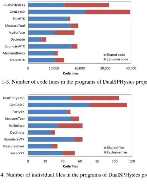
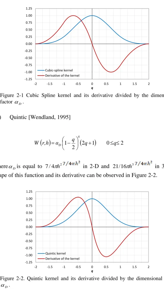
Figure 1-1. Floating-Point Operations per Second for the CPU and GPU (source: CUDA Programming Guide v6.5). ... 6 Figure 1-2. DualSPHysics website. ... 9 Figure 1-3. Number of code lines in the programs of DualSPHysics project. ... 10 Figure 1-4. Number of individual files in the programs of DualSPHysics project. ... 10 Figure 2-1 Cubic Spline kernel and its derivative divided by the dimensional factor D. ... 15 Figure 2-2. Quintic kernel and its derivative divided by the dimensional factor
D
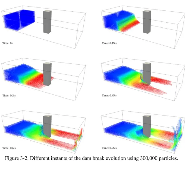
. ... 15 Figure 3-1. Conceptual diagram summarising the implementation of a SPH code. ... 27 Figure 3-2. Different instants of the dam break evolution using 300,000 particles. ... 29 Figure 3-3. Sketch of the Cell-linked list (CLL). ... 32 Figure 3-4. Sketch of the Verlet list (VL). ... 34 Figure 3-5. Computational runtime of different approaches for neighbour list. .. 35 Figure 3-6. Memory requirements of different approaches for neighbour list. .... 35 Figure 3-7. Improvement in time using VLC and VLX compared to CLL. All cases
were calculated with N=31,239. ... 36 Figure 3-8. Allocated memory in CLL, VLX and VLC. All cases were calculated
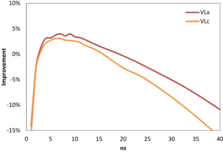
with N=31,239. ... 36 Figure 3-9. Improvement comparison between VLX and VLC referred to CLL. ... 37
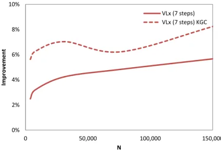
Figure 3-10. Comparison between VLX with and without kernel gradient correction (KGC). The improvement is referred to CLL. ... 38
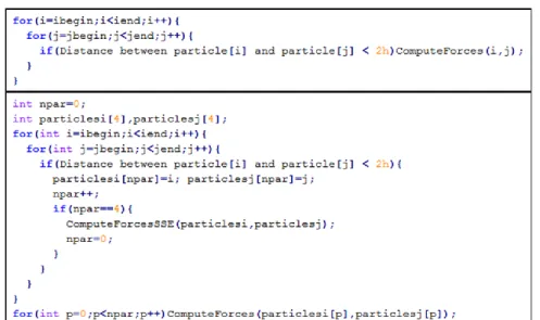
Figure 4-1. Interaction cells in 3D without (left) and with (right) symmetry in particle interactions. Each cell interacts with 14 cells (right) instead of 27 (left). ... 42 Figure 4-2. Sketch of 3D interaction with close cells using symmetry. The volume searched using cells of side 2h (left panels) is bigger than using cells of side h (right panels). ... 43 Figure 4-3. Sketch Pseudocode in C++ showing the force computation between the particles of two cells without vectorial instructions (up) and grouping in blocks of 4 pair-wise of interaction using SSE instructions (down). ... 44 Figure 4-4. Example of dynamic distribution of cells (in blocks of 4) among 3 execution threads according to the execution time of each cell. ... 45 Figure 4-5. Speedup achieved on CPU for different number of particles (N) when applying symmetry, the use of SSE instructions. Two different cell sizes (2h and
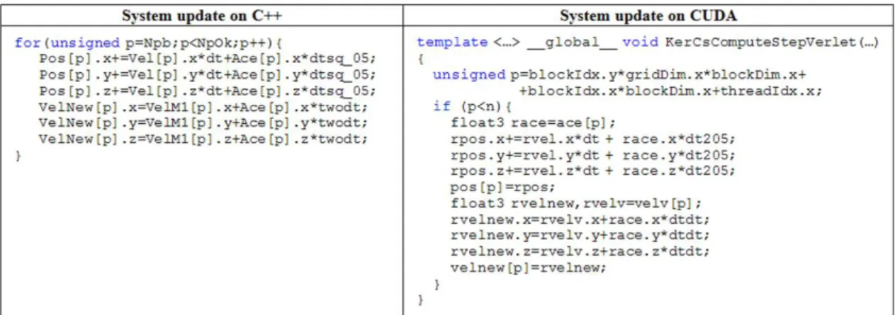
2h/2) were considered. ... 47 Figure 4-6. Speedup achieved on CPU for different number of particles (N) with different OpenMP implementations (using 8 logical threads) in comparison with the most efficient single-core version that includes all the previous optimizations. ... 48 Figure 5-1. Grid of thread blocks in CUDA (source: CUDA Programming Guide v6.5) ... 50 Figure 5-2. Memory hierarchy (source: CUDA Programming Guide v6.5) ... 51 Figure 5-3. Conceptual diagram of the partial (left) and full (right) GPU implementation of the SPH code. ... 52 Figure 5-4. Example of the Neighbour list procedure. ... 54 Figure 5-5. Pseudocode of the System update procedure implemented on CPU and GPU. ... 55 Figure 5-6. Pseudocode of the Particle interaction procedure implemented on CPU and GPU. ... 56 Figure 5-7. Occupancy of the GPU for different number of registers with a variable and a fixed block size of 256 threads. ... 58 Figure 5-8. Interaction cells in 3D without symmetry but using 9 ranges of three consecutive cells (right) instead of 27 cells (left). ... 60 Figure 5-9. Computational runtimes (in seconds) using GTX 480 for different GPU implementations (partial, full and optimized) when simulating 500,000 particles. ... 63 Figure 5-10. Memory usage for different GPU versions implemented in DualSPHysics. ... 65 Figure 5-11. Runtimes for different CPU and GPU implementations. ... 65
Figure 5-12. Runtime for CPU and different GPU cards. ... 66 Figure 5-13. Speedups of GPU against CPU simulating 1 million particles. ... 67 Figure 5-14. Computational runtime distribution on CPU and GPU simulating 1 million particles. Neighbour List corresponds to blue bars, Particle Interaction to red bars and System Update to the green bars. ... 67 Figure 5-15. Maximum number of particles simulated with different GPU cards using DualSPHysics code. ... 68 Figure 6-1. Scheme of technologies and its scope of application. ... 70 Figure 6-2. Domain subdivision in four processes. ... 73 Figure 6-3. Example of subdivision of a domain (halos and edges). ... 74 Figure 6-4. Scheme of the communications among 3 MPI processes. ... 76 Figure 6-5. Example of the dynamic balancing scheme between 2 GPUs. ... 78 Figure 6-6. Testcase1: Dam break flow impacting on a structure... 79 Figure 6-7. Testcase2: Dam break flow. ... 80 Figure 6-8. Different instants of the simulation of testcase1 when using the dynamic load balancing according to the number of particles. ... 81 Figure 6-9. Distribution of the fluid particles and execution times of force computation among the 3 GPUs of system #1a using load balancing according to the number of particles. ... 82 Figure 6-10. Distribution of the fluid particles and execution times of force computation among the 3 different GPUs of system #1b using load balancing according to the number of particles. ... 82 Figure 6-11. Distribution of the fluid particles and execution times of force computation among the 3 different GPUs of system #1b using load balancing according to the computation time. ... 83 Figure 6-12. Execution times of the 3 GPUs of the system #1b used individually and together applying dynamic load balancing. ... 83 Figure 6-13. Speedup for different number of GPUs using strong and weak scaling with the hardware systems #1, #2 and #3. ... 85 Figure 6-14. Percentage of time dedicated to tasks exclusive of the multi-GPU executions using the system #3. ... 86 Figure 6-15. Percentage of the computational time dedicated to specific MPI tasks simulating 16M particles using different number of Tesla M2050 GPUs (left) and simulating different number of particles with 16 Tesla M2050 (right). ... 87
Figure 6-16. Percentage of time dedicated to tasks exclusive of the multi-GPU executions including the latest improvements (using the system #2). ... 88 Figure 6-17. Maximum number of particles that can be simulated for the testcase2 with the system s #1, #2 and #3. ... 89 Figure 6-18. Realistic dimensions of the oil rig simulated in the application. ... 90 Figure 6-19. Different instants (2.2s, 3.2s and 10s) of the simulation of a large wave interacting with an oil rig using more than 109 particles... 90 Figure 7-1. Testbed to study problems of precision. ... 93 Figure 7-2. Different instants of the simulation of the testbed. ... 95 Figure 7-3. Relative error in the distance between two particles interacting using double and single precision for different particle positions. ... 95 Figure 7-4. Different instants of the previous simulation improving precision in the position of the particles. ... 97 Figure 7-5. Relative error in the position of the particles for different distances to zero and using different approaches. ... 98 Figure 7-6. Loss of efficiency compared with simple precision simulations using a 3D dam-break with 4M particles. ... 99 Figure 7-7. Percentage of occupancy according to the number of registers and compute capability of GPU. ... 100
Figure B-1. Generation of a 2D triangle. ... 117 Figure B-2. Discretization accuracy for different number of particles.The absolute measures of the object are 0.39 x 0.46 x 0.42. ... 117 Figure B-3. Some predefined objects: box, sphere, cylinder, prism,… ... 118 Figure B-4. Basic shapes “solid” and “face”. ... 118 Figure B-5. Mixer: 3D model (left) and point distribution (right). ... 119 Figure B-6. Filling an irregular beach with fluid. ... 120 Figure B-7. Example of rotation and scaling of a 3D model. ... 121 Figure B-8. Creating a balustrade starting from a primitive element. ... 121 Figure B-9. Merging objects with different label. ... 121 Figure B-10. Gravity center and inertia (lower pannel) computed starting from different particle distributions (upper pannel). ... 122 Figure B-11. Different initial configurations depending on the value of lattice for fluid (blue points) and boundary (black points) particles. ... 123
Figure B-12. Initial density distribution. ... 124 Figure B-13. Mixing of two fluids. ... 124 Figure B-14. Different instants of a pendulum movement (rotational, circular and rectilinear sinusoidal). ... 125 Figure B-15. Mixer as an example of hierarchy of movements. ... 126 Figure B-16. Normal vector (n) computation for a triangle. ... 126 Figure B-17. Normal vector computation for a 3D object. ... 127 Figure B-18. Sink with floating object (polygons and particles). ... 128 Figure B-19. Execution runtimes for the Sink. ... 129 Figure B-20. Mixer (polygons and particles). ... 129 Figure B-21. Execution runtimes for the Mixer. ... 129 Figure B-22. Pump (polygons and particles). ... 130 Figure B-23. Execution runtimes for the Pump. ... 130 Figure B-24. Mini Cooper (polygons and wire). ... 131 Figure B-25. Execution runtimes for the Mini Cooper. ... 131
Figure C-1. Visualization of density from a fluid block of particles. ... 133 Figure C-2. Example of graph with wave elevation at a specific position. ... 134 Figure C-3. Visualizes the wave elevation for a slice of fluid. ... 134 Figure C-4. Conversion of points to surfaces, from particles to isosurface. ... 135 Figure C-5. Original isosurface of fluid (left) and simplified isosurface by Decimate program with a reduction to 10%. ... 136 Figure C-6. Floating body movement represented using a box. ... 137 Figure C-7. Appliaction of MeasureBoxes to measure a flow at complex terrain. ... 138 Figure C-8. Waves interaction with a coastal structure consisting of antifers and trajectories of fluid particles between antifers. ... 139
LIST OF TABLES
Table 3-1. Generic modules of a SPH code using cell-linked lists (CLL) and Verlet lists (VL). ... 31 Table 4-1. Speedup achieved on CPU simulating 300,000 particles when using 4 and 8 threads compared to the single CPU version. ... 48 Table 5-1. Technical specifications of GPUs according to the compute capability. ... 58 Table 5-2. List of variables needed to calculate forces. ... 59 Table 5-3. Improvement achieved on GPU simulating 1 million particles when applying the different GPU optimizations using GTX 480 and Tesla 1060. ... 62 Table 5-4. Results of the CPU and GPU simulations. ... 64 Table 5-5. Specifications of different execution devices. ... 66 Table 6-1. Features of the different systems used. ... 80 Table 6-2. Formulae to measure efficiency and scalability... 84 Table 7-1. Double precision implementations ... 98
Table A-1. List of source files of DualSPHysics code. ... 107 Table A-2. List of source files of DualSPHysics code not related to the SPH solver. ... 108 Table A-3. List of source files of DualSPHysics code for the SPH execution. . 108 Table A-4. List of source files of DualSPHysics code for the SPH execution on CPU. ... 109 Table A-5. List of source files of DualSPHysics code for the SPH execution on GPU. ... 109 Table A-6. List of execution parameters of DualSPHysics... 113
LIST OF ACRONYMS
API: Application Program Interface.
ASCII: American Standard Code for Information Interchange.
BSC-CNS: Barcelona Supercomputing Center - Centro Nacional de Supercomputación
CAD: Computer-aided design.
CFD: Computational Fluid Dynamics.
CFL: Courant-Friedrich-Levy condition.
CLL: Cell-linked List
CPU: Central Processing Unit.
CSV: Comma-separated Values.
CUDA: Compute Unified Device Architecture.
DEM: Discrete Element Method.
DSP: Digital Signal Processors.
ECC: Error-correcting code memory.
FLOP: Floating-point Operations Per Second.
FPGA: Field Programmable Gate Array.
GC: Centre of gravity.
GPGPU: General-Purpose Computing on Graphics Processing Units.
GPU: Processing Graphics Units.
HPC: High Performance Computing.
KGC: Kernel Gradient Correction.
MD: Molecular Dynamics.
MPI: Message Passing Interface.
NL: Neighbour List step.
OpenMP: Open Multi-Processing.
PI: Particle Interaction step.
SIMD: Single Instruction, Multiple Data.
SM: Streaming Multiprocessor.
SPH: Smoothed Particle Hydrodynamics.
SPS: Turbulence: Sub-Particle Scale Turbulence.
SU: System Update step.
VL: Verlet list.
VTK: Visualization ToolKit.
WCSPH: weakly-compressible SPH.
1.
INTRODUCTION
In this first chapter, a general overview of the numerical methods and, more specifically, of the Smoothed Particle Hydrodynamics (SPH) method is provided. The advantages and disadvantages of the SPH methods when compared with other methods are also described. Furthermore, different High Performance Computing techniques are presented to accelerate the SPH method. Finally, the DualSPHysics code is presented.
1.1
N
UMERICAL MODELINGNature can be modelled looking for analytical solutions of the equations that define a system (or mathematical model). Once the equations are validated, the behaviour of the system can be predicted tuning some parameters and imposing a set of initial conditions. The numerical modelling looks for solving these equations in a numerical way instead of analytically. So that, designing algorithms that use numbers and simple mathematical rules that can simulate complex processes of the real world. The numerical simulation is a powerful tool that allows for understanding the behaviour of complex systems and even for predicting their evolution starting from initial conditions. Numerical modelling becomes more important with the arrival of the computers since these machines can perform thousands of million mathematical operations per second. This allows for the simulation of very complex systems in few time using simple mathematical operations.
Computational Fluid Dynamics (CFD) is a branch of fluid mechanics that studies the behaviour of the fluids using numerical modelling. The main advantage of this technique is the capability to simulate complex scenarios and provide physical data that can be difficult, or even impossible, to measure in a real model. Despite of the accuracy of the numerical models, these cannot replace the
construction of scale models, but they can reduce significantly the number of physical tests. This leads to an important saving since the construction of physical models is very expensive and slow.
There are two numerical approaches to describe the fluid motion; Eulerian and Lagrangian. The Eulerian approach solves the equations at the fixed nodes of a mesh. In the Lagrangian description, the positions where equations are solved move with the fluid and a fixed mesh is not used. The meshbased methods (finite elements, finite differences and finite volumes) are currently very robust, well developed and have been applied to a wide range of applications providing highly accurate results. These meshbased methods are ideal for systems where the domain is perfectly defined and for simulations where the boundaries remain fixed. However the creation of the mesh can be very inefficient if the system is complex. In recent years, numerous meshless methods have appeared and grown in popularity as they can be applied to problems that are highly nonlinear in arbitrarily complex geometries and are difficult for mesh-based methods. Within the meshless methods now available, Smoothed Particle Hydrodynamics (SPH) is, possibly, the most popular and has attained the required level of maturity to be used for engineering purposes.
1.2
S
MOOTHEDP
ARTICLEH
YDRODYNAMICSSmoothed Particle Hydrodynamics (SPH) is a Lagrangian meshless method that is increasingly used for an extensive range of applications within the field of Computational Fluid Dynamics (CFD). Originally invented for astrophysics during the seventies [Lucy, 1977; Gingold and Monaghan, 1977], it has been applied in many different fields including fluid dynamics and solid mechanics. The method uses particles to represent a fluid and these particles move according to the governing dynamics. More complete description of the SPH formulation is found in Chapter 2. When simulating free-surface flows, the Lagrangian nature of SPH allows the domain to be multiply-connected, with no need of a special treatment of the surface, making the technique ideal for studying violent free-surface motion.
SPH has been used to describe a variety of free-surface flows (wave propagation over a beach, plunging breakers, impact on structures and dam breaks). [Monaghan, 1994] presented the first attempt to study free-surface flows. Monaghan also studied the behaviour of gravity currents ([Monaghan, 1996]),
solitary waves ([Monaghan et al., 1999]) and wave arrival at a beach ([Monaghan and Kos, 1999]). Later on, the model was applied to the study of the wave-structure interaction such as in [Colagrossi and Landrini, 2003] that considered the study of interfacial flows. The classical dam-break problem was also studied in 3D by [Gómez-Gesteira and Dalrymple, 2004]. Within the area of coastal engineering, SPH was firstly employed to study wave-breakwater interaction in [Gotoh et al., 2004] and [Shao, 2005], and to predict wave impact pressure due to sloshing waves in [Khayyer and Gotoh, 2009].
However, the high computational cost is the most important drawback of this technique. Thus, a short period of physical time applications requires a large execution time when running on a single Central Processing Unit (CPU) due to the large number of interactions for each particle at each timestep. This has hindered the development of SPH and its industrial use to solve real problems. Hence, the ability to perform computations involving millions of particles in a reasonable time is essential to perform simulations that are industrially relevant. However, this is only possible if some hardware acceleration techniques are employed.
1.3
H
IGHP
ERFORMANCEC
OMPUTINGHigh Performance Computing (HPC) is a very dynamic field that deals with the study and usage of new computational resources and technologies. Its aim is to solve very complex problems that require high computational capacity so that cannot be solved with conventional computer systems, making necessary the use of clusters or supercomputers. A supercomputer is a computer with a very high computational speed dedicated on the execution of parallel operations and designed for intensive computation. These are extremely expensive machines. On the other hand, a cluster is a collection of computers connected through a high speed network and considered as a single machine. This is a cheaper option as it can be integrated by more conventional machines, which currently have high performance at very low prices. They also offer the possibility to extend their computing capacity, theoretically unlimited, by simply adding more computers. HPC includes multiple techniques of parallel computing and distributed computing. In the main, parallel computing consists of executing several operations simultaneously.
This parallelism can be applied at instruction-level, since current processors divide the execution of an instruction in several stages, so they can keep running several instructions at different stages (instruction pipelines). In addition, the superscalar microprocessors can execute multiple instructions simultaneously when there is no data dependency among them. The task-level parallelism consists of dividing a volume of data into different computing nodes to perform the same set of operations. Finally, the task-level parallelism distributes the execution of different computations, on the same or different data, among multiple processing units.
Parallel computing can be applied with hardware of shared memory in which a machine has one or more processors that use the same memory space. In this case the more extended tools of programming are pthreads [Buttlar et al., 1996] and OpenMP [Chandra et al., 1996; Chandra et al., 2002] that can be considered as the standard for this kind of systems with shared memory, due to the advantages over other standard parallel-programming models [Dagum and Menon, 1998]. Parallel computing can be also applied with systems of distributed memory in which each processor is associated with a memory space and cannot directly access to the memory associated with other processors. In these systems, the data exchange between processors must be carried out explicitly using a message passing model. The most common options for this kind of programming are PVM [Geist et al., 1994], BSP [Bisseling, 2004] and MPI [Pacheco, 1996; Snir et al., 1998; Gropp et al., 1999] that is the standard one.
It is also important to note that in recent years, the use of special-purpose processors as general purpose parallel systems are becoming increasingly important in HPC. Hence, Processing Graphics Units (GPU), Digital Signal Processors (DSP), Field Programmable Gate Array (FPGA) and other systems are used as scientific computer systems rather than for its original purpose.
The following explains in more detail the main HPC techniques used to accelerate SPH.
1.3.1
OpenMP (Open Multi-Processing)
OpenMP [http://www.openmp.org] is a model of parallel programming for systems of shared memory. It provides an Application Program Interface (API) in C, C++ and Fortran applications. OpenMP is a portable and flexible programming interface where multiple threads of execution perform tasks
defined by OpenMP directives. Its implementation does not involve major changes in the code. Using OpenMP, multiple threads for a process can be easily created. These threads are distributed among all the cores of the CPU sharing the memory. Thus, there is no need to duplicate data or to transfer information among threads. For these reasons OpenMP is the best option to optimize the performance of the multiple cores of the current CPUs [Clark, 1998].
1.3.2
MPI (Message Passing Interface)
MPI is a message-passing library specification for parallel computers and clusters where a distributed memory system is used. MPI is not a language or a compiler or a specific implementation, it simply defines a library of functions that can be called from C, C++, and Fortran programs. In this parallel programming model, an execution consists of one or more processes that communicate by calling routines of a library to send and receive messages among processes. Although designed for distributed memory systems, its use with shared memory systems can lead to an improvement since MPI encourages memory locality. The use of MPI is typically combined with OpenMP in clusters by using a hybrid communication model. In this way, within each machine, the processors directly access the shared memory and the message exchange with MPI is used to share information among processes of different machines.
The first implementation of MPI standard was MPICH [http://www-unix.mcs.anl.gov/mpi/mpich1]. Other implementations are LAM-MPI [http://www.lam-mpi.org/] and more recently, OpenMPI [http://www.open-mpi.org] that is an open-source distribution of the MPI2 specification.
1.3.3
GPGPU (General-Purpose Computing on Graphics
Processing Units)
GPGPU involves the study and use of parallel computing ability of a GPU to perform general purpose programs. Graphics Processing Units are powerful parallel processors originally designed for graphics rendering. Due to the development of the video games market and multimedia, their computing power has increased much faster than CPUs (see Figure 1-1). Therefore GPUs can be used for scientific applications achieving speedups of 100x or more. This joined to their very low cost and that GPUs can be used on a personal computer made GPGPU very popular in recent years [Owens et al., 2007; Nickolls and Dally, 2010]. In fact, new computation centres based on GPUs are emerging driven by
their computing power and comparatively low energy costs per FLOP (Floating-point Operations Per Second) [McInstosh-Smith et al., 2012]. Indeed, the current number two of the TOP500 List of the world’s top supercomputers released in June 2014 [http://www.top500.org/lists/2014/06] is Titan, a Cray XK7 system that has 560,640 processors, including 18,688 Nvidia K20x accelerator GPU cards.
Figure 1-1. Floating-Point Operations per Second for the CPU and GPU (source: CUDA Programming Guide v6.5).
GPUs are optimized for floating-point parallel operations, it is important to note that not all applications are suitable for GPU, only those that exhibit a high degree of parallelism. In addition, the features of the GPU architecture need to be taken into account to obtain the maximum performance. While CPUs are designed for an efficient random memory access, GPUs provide a more restrictive memory access and a careful usage of the memory hierarchy is fundamental. This requires a new implementation of the algorithms used in CPU for an efficient use in GPUs.
Much of the success of GPGPU is the appearance of general purpose programming languages and APIs such as Brook and CUDA since they provided an easier access to the computing power of these devices. Brook was a compiler and runtime implementation of a stream programming language for modern graphics hardware of ATI Technologies. CUDA (Compute Unified Device
Architecture) is both a programming environment and language for parallel computing specifically for Nvidia GPUs [Nickolls et al., 2008; CUDA Programing Guide]. Currently CUDA is the most popular programming graphics model due to the large amount of documentation and utilities that can be found in the CUDA web (https://developer.nvidia.com/cuda-zone).
The framework called OpenCL (Open Computing Language) [Khronos, 2009] is becoming increasingly important in GPGPU. OpenCL is a framework to code programs that are executed across heterogeneous platforms including GPUs, CPUs, DSPs, FPGAs and other processors. It is an open standard maintained by Khronos Group and adopted by the most important technology companies such as Intel, AMD and Nvidia.
1.4
D
UALSPH
YSICS PROJECTSPHysics was an open-source SPH model developed by researchers at the Johns Hopkins University (US), the University of Vigo (Spain), the University of Manchester (UK) and the University of Rome, La Sapienza. The software is available to download from www.sphysics.org, a complete guide of the FORTRAN code is found in [Gómez-Gesteira et al., 2012a; Gómez-Gesteira et al., 2012b]. The SPHysics code was validated for different problems of wave breaking [Dalrymple and Rogers, 2006], dam-break behaviour [Crespo et al., 2008], interaction with coastal structures [Gómez-Gesteira and Dalrymple, 2004] or with a moving breakwater [Rogers et al., 2010]. A shallow water version was also developed [Vacondio et al., 2012; Vacondio et al., 2013a]. Although SPHysics allows modelling problems with high resolution, the main problem for the application to real engineering problems is its high computational cost, therefore SPHysics is rarely applied to large domains. Hardware acceleration and parallel computing are required to make codes such as SPHysics more useful and versatile.
The code DualSPHysics has been developed by starting from the FORTRAN SPH formulation implemented in SPHysics, this code was considered robust and reliable but not optimised for large simulations. DualSPHysics is implemented in C++ and CUDA and is designed to launch simulations either on multiple CPUs using OpenMP or on a GPU. The GPU portion of DualSPHysics implements the most appropriate parallelisation to maximise speedup during particle interaction computation.
The code can be executed either on the CPU or on the GPU since all computations have been implemented both in C++ for CPU simulations and in CUDA for the GPU simulations. The philosophy underlying the development of DualSPHysics is that most of the source code is common to CPU and GPU which makes debugging straightforward as well as the code maintenance and new extensions. This allows the code to be run on workstations without a CUDA-enabled GPU, using only the CPU implementation. On the other hand, the resulting codes should be necessarily different since code developers have considered efficient approaches for every processing unit. As explained below, the same programming strategy can be efficient on a CPU but inefficient on a GPU (or vice versa). Thus, comparisons between the performances of both approaches are more reliable since appropriate optimisations have been considered for every case.
The first rigorous validation of the GPU implementation of DualSPHysics code was presented in [Crespo et al., 2011]. The code has been developed to simulate real-life engineering problems using SPH models such as the computation of forces exerted by large waves on the urban furniture of a realistic promenade ([Barreiro et al., 2013]) or the study of the run-up in an existing armour block sea breakwater ([Altomare et al., 2014a]). Other recent examples of the study of wave-structure interaction, by means of the DualSPHysics model, are the works of [Ren et al., 2014], where the SPH model is validated against other available numerical results and against experimental data for wave damping over porous seabed with different levels of permeability. Other recent example is the work of [St-Germain et al., 2014] to investigate the hydrodynamic forces induced by the impact of rapidly advancing tsunami like hydraulic bores.
DualSPHysics is an open-source code developed and redistributed under the terms of the GNU General Public License as published by the Free Software Foundation (www.gnu.org/licenses/). The software is availab