Bayesian Parameter Estimation
and Variable Selection
for Quantile Regression
A thesis submitted for the degree of
Doctor of Philosophy
by
Craig Reed
Department of Mathematics
School of Information Systems,
Computing and Mathematics
Abstract
The principal goal of this work is to provide efficient algorithms for implementing the Bayesian approach to quantile regression. There are two major obstacles to overcome in order to achieve this. Firstly, it is necessary to specify a suitable likelihood given that the frequentist approach generally avoids such specifications. Secondly, sampling methods are usually required as analytical expressions for posterior summaries are generally unavailable in closed form regardless of the prior used.
The asymmetric Laplace (AL) likelihood is a popular choice and has a direct link to the frequentist procedure of minimising a weighted absolute value loss function that is known to yield the conditional quantile estimates. For any given prior, the Metropolis Hastings algorithm is always available to sample the pos-terior distribution. However, it requires the specification of a suitable proposal density, limiting it’s potential to be used more widely in applications.
It is shown that the Bayesian quantile regression model with the AL likelihood can be converted into a normal regression model conditional on latent parameters. This makes it possible to use a Gibbs sampler on the augmented parameter space and thus avoids the need to choose proposal densities. Using this approach of introducing latent variables allows more complex Bayesian quantile regression models to be treated in much the same way. This is illustrated with examples varying from using robust priors and non parametric regression using splines to allowing model uncertainty in parameter estimation. This work is applied to comparing various measures of smoking and which measure is most suited to predicting low birthweight infants. This thesis also offers a short tutorial on the R functions that are used to produce the analysis.
Declaration
I declare that this thesis was composed by myself and that the work contained therein is my own, except where explicitly stated otherwise in the text.
Acknowledgements
I would like to thank Professor David B. Dunson for his suggestions regarding Bayesian variable selection for quantile regression, Dr Paul Thompson for giving me the R code to implement the Metropolis Hastings algorithm for the splines example, Professor Janet Peacock for providing the birthweight data and my supervisors Dr Keming Yu and Dr Veronica Vinciotti for their supervision of this work. My thanks also go to all fellow students and staff who made my time at Brunel a thoroughly enjoyable experience. Finally, my thanks go to my parents and friends who provided unwavering support throughout my studies.
Table of Contents
List of Tables 3
List of Figures 5
List of Algorithms 6
Chapter 1 Introduction 7
1.1 Why use quantile regression? . . . 7
1.2 Examples of Cases where Quantile Regression is Useful . . . 8
1.3 The Frequentist Approach . . . 9
1.4 The Bayesian Approach . . . 12
1.5 Thesis Outline . . . 15
Chapter 2 Bayesian Quantile Regression using Data Augmentation 17 2.1 Introducing the Latent Variables . . . 17
2.2 Engel data: Comparing Augmented Posterior Summaries with Fre-quentist Estimate/ Marginal Posterior Mode . . . 21
2.3 Stackloss data: Comparison of Gibbs sampler and Metropolis-Hastings algorithm . . . 23
2.4 Bayesian Quantile Regression with Natural Cubic Splines . . . 24
2.5 Summary . . . 33
Chapter 3 An Application in Epidemiology:
In-fants than the Reported Number of Cigarettes? 35
3.1 Introduction and Method . . . 35
3.2 Results . . . 38
3.3 Conclusion of Study . . . 46
Chapter 4 Bayesian Variable Selection for Quantile Regression 47 4.1 Introduction and Method . . . 47
4.1.1 QR-SSVS algorithm . . . 50
4.2 Revisiting the Stack Loss Data . . . 51
4.3 Application to Boston Housing data . . . 55
4.4 Summary . . . 58
Chapter 5 Conclusions and Future Research 59 5.1 A Summary of this Thesis . . . 59
5.2 Extensions . . . 61
5.2.1 Shape parameter σ . . . 61
5.2.2 Multiple values of τ . . . 62
5.2.3 Prediction . . . 64
5.2.4 Posterior mode using the EM algorithm . . . 65
5.3 Recommendations . . . 67
Appendix A Practical Implementation in R 75 A.1 Introduction . . . 75
A.2 Using Gibbs Sampling for Bayesian Quantile Regression in R . . . 76
A.2.1 MCMCquantreg . . . 76
A.2.2 SSVSquantreg . . . 79
List of Tables
2.1 Comparison of frequentist estimate (also marginal posterior mode) and posterior mean and median, estimated from the Gibbs sample by retaining only the β values. The summary statistics are calcu-lated from 11,000 iterations with the first 1,000 discarded. . . 22 2.2 Comparison of Gibbs sampler and Metropolis-Hastings(MH). The
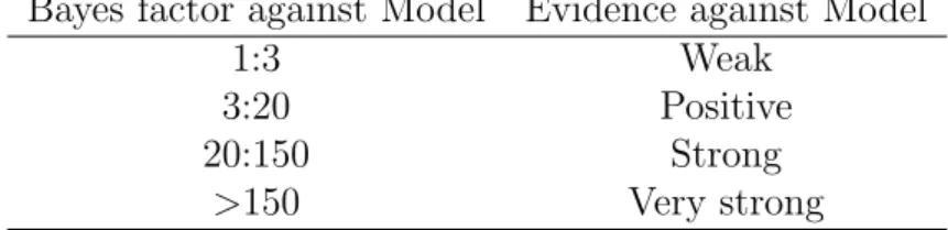
posterior means were recorded together with the 95% highest pos-terior density (HPD) intervals (in parentheses). . . 25 3.1 Bayes factors against Model 1: Model 1 number of cigarettes vs.
Model 2 cotinine. . . 42 3.2 Interpretation of Bayes factors from Kass and Raftery (1995). . . 42 3.3 Bayes factors against Model 1: Model 1 null model vs. Model 2
cotinine difference. . . 44 3.4 Bayes factors against Model 1 for passive smokers: Model 1 null
model vs. Model 2 cotinine. . . 44 4.1 Models visited by QR-SSVS with their estimated posterior
proba-bility. The top 3 models are displayed forτ ∈ {0.05,0.25,0.5,0.75,0.95}. 53 4.2 Models visited by QR-SSVS atτ = 0.5 with their estimated
poste-rior probability. The top 3 models are displayed for the hyperpposte-riors
4.3 Marginal inclusion probabilities (MIPs), posterior summaries and corresponding frequentist estimates (based on the full model) of the Boston Housing data, presented forτ = 0.5. . . 56 4.4 The 5 models with the highest estimated posterior probability. The
List of Figures
2.1 Stackloss data: Comparing autocorrelation of Gibbs and MH at
τ = 0.5. The top row corresponds to the Gibbs sampler, the bottom row to MH with optimal settings. . . 26 2.2 Bayesian nonparametric regression using NCS for τ = 0.95. The
blue curve is obtained from our Gibbs sampler, the red curve is obtained from MH. The dashed black curve is the true underlying curve. . . 30 2.3 Plot of the first 10,000 iterations of the Metropolis Hastings chains,
plotted for g1. . . 31
2.4 Plot of the first 100 iterations of the Gibbs chains, plotted for g1. 32
3.1 Scatterplot of cotinine level at booking against adjusted birth-weight. The points include all those classed as smokers with a cotinine level above 15ng/ml. . . 40 3.2 Plot of posterior mean cotinine against quantile. The shaded area
is the 95% HPD interval. . . 41 3.3 Plot of posterior mean difference in cotinine against quantiles.
Shaded region is 95% HPD interval. . . 43 3.4 Posterior mean of cotinine for passive smokers against quantile.
Shaded region is 95% HPD interval. . . 45 A.1 R plot obtained by the plotfunction on an object of class qrssvs. 82
List of Algorithms
2.1 Gibbs sampler for augmented quantile regression model with initial values for β. Draws M burn in samples followed by an additional N samples for inference. . . 20 2.2 Gibbs sampler for augmented quantile regression model with initial
values for w. Draws M burn in samples followed by an additional N samples for inference. . . 21 2.3 Gibbs sampler for quantile regression with natural cubic splines.
Draws M burn in samples and N samples for inference. . . 29 3.1 Gibbs sampler for augmented quantile regression model under
in-dependent Cauchy priors onβ. Draws M burn in samples followed by an additional N samples for inference. . . 37 3.2 Chib’s method for calculating approximate marginal likelihood l(y). 38 4.1 Component of QR-SSVS algorithm that updates the vectorγ. . . 51 4.2 Stochastic search variable selection for quantile regression model.
Draws M burn in samples followed by an additional N samples for inference. . . 52 5.1 Gibbs sampler for augmented quantile regression model with shape
parameter σ. Draws M burn in samples followed by an additional N samples for inference. . . 63 5.2 The EM algorithm for finding the posterior mode under a N(b0,B0−1)
prior where each yi has an AL distribution with skewness τ and
Chapter 1
Introduction
1.1
Why use quantile regression?
Since the introduction of quantile regression in a paper by Koenker and Bassett (1978), there has been much interest in the field. Quantile regression is used when an estimate of the various quantiles (such as the median) of a conditional distribution is desired. It can be seen as a natural analogue in regression analysis to the practice of using different measures of central tendency and statistical dispersion to obtain a more comprehensive and robust analysis (Koenker, 2005). To get an idea of the usefulness of quantile regression, note the identity linking the conditional quantiles to the conditional mean:
E(y|x) =
Z 1
0
Qτ(y|x)dτ, (1.1)
where E(y|x) denotes the conditional expectation of y given x and Qτ(y|x)
de-notes the conditional τth quantile of y given x. In essence, this result implies that traditional mean regression is a summary of all possible quantile regressions. Hence, a simple mean regression analysis can be insufficient to describe the com-plete relationship between yand x. This is demonstrated empirically by Min and Kim (2004), who simulate data based on a wide-class of non Gaussian error distri-butions. They conclude that simple mean regression cannot satisfactorily capture the key properties of the data and that even the conditional mean estimate can be misleading.
known that the mean is not a robust estimate when the underlying distribution is asymmetric or has non-negligible probabilities of extreme outcomes (the distri-bution has long tails). In such cases, the median (central quantile) offers a more robust estimate of the centre of the distribution. Situations like these are com-monly encountered in real datasets from a number of disciplines such as social sciences, economics, medicine, public health, financial return, environment and engineering. Examples are presented in the next section.
This thesis focuses solely on the problem of parameter estimation in Bayesian quantile regression models, firstly assuming the regression model is fixed and then later relaxing this assumption. In addition, this thesis focuses on quantile regres-sion models specified linearly in terms of the regresregres-sion parameters. However, the ideas presented in the next chapter can be extended to handle nonlinear quantile regression under a Bayesian framework. For a discussion about using these models for prediction and other extensions, see Chapter 5.
1.2
Examples of Cases where Quantile
Regres-sion is Useful
Quantile regression enjoys some wide ranging applications. Here are some of them.
• Many asymmetric and long-tailed distributions have been used to model the innovation in autoregressive conditional heteroscedasticity (ARCH) models in finance. Specifically, the conditional autoregressive value at risk (CAViaR) model introduced by Engel and Manganelli (2004) is a very popular time series model for estimating the value at risk in finance.
• In ecology, there exist complex interactions between different factors affect-ing organisms that cannot all be measured and accounted for in statistical models. This leads to data which often exhibit heteroscedasticity and as such, quantile regression can give a more complete picture about the under-lying data generating mechanism (Cade and Noon, 2003).
• In the study of maternal and child health and occupational and environ-mental risk factors, Abrevaya (2001) investigates the impact of various de-mographic characteristics and maternal behaviour on the birthweight of infants born in the U.S. Low birthweight is known to be associated with a wide range of subsequent health problems and developmental markers.
• Based on a panel survey of the performance of Dutch school children, Levin (2001) found some evidence that for those individuals within the lower por-tion of the achievement distribupor-tion, there is a larger benefit of being placed in classes with individuals of similar ability. This benefit decreases mono-tonically as the quantile of interest is increased.
• Chamberlain (1994) infers that for manufacturing workers, the union wage premium, which is at 28 percent at the first decile, declines continuously to 0.3 percent at the upper decile. The author suggests that the location shift model estimate (least squares estimate) which is 15.8 percent, gives a misleading impression of the union effect. In fact, this mean union premium of 15.8 percent is captured primarily by the lower tail of the conditional distribution.
These examples demonstrate the fact that quantile regression can be an im-portant part of any statistician’s toolbox. For more details and examples, see Yu et al. (2003).
1.3
The Frequentist Approach
The linear parametric model specifies the conditional quantiles as
Qτ(yi|xi) = xiTβ(τ), i= 1, . . . , n, (1.2)
wherexi denotes the ith column of then×(p+ 1) design matrix Xmade up of p predictors and the intercept andβ(τ) denotes the (p+ 1)×1 vector of associated regression parameters for a fixed value of τ.
In classical (frequentist) quantile regression estimation, the aim is to find an estimator βˆ(τ) of β(τ). This is often done without relying on a specification of the form of the residual distribution such as the assumption that the residuals are normally distributed with mean 0 and varianceσ2. Analysis may focus on one
value of τ, sayτ = 0.5 for the conditional median, or a set of values for τ. If just one value of τ is of interest, Koenker and Bassett (1978) show that minimising the loss function given by
n X i=1 ρτ(yi−xiTβ), (1.3) where ρτ(u) := τ u if u≥0, (1−τ)|u| if u <0. (1.4)
leads to the τth regression quantile. In the case of multiple quantile regressions, the procedure of minimising (1.3) could be repeated with different values of τ. More generally, the entire path of β(τ) could be modelled through the quantile regression process in which τ becomes a continuous variable in (0,1). Koenker and Bassett (1978) show that the problem of minimising (1.3) can be converted into a linear program and give details on how to solve it efficiently for any or all τ ∈ (0,1). This procedure now comes as standard in the quantreg package (Koenker, 2009) for R (R Development Core Team, 2010).
Without specifying the form of the residual distribution, frequentist inference for quantile regression focuses on asymptotic theory (see Koenker and Bassett (1978)). In particular, for the linear location shift model yi = xiTβ+i, where
i are i.i.d from a density with distribution function F, Koenker and Bassett
(1978) show that the quantity √n( ˆβ(τ)−β(τ)) converges in distribution to a normal distribution with mean 0 and variance given byτ(1−τ)Ω−1/s2(τ), where
Ω = limn→∞Pni=1xixiT and s(t) is the sparsity function, the derivative of the quantile function F−1
. The dependence of the asymptotic covariance matrix on
the sparsity function makes this approach unreliable (Billias et al., 2000) and it is very sensitive to the assumption of i.i.d errors (Chen and Wei, 2005).
An alternative approach, suggested by Koenker (1994) is to make use of the theory of rank tests. The advantage of this approach is twofold. Firstly, it avoids the need to estimate the sparsity function and secondly, it is more robust to the model assumptions (Chen and Wei, 2005). The origins of this procedure is related to testing the hypothesis β2 =ν in the regression model y=X1β1 +X2β2+,
whereν is a pre-specified vector. The idea is to calculate the vector of regression rank score functions ˆa(t,ν) by solving the linear programming problem
max a {(y−X2ν) Ta|XT 1a= (1−t)X T 11n, a∈[0,1]n}, (1.5) where1n denotes ann×1 vector of ones. Then, the vector ofτth quantile scores ˆ
bτ(ν) can be defined as
ˆ
bτ(ν) := ˆa(τ,ν)−(1−τ)1n. (1.6)
Under the null hypothesis β2 =ν, it can be shown that the test statistic
Tn(ν) :=
n−1/2XT2bτˆ (ν)Θ−1/2
p
τ(1−τ) (1.7)
converges in distribution to a standard normal, where
Θ=n−1XT2(I−X1(XT1X1)−1XT1)X2. (1.8)
This test can be inverted to yield confidence intervals, as explained in Koenker (1994).
The disadvantage of this approach, as pointed out by Chen and Wei (2005), is that the computing complexity is exponential in both n, the number of ob-servations and p, the number of regression parameters. This makes it extremely expensive for medium to large sized datasets. For such datasets, a third option is the bootstrap. There are many versions of this. The packagequantreg(Koenker, 2009) forR(R Development Core Team, 2010) offers 4 methods for bootstrapping. These are the xy-pair method, the method of Parzen et al. (1994), the Markov chain marginal bootstrap (MCMB) of He and Hu (2002) and Kocherginsky et al.
(2005) and a generalised bootstrap of Bose and Chatterjee (2003) and Cham-berlain and Imbens (2003). These methods are not recommended for p < 20 or
n <20 due to stability issues (Chen and Wei, 2005).
1.4
The Bayesian Approach
For Bayesians, the missing specification of the residual distributions poses a prob-lem as there is consequently no likelihood specified and learning about any un-known parameters is not possible. A simple solution to this problem has been suggested by Yu and Moyeed (2001), among others, who employ a “pseudo” like-lihood l(y|β) given by τn(1−τ)nexp ( − n X i=1 ρτ(yi−xiTβ) ) . (1.9)
This is a “pseudo” likelihood in the sense that it is only used to link the Bayesian approach of estimation to the frequentist approach through the property that maximising the log-likelihood is equivalent to minimising (1.3). It is not based on the belief that it is the true data generating mechanism. The likelihood l(y|β) can alternatively be viewed as arising from the model yi = xiTβ+i, where i
is i.i.d. from the standard asymmetric Laplace (AL) distribution with skewness parameter τ and density function
fτ(z) =τ(1−τ) exp{−ρτ(z)}. (1.10)
Yu and Moyeed (2001) place an improper prior π(β) ∝ 1 on the regression parameters β. Under the improper prior, the posterior mode also corresponds to the minimisation of (1.3). In this sense, priors on β can be used to impose reg-ularisation. For example, setting the prior to be independent double exponential distributions (or AL with τ = 0.5) with a common shape parameter λresults in a posterior mode that corresponds to the L1 norm quantile regression studied by Li and Zhu (2008). Li et al. (2010) extended this idea to obtain Bayesian regularised estimates based on other forms of penalty such as the elastic net.
A further appealing feature of the AL distribution is that it is a member of the tick exponential family introduced by Komunjer (2005). It was illustrated in Komunjer (2005) that for likelihood based inference, using this family of distribu-tions was necessary to achieve consistency of the maximum likelihood estimators. Under a flat prior, Yu and Moyeed (2001) form the posterior distribution
π(β|y) and show that it is proper. This posterior distribution cannot be sam-pled directly, so Yu and Moyeed (2001) resort to the Metropolis Hastings (MH) algorithm to provide joint samples fromπ(β|y).
Yu and Stander (2007) extend this work to analysing a Tobit quantile regres-sion model, a form of censored model in whichyi =yi∗is observed if yi∗>0 and
yi = 0 is observed otherwise. A regression model then relates the unobserved yi∗
to the covariatesxi. Geraci and Bottai (2007) use the AL likelihood and combine Markov Chain Monte Carlo (MCMC) with the expectation maximising (EM) al-gorithm to carry out inference on quantile regression for longitudinal data. Chen and Yu (2009) use the AL likelihood combined with non-parametric regression modelling using piecewise polynomials to implement automatic curve fitting for quantile regression and Thompson et al. (2010) use the same approach but using natural cubic splines.
Tsionas (2003) employs a different approach to sampling from the joint poste-rior of Yu and Moyeed (2001) by using data augmentation. His approach relies on a representation of the AL distribution as a mixture of skewed normal distributions where the mixing density is exponential. He then implements a Metropolis within Gibbs algorithm to simulate from the augmented joint posterior distribution.
Alternatives to the AL likelihood have been suggested by Dunson and Taylor (2005), who use Jeffreys’ (Jeffreys, 1961) substitution likelihood and Lancaster and Jun (2010), who use an approach based on the Bayesian exponentially tilted empirical likelihood introduced by Schennach (2005).
Kottas and Krnjaji´c (2009) point out that the value ofτ not only controls the quantile but also the skewness of the AL distribution resulting in limited flexibility.
In particular, the residual distribution is symmetric when modelling the median. This motivated Kottas and Gelfand (2001) and Kottas and Krnjaji´c (2009) to consider a more flexible residual distribution constructed using a Dirichlet process prior but still havingτth quantile equal to 0. Kottas and Krnjaji´c (2009) include a general scale mixture of AL densities with skewness τ in their analysis, but conclude that in terms of ability to predict new observations, a general mixture of uniform distributions performs the best.
Despite these concerns, the AL distribution is easy to work with for applied re-searchers if the key aim is parameter estimation. In particular, as will be shown in the next section, the AL distribution can be represented in terms of the symmet-ric double exponential distribution. This is well known to have a representation as a scale mixture of normals. By augmenting the data with latent variables, it is possible to implement the Gibbs sampler to sample from the resulting augmented posterior distribution under a normal prior. Gibbs sampling, where possible, has the advantage of being “automatic”, in the sense that the researcher does not have to specify a candidate distribution necessary for MH sampling. Perhaps more im-portantly, this approach is easily extended to allow for more complex models such as random effect models. In addition, since the marginal likelihoods conditional on the latent parameters are available in closed form under a normal prior, it is possible to compute approximate Bayes factors to compare models. More gener-ally, it is possible to incorporate covariate set uncertainty into the analysis. Such analysis would be computationally very expensive for the approach of Kottas and Krnjaji´c (2009). Finally, it is possible to use Rao-Blackwellisation to approxi-mate the marginal densityπ(β|y). This may be useful for obtaining simultaneous credible intervals using the method of Held (2004).
This particular strategy of data augmentation differs from Tsionas (2003) in that the resulting full conditionals are available to sample from directly using standard algorithms. However, at the time of writing the manuscript, it was soon realised that work by Kozumi and Kobayashi (2009) essentially used the same
approach as the one demonstrated in the next chapter. The approach of Kozumi and Kobayashi (2009) differs only in the parameterisation used in the mixture of normals representation and was obtained by using results about a different parameterisation of the AL distribution appearing in Kotz et al. (2001). As will be shown in Chapter 2, there are key differences that make this approach more efficient than that of Kozumi and Kobayashi (2009). Firstly, in the Gibbs sampler developed in Chapter 2, the entire set of latent variables can be sampled efficiently using the algorithm described in Michael et al. (1976). Secondly, when adding a scale parameter as discussed in Chapter 5, it is demonstrated that a Gibbs sampler can be designed that still only requires two blocks, unlike Kozumi and Kobayashi (2009) who implement a three block sampler when considering a scale parameter. Results in Liu et al. (1994) suggest that the Gibbs sampler described in this thesis is likely to be more efficient than that of Kozumi and Kobayashi (2009).
It is nevertheless important to emphasise that this work was done indepen-dently and that it was only through an associate referee’s observation that any-thing was known about this new manuscript Kozumi and Kobayashi (2009). As a result, the authors were invited to become joint authors of the manuscript Reed et al. (2010) which is awaiting a small revision. See Chapter 5 for further details.
1.5
Thesis Outline
The outline of this thesis is as follows. In Chapter 2, working with the AL likeli-hood and using data augmetation, a simple Gibbs sampler is developed to sample the augmented posterior distribution. This is compared to the MH algorithm of Yu and Moyeed (2001). The approach is extended to non parametric Bayesian quantile regression using natural cubic splines and the resulting Gibbs sampler is compared to the MH algorithm of Thompson et al. (2010). In Chapter 3, the method introduced in the previous chapter is used to analyse the dataset obtained from 1,254 women booking for antenatal care at St. George’s hospital between August 1982 and March 1984. Gibbs sampling the posterior under a more robust
prior onβ is considered. Chib’s method (Chib, 1995) is used to calculate approx-imate Bayes factors for comparing competing models. In Chapter 4, the ideas of the previous chapters are extended to deal with model uncertainty and model se-lection in more detail. Stochastic search variable sese-lection for quantile regression (QR-SSVS) similar in spirit to George and McCulloch (1997) is introduced and applied to a simulated dataset and the Boston Housing data. Finally, Chapter 5 concludes the thesis and offers suggestions of future work.
The Appendix provides details about the R functions that have been written to implement the Gibbs sampler described in Chapter 2 with a normal prior and the QR-SSVS algorithm described in Chapter 4. These have been used to obtain all analyses reported in this thesis. A short tutorial is provided on how to use these R functions.
Chapter 2
Bayesian Quantile Regression
using Data Augmentation
2.1
Introducing the Latent Variables
From the literature review in the previous chapter, it is now clear that relying on a fully parametric model specified using the AL likelihood may be restrictive. Nevertheless, it remains the most straightforward and easily extended approach to obtain Bayesian estimates in quantile regression models. Results from this chapter will allow a regression model with the AL likelihood to be converted into a normal regression model with latent variables.
Firstly, note that the check function (1.4) can equivalently be defined as
ρτ(u) := 12|u|+ (τ −12)u. (2.1)
Using the definition of the check function (2.1), we can write the AL likelihood
l(y|β) given in (1.9) as n Y i=1 exp{−1 2|yi−xi Tβ|} n Y i=1 τ(1−τ) exp{−(τ − 1 2)(yi−xi Tβ)}. (2.2)
Notice that the first product in (2.2) is proportional to the product ofndouble exponential densities (or AL densities with τ = 0.5). Well known results from Andrews and Mallows (1974) and West (1987) show that the double exponential distribution admits a representation as a scale mixture of normals. In particular,
fτ=0.5(z) = 1 4 exp −|z| 2 = Z ∞ 0 1 √ 2πv exp −z 2 2v 1 8exp n −v 8 o dv. (2.3)
It is in fact more convenient to parameterise in terms of w = v−1 in (2.3),
giving the representation
fτ=0.5(z) = 1 4 exp −|z| 2 = Z ∞ 0 r w 2πexp −z 2w 2 1 8w2 exp − 1 8w dw. (2.4) This means that a double exponential distribution can be obtained by marginal-ising overw, where z|wis normal with mean 0 and precision w and w has an in-verse Gamma distribution with parameters (1,18). Likelihood (2.2) can therefore be obtained by marginalising over the entire n×1 vector of latent parameters w
from the augmented likelihood l(y|β,w) proportional to
n
Y
i=1
√
wiexp{−12wi(yi−xiTβ)2−(τ− 12)(yi−xiTβ)} , (2.5) under the prior π(w) = Qn
i=1π(wi),where π(wi)∝wi−2exp(− 1 8w −1 i ). (2.6)
The full Bayesian specification is completed by a prior on the unknown re-gression parameters β. The multivariate normal prior
π(β)∝exp{−1
2(β−b0)
TB
0(β−b0)}, (2.7)
is semi-conjugate. For now, it is assumed that the prior mean vector b0 and the prior precision matrix B0 are fixed although this will be relaxed later. An improper prior is obtained by setting B0 =cI, and letting c→0.
The joint posterior distribution π(β,w|y) is given by
π(β,w|y)∝l(y|β,w)π(w)π(β). (2.8)
Given the result that the marginal posterior distributionπ(β|y) = R
π(β,w|y)dw
remains proper if an improper prior is used for π(β) (Yu and Moyeed, 2001), this is also the case for the augmented posterior distribution (2.8).
Sampling directly from π(β,w|y) and the marginal π(β|y) remains difficult. However, the conditional posterior distributions π(β|w,y) and π(w|β,y) can
be sampled easily and efficiently. This motivates the Gibbs sampler to produce approximate samples fromπ(β,w|y) and using the sampled values ofβas samples fromπ(β|y).
Combining (2.5) with (2.7) reveals thatπ(β|w,y) is multivariate normal with precision matrix
B1 =XTWX+B0, (2.9)
and mean
b1 =B1−1(XTWy+ (τ − 12)XT1n+B0b0). (2.10) Here, W denotes an n × n diagonal matrix with the weights wi forming the
diagonal and 1n denotes an n×1 vector of ones. Note that if τ = 0.5, then the posterior meanb1 becomes
b1 =B1−1(XTWy+B0b0). (2.11) If the predictors are centered and τ 6= 0.5, then
b1 =B1−1(XTWy+B0b0+ξ), (2.12) where ξ is a (p + 1)×1 vector with the first element equal to n(τ − 1
2) and
the remaining elements equal to 0. Sampling this normal distribution is most efficiently done using a Cholesky decomposition of B1.
To obtain π(w|β,y), first note that wi is conditionally independent of all
remaining elements of w given β and y. For a particular value of i, combining (2.5) with (2.6), the density function is proportional to
wi−3/2exp −wi(yi−x T i β)2 2 − 1 8wi . (2.13)
This density function can be compared to the kernel of an inverse Gaussian (IG) density function with pdf
f(wi|λi, µi)∝w −3/2 i exp −λi(wi−µi) 2 2µ2 iwi , µi, λi >0, (2.14)
using the parameterisation of Chhikara and Folks (1989). The parameters of (2.14) are the scale parameter λi = λ = 14 and the location parameter µi =
Algorithm 2.1 Gibbs sampler for augmented quantile regression model with initial values forβ. Draws M burn in samples followed by an additional N samples for inference.
Given: Prior mean vector b0, prior precision matrix B0 and initial values β(0).
for k = 1 to M +N do
• Sample w(k)|β(k−1),y by sampling the ith component of w (i = 1, . . . , n)
from the inverse Gaussian distribution with shape parameter 14 and location
1
2|yi−xi
Tβ(k−1)|−1.
• Sample β(k)|w(k),y from the multivariate normal distribution with
preci-sion matrix
XTW(k)X+B0 and mean vector
(XTW(k)X+B0)−1(XTW(k)y+ (τ −1 2)X
T
1+B0b0),
whereW(k) is a diagonal matrix with the elements ofw(k) forming the
diag-onal.
end for.
1
2|yi−xi
Tβ|−1. Consequently, sampling from π(w|β,y) requires n samples from
the inverse Gaussian distribution with the same scale parameter 14 but differ-ent location parameters µi. The inverse Gaussian distribution can be sampled
efficiently using the algorithm of Michael et al. (1976). Note the difference here between Kozumi and Kobayashi (2009) who obtain a generalised inverse Gaussian density for each of their latent variables, which cannot be sampled as efficiently.
The Gibbs sampler is summarised in Algorithm 2.1. Of course, as this is an ordinary Gibbs sampler, it is possible to rearrange the steps without altering the target distribution to which the Gibbs sampler converges. This leads to Algorithm 2.2. In this case, starting values w(0) are required. Given that the prior on w is
proper and that it is more difficult to make a sensible first guess at these initial values, they could be drawn at random from the prior.
Algorithm 2.2 Gibbs sampler for augmented quantile regression model with initial values forw. Draws M burn in samples followed by an additional N samples for inference.
Given: Prior mean vector b0, prior precision matrixB0 and initial values w(0).
for k = 1 to M +N do
• Sample β(k)|w(k−1),y from the multivariate normal distribution with
pre-cision matrix
XTW(k−1)X+B0 and mean vector
(XTW(k−1)X+B0)−1(XTW(k−1)y+ (τ − 12)XT1+B0b0),
where W(k−1) is a diagonal matrix with the elements of w(k−1) forming the
diagonal.
• Sample w(k)|β(k)
,y by sampling the ith component of w (i = 1, . . . , n) from the inverse Gaussian distribution with shape parameter 14 and location
1
2|yi−xi
Tβ(k)|−1.
end for.
2.2
Engel data: Comparing Augmented
Poste-rior Summaries with Frequentist Estimate/
Marginal Posterior Mode
The first application is to assess the accuracy of the point estimates obtained by retaining only the sampled values of β from the Gibbs sampler described in the previous section. Whilst the marginal posterior mode in this case corresponds to finding the classical quantile regression estimate, it is in general unreliable to estimate the marginal posterior mode purely from MCMC output. This is because it is difficult to know whether all islands of high probability have been visited by the MCMC algorithm.
To illustrate, consider Engel’s data in Koenker and Bassett (1982) and also available in the quantreg (Koenker, 2009) package. The dataset consists of 235 observations on the annual household food expenditure in Belgian francs. There is one predictor which is annual household income. Both the intercept and the coefficient of the predictor were assigned improper priors. Inference was based on 10,000 samples following a burn in of 1,000.
τ = 0.1
Frequentist Estimate Posterior Mean Posterior Median
Intercept 110.142 111.398 111.189
Foodexp 0.402 0.398 0.399
τ = 0.25
Frequentist Estimate Posterior Mean Posterior Median
Intercept 95.484 94.709 94.827
Foodexp 0.474 0.475 0.475
τ = 0.5
Frequentist Estimate Posterior Mean Posterior Median
Intercept 81.482 82.625 82.556
Foodexp 0.560 0.559 0.559
τ = 0.75
Frequentist Estimate Posterior Mean Posterior Median
Intercept 62.397 60.467 60.338
Foodexp 0.644 0.646 0.646
τ = 0.9
Frequentist Estimate Posterior Mean Posterior Median
Intercept 67.351 66.164 66.141
Foodexp 0.686 0.687 0.687
Table 2.1: Comparison of frequentist estimate (also marginal posterior mode) and posterior mean and median, estimated from the Gibbs sample by retaining only the β values. The summary statistics are calculated from 11,000 iterations with the first 1,000 discarded.
As can be seen in Table 2.1, both the estimated posterior mean and median under the augmented model are good approximations to the marginal posterior mode, the median being slightly closer in more cases than the mean. The Rao-Blackwellised estimate of the mean was also calculated but was almost identical to the mean calculated directly from the samples and is therefore not reproduced in the table.
2.3
Stackloss data: Comparison of Gibbs
sam-pler and Metropolis-Hastings algorithm
The second example uses Brownlee’s stack loss data (Brownlee, 1960). The data originates from 21 days of operation of a plant for the oxidation of ammonia to nitric acid. The nitric oxides produced are absorbed in a countercurrent absorption tower. The response variable is 10 times the percentage of the ingoing ammonia to the plant that escapes from the absorption column unabsorbed and is a measure of the “efficiency” of a plant. There are 3 covariates in this dataset which are air flow (x1), which represents the rate of operation of the plant, water temperature (x2),
the temperature of cooling water circulated through coils in the absorption tower and acid concentration (x3), which is the concentration of the acid circulating,
minus 50, times 10.
This section compares the posterior estimates obtained using the Gibbs sam-pler to those obtained using the univariate random walk Metropolis Hastings (MH) within Gibbs algorithm of Yu and Moyeed (2001). This involves updating each of the 4 parameters including the intercept one by one using an MH step based on a proposed value that is the current value plus random noise whilst conditioning on all remaining parameters. For this comparison, improper priors on all unknown regression parameters are again used. 11,000 samples are drawn from each Markov chain, 1,000 of which discarded as burn in. The analysis uses
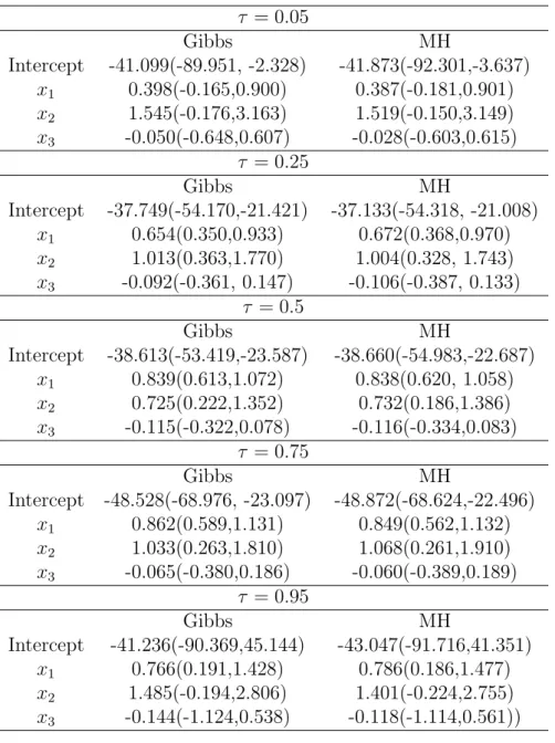
τ = {0.05,0.25,0.5,0.75,0.95}. Table 2.2 presents the posterior mean together with the 95% highest posterior density (HPD) region in parentheses for each
chain. A word of caution: the HPD intervals are conditional on the choice of like-lihood. They are presented here as a way to compare how well both algorithms explore the posterior distribution.
It can be seen from Table 2.2 that both the estimates and the HPD inter-vals are very similar across all quantiles, indicating that for small dimensional problems, Gibbs and MH perform similarly well at exploring the posterior distri-bution despite then = 21 additional parameters for the Gibbs sampler to update. The MH algorithm was run using the optimal settings recommended by Yu and Moyeed (2001).
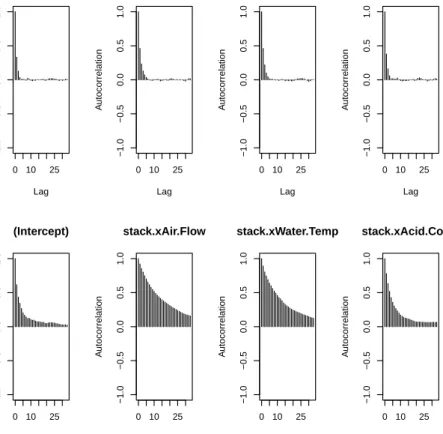
It should be noted that the Gibbs sampler for τ = 0.5 produces samples that have significantly lower autocorrelation than MH (see Figure 2.1). Whilst it is true that any MH algorithm is always likely to have higher autocorrelation than a Gibbs sampler given that all candidate values are accepted in Gibbs sampling, another factor may be that the Gibbs sampler updates the regression parameters in one block and the latent parameters in another block. In contrast, the advan-tage associated with being able to choose univariate candidate densities for MH by holding the remaining parameters constant is negated by the fact that the predictors are correlated. The correlation between water temperature and acid concentration is about 0.39, between acid concentration and air flow is 0.5 and between water temperature and air flow is 0.78. As a result, any sampler that up-dates each parameter one by one conditional on the other parameters being held fixed is less likely to be able to make large moves and fully explore the posterior distribution in a reasonable amount of time. On this basis, the Gibbs sampler is more efficient when τ = 0.5.
2.4
Bayesian Quantile Regression with Natural
Cubic Splines
Recently, Thompson et al. (2010) used the approach of Yu and Moyeed (2001) to implement non parametric Bayesian quantile regression using natural cubic
τ = 0.05 Gibbs MH Intercept -41.099(-89.951, -2.328) -41.873(-92.301,-3.637) x1 0.398(-0.165,0.900) 0.387(-0.181,0.901) x2 1.545(-0.176,3.163) 1.519(-0.150,3.149) x3 -0.050(-0.648,0.607) -0.028(-0.603,0.615) τ = 0.25 Gibbs MH Intercept -37.749(-54.170,-21.421) -37.133(-54.318, -21.008) x1 0.654(0.350,0.933) 0.672(0.368,0.970) x2 1.013(0.363,1.770) 1.004(0.328, 1.743) x3 -0.092(-0.361, 0.147) -0.106(-0.387, 0.133) τ = 0.5 Gibbs MH Intercept -38.613(-53.419,-23.587) -38.660(-54.983,-22.687) x1 0.839(0.613,1.072) 0.838(0.620, 1.058) x2 0.725(0.222,1.352) 0.732(0.186,1.386) x3 -0.115(-0.322,0.078) -0.116(-0.334,0.083) τ = 0.75 Gibbs MH Intercept -48.528(-68.976, -23.097) -48.872(-68.624,-22.496) x1 0.862(0.589,1.131) 0.849(0.562,1.132) x2 1.033(0.263,1.810) 1.068(0.261,1.910) x3 -0.065(-0.380,0.186) -0.060(-0.389,0.189) τ = 0.95 Gibbs MH Intercept -41.236(-90.369,45.144) -43.047(-91.716,41.351) x1 0.766(0.191,1.428) 0.786(0.186,1.477) x2 1.485(-0.194,2.806) 1.401(-0.224,2.755) x3 -0.144(-1.124,0.538) -0.118(-1.114,0.561))
Table 2.2: Comparison of Gibbs sampler and Metropolis-Hastings(MH). The pos-terior means were recorded together with the 95% highest pospos-terior density (HPD) intervals (in parentheses).
0 10 25 −1.0 −0.5 0.0 0.5 1.0 Lag A utocorrelation (Intercept) 0 10 25 −1.0 −0.5 0.0 0.5 1.0 Lag A utocorrelation stack.xAir.Flow 0 10 25 −1.0 −0.5 0.0 0.5 1.0 Lag A utocorrelation stack.xWater.Temp 0 10 25 −1.0 −0.5 0.0 0.5 1.0 Lag A utocorrelation stack.xAcid.Conc. 0 10 25 −1.0 −0.5 0.0 0.5 1.0 Lag A utocorrelation (Intercept) 0 10 25 −1.0 −0.5 0.0 0.5 1.0 Lag A utocorrelation stack.xAir.Flow 0 10 25 −1.0 −0.5 0.0 0.5 1.0 Lag A utocorrelation stack.xWater.Temp 0 10 25 −1.0 −0.5 0.0 0.5 1.0 Lag A utocorrelation stack.xAcid.Conc.
Figure 2.1: Stackloss data: Comparing autocorrelation of Gibbs and MH at τ = 0.5. The top row corresponds to the Gibbs sampler, the bottom row to MH with optimal settings.
splines (NCS). In this section, a Gibbs sampler designed using the same approach as the previous sections is compared to the MH algorithm used by Thompson et al. (2010). Following the authors, artificial data was simulated based on the motorcycle data obtained in an experiment to test crash helmets and discussed in Silverman (1985). This dataset is a classic example of where polynomial re-gression is inappropriate. The response variable y of the motorcycle data is a record of the head acceleration, measured in multiples of the acceleration due to gravity g. The explanatory variablexis the time, measured in milliseconds, after a simulated motorcycle accident. An artificial dataset was formed by simulating 100 observations at 30 evenly spaced time points from a normal distribution with mean equal to the value of the smoothing spline fitted to the motorcycle data at each time point and standard deviation equal to 20.
Using the notation of Green and Silverman (1994), let ti be the ordered set of
knots that are in the range of x and let gi = g(ti) denote the value of the NCS
at the knot points ti. The AL likelihood l(y|g), where g is a 30×1 vector with
elements gi, is then proportional to
Y i,j exp{−1 2|yij −gi|} Y i,j exp{−(τ −1 2)(yij−gi)}, (2.15)
where i runs from 1 to 30 and j runs from 1 to 100. The model of Thompson et al. (2010) assumes a multivariate normal prior for g,
π(g|λ)∝λn/2exp(−λ
2g
TKg). (2.16)
This choice was motivated by the fact that the log density is proportional to the roughness penalty Rabg00(x)2dx as a consequence of theorem 2.1 in Green and
Silverman (1994). The matrix K is a fixed symmetric matrix of rank 28 defined asQR−1QT. Defininghi =ti+1−ti fori= 1, . . . ,29, the matrixQis 30×28 with
entries qij, i = 1, . . . ,30, j = 2, . . . ,29, with qj−1,j = h−j−11, qjj = −h−j−11 −h
−1
j ,
qj+1,j = h−j1 for j = 2, . . . ,29 and qij = 0 for |i −j| ≥ 2. The matrix R is a
rii = 13(hi−1 +hi), i = 2, . . . ,29, ri,i+1 = ri+1,i = 16hi, i = 2, . . . ,28 and rij = 0
for |i−j| ≥ 2. The parameter λ denotes the smoothing parameter that acts as a compromise between smoothness and fidelity to the data. Finally, the model of Thompson et al. (2010) treats λ as unknown and gives it a Gamma hyperprior with parameters c0 and d0,
π(λ)∝λc0−1exp(−d0λ). (2.17)
Instead of using the random walk Metropolis within Gibbs as in Yu and Moy-eed (2001), Thompson et al. (2010) opt for an MH algorithm that updates the entire vector g in one block followed by an update forλ. The main disadvantage with this approach is the “curse of dimensionality” - to find a suitable candi-date density that performs well and gives good mixing is extremely hard in high dimensional problems.
In order to implement a Gibbs sampler, an additional 3,000 latent variables in a 30×100 matrix W need to be introduced into the model. The augmented likelihood l(y|g,W,y) is proportional to Y i,j √ wijexp{−12wij(yij −gi)2} Y i,j exp{−(τ− 1 2)(yij −gi)}. (2.18)
The final component of this augmented model is the independent and identically distributed inverse Gamma priors on each wij with parameters (1,18). Just as in
section 2, the likelihood of Thompson et al. (2010) can be recovered by marginal-ising over W.
Routine calculations reveal that the conditional posterior distribution of g is multivariate normal with precision matrix
Ω+λK (2.19)
and mean vector
(Ω+λK)−1u, (2.20)
whereΩdenotes a 30×30 diagonal matrix withΩi,i =
P100
j=1wij anduis a 30×1
vector with elements ui =
P100
Algorithm 2.3Gibbs sampler for quantile regression with natural cubic splines. Draws M burn in samples and N samples for inference.
Given: Precision matrix Kand initial values g(0).
for k = 1 to M +N do
• Sample each componentw(ijk)|g(k−1),y by sampling from the inverse
Gaus-sian distribution with shape parameter 14 and location 12|yij −g
(k−1)
i |
−1.
• Sample λ(k)|g(k−1),y from the gamma distribution with location 14 + c0
and scale 12{g(k−1)}TKg(k−1).
• Sample g(k)|W(k), λ(k),y from the multivariate normal distribution with
precision matrix
Ω(k)+λ(k)K
and mean vector
(Ω(k)+λ(k)K)−1u(k),
where Ω(g) is a 30×30 diagonal matrix with Ω(i,ig) =P100
j=1w (g)
ij and u(k) is a
30×1 vector with elements u(ik) =P100
j=1w (k)
ij yij+ 100(τ − 12). end for.
wij is inverse Gaussian with parameters (12|yij −gi|−1,14), with wij conditionally
independent of each other giveng and the datay. Finally, the conditional poste-rior for λ is gamma with parameters (14 +c0,12gTKg+d0). This Gibbs sampler
can be summarised in Algorithm (2.3)
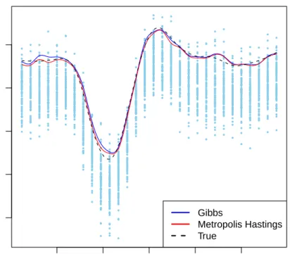
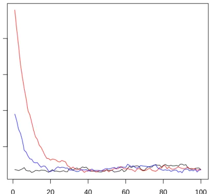
Thompson et al. (2010) analysed τ = 0.95 and ran the MH algorithm for 250,000 iterations discarding 50,000 as burn in and retaining every 10th iteration to reduce autocorrelation and for storage purposes. Figure 2.2 plots the NCS obtained by the MH algorithm and that obtained by the Gibbs sampler using 11,000 iterations, 1,000 of which were discarded as burn in.
At first glance, all seems fine. Figure 2.2 show that both the MH algorithm and the Gibbs sampler produce curves that can accurately reconstruct the true underlying curve and are very similar to each other.
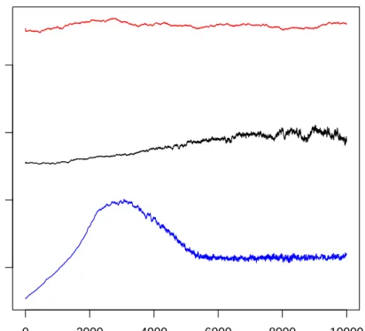
Thompson et al. (2010) assess the rate of convergence by running 3 separate MH samplers initialised with wildly different starting values. These same starting values were used to start 3 additional Gibbs samplers. Figure 2.3 shows the first 10,000 iterations of the 3 chains under MH sampling for the first knot g1. Figure
● ● ● ● ● ● ● ● ● ● ● ● ● ● ● ● ● ● ● ● ● ● ● ● ● ● ● ● ● ● ● ● ● ● ● ● ● ● ● ● ● ● ● ● ● ● ● ● ● ● ● ● ● ● ● ● ● ● ● ● ● ● ● ● ● ● ● ● ● ● ● ● ● ● ● ● ● ● ● ● ● ● ● ● ● ● ● ● ● ● ● ● ● ● ● ● ● ● ● ● ● ● ● ● ● ● ● ● ● ● ● ● ● ● ● ● ● ● ● ● ● ● ● ● ● ● ● ● ● ● ● ● ● ● ● ● ● ● ● ● ● ● ● ● ● ● ● ● ● ● ● ● ● ● ● ● ● ● ● ● ● ● ● ● ● ● ● ● ● ● ● ● ● ● ● ● ● ● ● ● ● ● ● ● ● ● ● ● ● ● ● ● ● ● ● ● ● ● ● ● ● ● ● ● ● ● ● ● ● ● ● ● ● ● ● ● ● ● ● ● ● ● ● ● ● ● ● ● ● ● ● ● ● ● ● ● ● ● ● ● ● ● ● ● ● ● ● ● ● ● ● ● ● ● ● ● ● ● ● ● ● ● ● ● ● ● ● ● ● ● ● ● ● ● ● ● ● ● ● ● ● ● ● ● ● ● ● ● ● ● ● ● ● ● ● ● ● ● ● ● ● ● ● ● ● ● ● ● ● ● ● ● ● ● ● ● ● ● ● ● ● ● ● ● ● ● ● ● ● ● ● ● ● ● ● ● ● ● ● ● ● ● ● ● ● ● ● ● ● ● ● ● ● ● ● ● ● ● ● ● ● ● ● ● ● ● ● ● ● ● ● ● ● ● ● ● ● ● ● ● ● ● ● ● ● ● ● ● ● ● ● ● ● ● ● ● ● ● ● ● ● ● ● ● ● ● ● ● ● ● ● ● ● ● ● ● ● ● ● ● ● ● ● ● ● ● ● ● ● ● ● ● ● ● ● ● ● ● ● ● ● ● ● ● ● ● ● ● ● ● ● ● ● ● ● ● ● ● ● ● ● ● ● ● ● ● ● ● ● ● ● ● ● ● ● ● ● ● ● ● ● ● ● ● ● ● ● ● ● ● ● ● ● ● ● ● ● ● ● ● ● ● ● ● ● ● ● ● ● ● ● ● ● ● ● ● ● ● ● ● ● ● ● ● ● ● ● ● ● ● ● ● ● ● ● ● ● ● ● ● ● ● ● ● ● ● ● ● ● ● ● ● ● ● ● ● ● ● ● ● ● ● ● ● ● ● ● ● ● ● ● ● ● ● ● ● ● ● ● ● ● ● ● ● ● ● ● ● ● ● ● ● ● ● ● ● ● ● ● ● ● ● ● ● ● ● ● ● ● ● ● ● ● ● ● ● ● ● ● ● ● ● ● ● ● ● ● ● ● ● ● ● ● ● ● ● ● ● ● ● ● ● ● ● ● ● ● ● ● ● ● ● ● ● ● ● ● ● ● ● ● ● ● ● ● ● ● ● ● ● ● ● ● ● ● ● ● ● ● ● ● ● ● ● ● ● ● ● ● ● ● ● ● ● ● ● ● ● ● ● ● ● ● ● ● ● ● ● ● ● ● ● ● ● ● ● ● ● ● ● ● ● ● ● ● ● ● ● ● ● ● ● ● ● ● ● ● ● ● ● ● ● ● ● ● ● ● ● ● ● ● ● ● ● ● ● ● ● ● ● ● ● ● ● ● ● ● ● ● ● ● ● ● ● ● ● ● ● ● ● ● ● ● ● ● ● ● ● ● ● ● ● ● ● ● ● ● ● ● ● ● ● ● ● ● ● ● ● ● ● ● ● ● ● ● ● ● ● ● ● ● ● ● ● ● ● ● ● ● ● ● ● ● ● ● ● ● ● ● ● ● ● ● ● ● ● ● ● ● ● ● ● ● ● ● ● ● ● ● ● ● ● ● ● ● ● ● ● ● ● ● ● ● ● ● ● ● ● ● ● ● ● ● ● ● ● ● ● ● ● ● ● ● ● ● ● ● ● ● ● ● ● ● ● ● ● ● ● ● ● ● ● ● ● ● ● ● ● ● ● ● ● ● ● ● ● ● ● ● ● ● ● ● ● ● ● ● ● ● ● ● ● ● ● ● ● ● ● ● ● ● ● ● ● ● ● ● ● ● ● ● ● ● ● ● ● ● ● ● ● ● ● ● ● ● ● ● ● ● ● ● ● ● ● ● ● ● ● ● ● ● ● ● ● ● ● ● ● ● ● ● ● ● ● ● ● ● ● ● ● ● ● ● ● ● ● ● ● ● ● ● ● ● ● ● ● ● ● ● ● ● ● ● ● ● ● ● ● ● ● ● ● ● ● ● ● ● ● ● ● ● ● ● ● ● ● ● ● ● ● ● ● ● ● ● ● ● ● ● ● ● ● ● ● ● ● ● ● ● ● ● ● ● ● ● ● ● ● ● ● ● ● ● ● ● ● ● ● ● ● ● ● ● ● ● ● ● ● ● ● ● ● ● ● ● ● ● ● ● ● ● ● ● ● ● ● ● ● ● ● ● ● ● ● ● ● ● ● ● ● ● ● ● ● ● ● ● ● ● ● ● ● ● ● ● ● ● ● ● ● ● ● ● ● ● ● ● ● ● ● ● ● ● ● ● ● ● ● ● ● ● ● ● ● ● ● ● ● ● ● ● ● ● ● ● ● ● ● ● ● ● ● ● ● ● ● ● ● ● ● ● ● ● ● ● ● ● ● ● ● ● ● ● ● ● ● ● ● ● ● ● ● ● ● ● ● ● ● ● ● ● ● ● ● ● ● ● ● ● ● ● ● ● ● ● ● ● ● ● ● ● ● ● ● ● ● ● ● ● ● ● ● ● ● ● ● ● ● ● ● ● ● ● ● ● ● ● ● ● ● ● ● ● ● ● ● ● ● ● ● ● ● ● ● ● ● ● ● ● ● ● ● ● ● ● ● ● ● ● ● ● ● ● ● ● ● ● ● ● ● ● ● ● ● ● ● ● ● ● ● ● ● ● ● ● ● ● ● ● ● ● ● ● ● ● ● ● ● ● ● ● ● ● ● ● ● ● ● ● ● ● ● ● ● ● ● ● ● ● ● ● ● ● ● ● ● ● ● ● ● ● ● ● ● ● ● ● ● ● ● ● ● ● ● ● ● ● ● ● ● ● ● ● ● ● ● ● ● ● ● ● ● ● ● ● ● ● ● ● ● ● ● ● ● ● ● ● ● ● ● ● ● ● ● ● ● ● ● ● ● ● ● ● ● ● ● ● ● ● ● ● ● ● ● ● ● ● ● ● ● ● ● ● ● ● ● ● ● ● ● ● ● ● ● ● ● ● ● ● ● ● ● ● ● ● ● ● ● ● ● ● ● ● ● ● ● ● ● ● ● ● ● ● ● ● ● ● ● ● ● ● ● ● ● ● ● ● ● ● ● ● ● ● ● ● ● ● ● ● ● ● ● ● ● ● ● ● ● ● ● ● ● ● ● ● ● ● ● ● ● ● ● ● ● ● ● ● ● ● ● ● ● ● ● ● ● ● ● ● ● ● ● ● ● ● ● ● ● ● ● ● ● ● ● ● ● ● ● ● ● ● ● ● ● ● ● ● ● ● ● ● ● ● ● ● ● ● ● ● ● ● ● ● ● ● ● ● ● ● ● ● ● ● ● ● ● ● ● ● ● ● ● ● ● ● ● ● ● ● ● ● ● ● ● ● ● ● ● ● ● ● ● ● ● ● ● ● ● ● ● ● ● ● ● ● ● ● ● ● ● ● ● ● ● ● ● ● ● ● ● ● ● ● ● ● ● ● ● ● ● ● ● ● ● ● ● ● ● ● ● ● ● ● ● ● ● ● ● ● ● ● ● ● ● ● ● ● ● ● ● ● ● ● ● ● ● ● ● ● ● ● ● ● ● ● ● ● ● ● ● ● ● ● ● ● ● ● ● ● ● ● ● ● ● ● ● ● ● ● ● ● ● ● ● ● ● ● ● ● ● ● ● ● ● ● ● ● ● ● ● ● ● ● ● ● ● ● ● ● ● ● ● ● ● ● ● ● ● ● ● ● ● ● ● ● ● ● ● ● ● ● ● ● ● ● ● ● ● ● ● ● ● ● ● ● ● ● ● ● ● ● ● ● ● ● ● ● ● ● ● ● ● ● ● ● ● ● ● ● ● ● ● ● ● ● ● ● ● ● ● ● ● ● ● ● ● ● ● ● ● ● ● ● ● ● ● ● ● ● ● ● ● ● ● ● ● ● ● ● ● ● ● ● ● ● ● ● ● ● ● ● ● ● ● ● ● ● ● ● ● ● ● ● ● ● ● ● ● ● ● ● ● ● ● ● ● ● ● ● ● ● ● ● ● ● ● ● ● ● ● ● ● ● ● ● ● ● ● ● ● ● ● ● ● ● ● ● ● ● ● ● ● ● ● ● ● ● ● ● ● ● ● ● ● ● ● ● ● ● ● ● ● ● ● ● ● ● ● ● ● ● ● ● ● ● ● ● ● ● ● ● ● ● ● ● ● ● ● ● ● ● ● ● ● ● ● ● ● ● ● ● ● ● ● ● ● ● ● ● ● ● ● ● ● ● ● ● ● ● ● ● ● ● ● ● ● ● ● ● ● ● ● ● ● ● ● ● ● ● ● ● ● ● ● ● ● ● ● ● ● ● ● ● ● ● ● ● ● ● ● ● ● ● ● ● ● ● ● ● ● ● ● ● ● ● ● ● ● ● ● ● ● ● ● ● ● ● ● ● ● ● ● ● ● ● ● ● ● ● ● ● ● ● ● ● ● ● ● ● ● ● ● ● ● ● ● ● ● ● ● ● ● ● ● ● ● ● ● ● ● ● ● ● ● ● ● ● ● ● ● ● ● ● ● ● ● ● ● ● ● ● ● ● ● ● ● ● ● ● ● ● ● ● ● ● ● ● ● ● ● ● ● ● ● ● ● ● ● ● ● ● ● ● ● ● ● ● ● ● ● ● ● ● ● ● ● ● ● ● ● ● ● ● ● ● ● ● ● ● ● ● ● ● ● ● ● ● ● ● ● ● ● ● ● ● ● ● ● ● ● ● ● ● ● ● ● ● ● ● ● ● ● ● ● ● ● ● ● ● ● ● ● ● ● ● ● ● ● ● ● ● ● ● ● ● ● ● ● ● ● ● ● ● ● ● ● ● ● ● ● ● ● ● ● ● ● ● ● ● ● ● ● ● ● ● ● ● ● ● ● ● ● ● ● ● ● ● ● ● ● ● ● ● ● ● ● ● ● ● ● ● ● ● ● ● ● ● ● ● ● ● ● ● ● ● ● ● ● ● ● ● ● ● ● ● ● ● ● ● ● ● ● ● ● ● ● ● ● ● ● ● ● ● ● ● ● ● ● ● ● ● ● ● ● ● ● ● ● ● ● ● ● ● ● ● ● ● ● ● ● ● ● ● ● ● ● ● ● ● ● ● ● ● ● ● ● ● ● ● ● ● ● ● ● ● ● ● ● ● ● ● ● ● ● ● ● ● ● ● ● ● ● ● ● ● ● ● ● ● ● ● ● ● ● ● ● ● ● ● ● ● ● ● ● ● ● ● ● ● ● ● ● ● ● ● ● ● ● ● ● ● ● ● ● ● ● ● ● ● ● ● ● ● ● ● ● ● ● ● ● ● ● ● ● ● ● ● ● ● ● ● ● ● ● ● ● ● ● ● ● ● ● ● ● ● ● ● ● ● ● ● ● ● ● ● ● ● ● ● ● ● ● ● ● ● ● ● ● ● ● ● ● ● ● ● ● ● ● ● ● ● ● ● ● ● ● ● ● ● ● ● ● ● ● ● ● ● ● ● ● ● ● ● ● ● ● ● ● ● ● ● ● ● ● ● ● ● ● ● ● ● ● ● ● ● ● ● ● ● ● ● ● ● ● ● ● ● ● ● ● ● ● ● ● ● ● ● ● ● ● ● ● ● ● ● ● ● ● ● ● ● ● ● ● ● ● ● ● ● ● ● ● ● ● ● ● ● ● ● ● ● ● ● ● ● ● ● ● ● ● ● ● ● ● ● ● ● ● ● ● ● ● ● ● ● ● ● ● ● ● ● ● ● ● ● ● ● ● ● ● ● ● ● ● ● ● ● ● ● ● ● ● ● ● ● ● ● ● ● ● ● ● ● ● ● ● ● ● ● ● ● ● ● ● ● ● ● ● ● ● ● ● ● ● ● ● ● ● ● ● ● ● ● ● ● ● ● ● ● ● ● ● ● ● ● ● ● ● ● ● ● ● ● ● ● ● ● ● ● ● ● ● ● ● ● ● ● ● ● ● ● ● ● ● ● ● ● ● ● ● ● ● ● ● ● ● ● ● ● ● ● ● ● ● ● ● ● ● ● ● ● ● ● ● ● ● ● ● ● ● ● ● ● ● ● ● ● ● ● ● ● ● ● ● ● ● ● ● ● ● ● ● ● ● ● ● ● ● ● ● ● ● ● ● ● ● ● ● ● ● ● ● ● ● ● ● ● ● ● ● ● ● ● ● ● ● ● ● ● ● ● ● ● ● ● ● ● ● ● ● ● ● ● ● ● ● ● ● ● ● ● ● ● ● ● ● ● ● ● ● ● ● ● ● ● ● ● ● ● ● ● ● ● ● ● ● ● ● ● ● ● ● ● ● ● ● ● ● ● ● ● ● ● ● ● ● ● ● ● ● ● ● ● ● ● ● ● ● ● ● ● ● ● ● ● ● ● ● ● ● 10 20 30 40 50 −150 −100 −50 0 50
Time (milliseconds after impact)
Sim ulated Acceler ation (m ultiples of g) Gibbs Metropolis Hastings True
Figure 2.2: Bayesian nonparametric regression using NCS for τ = 0.95. The blue curve is obtained from our Gibbs sampler, the red curve is obtained from MH. The dashed black curve is the true underlying curve.
Iteration 0 2000 4000 6000 8000 10000 −50 0 50 100
Figure 2.3: Plot of the first 10,000 iterations of the Metropolis Hastings chains, plotted for g1.
Iteration 0 20 40 60 80 100 40 60 80 100
The disadvantage of the MH algorithm is immediately evident from Figure 2.3 and Figure 2.4. The chains obtained using MH have not forgotten their starting values after 10,000 iterations. In fact, even after running the 3 chains for the full 250,000 iterations, discarding the first 50,000 iterations and thinning, the posterior mean forg(not shown here) was different for each chain. In contrast, observe that the 3 chains obtained by running the Gibbs sampler converged on each other very quickly, despite having 3,000 additional parameters to update. This is likely to be due to the fact that the Gibbs sampler blocks all 3,000 latent parameters together, thus reducing the negative effect alluded to in Liu et al. (1994) of having 3,000 additional parameters to update. Running the Gibbs samplers with 3 different starting values each for 11,000 iterations discarding the first 1,000 gave values of the Gelman-Rubin (Gelman and Rubin, 1992) diagnostic of between 1.000 and 1.013. The posterior mean for g was virtually identical for each chain. These results demonstrate the apparent superiority of the Gibbs sampler in these higher dimensional cases.
The posterior mean for λwas about 0.03. This value of λindicates that those curves that fit the data well but are fairly “wiggly” are preferred for this example.
2.5
Summary
This chapter has provided the framework for allowing Bayesian parameter estima-tion to be implemented on more complex quantile regression models in a relatively straightforward manner. Despite the observations by Liu et al. (1994) suggesting that adding latent variables will slow convergence, no evidence of this has been observed. In fact, it is particularly evident when analysing the nonparametric quantile regression model with natural cubic splines that the Gibbs sampler is a much more efficient MCMC sampler. Although it was possible to accurately reconstruct the underlying curve using both the Gibbs sampler and the MH algo-rithm of Thompson et al. (2010), the MH sampler requires good prior knowledge about starting values whereas the Gibbs sampler appears not to be affected by
the starting values. These observations could be due to a number of factors, most notably that it is extremely difficult to choose a sensible proposal density in high dimensional problems and that the Gibbs sampler can update the latent param-eters jointly whilst sampling directly from the conditional π(g|W, λ,y).
Chapter 3
An Application in Epidemiology:
Is Maternal Cotinine a Better
Predictor of Low Birthweight
Infants than the Reported
Number of Cigarettes?
3.1
Introduction and Method
Many previous studies analysing infant birthweight have analysed how various factors have affected average birthweight (Peacock et al. (1998) and references therein). However, as Abrevaya and Dahl (2008) have pointed out, there are greater costs associated with low birthweight (LBW) infants. Moreover, it has been observed that it is more likely for LBW infants to have a greater mortality rate, in addition to likely problems in development and education (LBW infants are more likely to repeat a year) and ultimately, are more likely to be unemployed (see Abrevaya and Dahl (2008) and references therein).
The aim of this study is to use quantile regression on the St George’s Birth-weight study data to explore whether results presented in Peacock et al. (1998) hold for the lower quantiles of the conditional distribution. In using quantile regression, it will be possible to analyse the median and hence investigate the robustness of the original results.
be required. The Bayesian approach to comparing competing models is to use the Bayes factor, defined as π(y|Model 1)/π(y|Model 2). If there is no reason to sus-pect that model 1 is more likely to have generated the data than model 2a priori, then the Bayes factor is equivalent to the posterior oddsπ(Model 1|y)/π(Model 2|y). Using the Bayesian approach compares the likelihoods averaged over the param-eters of the models rather than the maximum likelihoods used in frequentist statistics. The averaging of the likelihood over the parameters naturally penalises a model for the size of its parameter space, hence offering a model comparison tool that trades off goodness of fit against model complexity.
Combined with the AL likelihood (1.9), the prior
β|λ∼N(0,Λ−1) (3.1)
is used throughout this chapter. Here,λis a (p+ 1)×1 vector of hyperparameters
λj and Λ is a (p+ 1)×(p+ 1) diagonal matrix with Λj,j =λj. To let the data
influence the results as much as possible, λj can be set to a constant cand then
lettingctend to 0. This results in a joint improper uniform prior forβ. However, this improper prior leads to indeterminate Bayes factors. A compromise between robustness and avoiding indeterminate Bayes factors is to give each λj a gamma
hyperprior with parameters (12,12). Marginalised over λ, this gives a product of standard Cauchy(0,1) distributions as the joint prior on β. These have more probability mass in the tails than the normal.
Just as before, data augmentation plays a key role in designing more efficient Gibbs samplers. Under the improper prior on β, the resulting Gibbs sampler is the same as that in Chapter 2 using b0 =0 and B0 = cI and c → 0. With the Cauchy priors, an additional update of each of the latent λj is required, similar
in spirit to the Gibbs sampler for NCS. These can be updated independently of each other and are exponentially distributed with rate parameter 12(1 +βj2). The procedure is described in Algorithm 3.1.
Algorithm 3.1 Gibbs sampler for augmented quantile regression model under independent Cauchy priors on β. Draws M burn in samples followed by an addi-tional N samples for inference.
Given: Initial values β(0).
for k = 1 to M +N do
• Sample w(k)|β(k−1),y by sampling the ith component of w (i = 1, . . . , n) from the inverse Gaussian distribution with shape parameter 14 and location
1
2|yi−xi
Tβ(k−1)|−1.
• Update each component ofλ(k) from an exponential distribution with rate
1
2{1 +{β (k−1)
j }2}.
• Sample β(k)|w(k),λ(k)
,y from the multivariate normal distribution with precision matrix
XTW(k)X+Λ(k)
and mean vector
(XTW(k)X+Λ(k))−1(XTW(k)y+ (τ − 1 2)X
T1,
where W(k) and Λ(k) are diagonal matrices. Each element ofw(k) forms the
diagonal of W(k) and the diagonal elements of Λ(k) are {λ(k)
j }. end for.
convergence were found after 1,000 iterations. Once these first 1,000 iterations had been discarded, inference was based on 10,000 further iterations.
For the analysis under the Cauchy priors, the Bayes factors were calculated from the samples using Chib’s method (Chib, 1995). This approach uses a rear-rangement of Bayes theorem. In this case, conditional on a model, Bayes theorem gives
l(y) = l(y|β)π(β)
π(β|y) . (3.2)
Equation (3.2) remains true if β is substituted by it’s posterior mean ˆβ. Thus, an algorithm can be developed making use of the Gibbs samples to calculate an approximate marginal for y conditional on a fixed model. This is summarised in Algorithm 3.2.
Algorithm 3.2 can be repeated with other models to form approximate Bayes factors. The most computationally intense part in this calculation is evaluating the posterior marginal density ordinate π( ˆβ|y), which requires additional iterations from the Gibbs sampler to get a good approximation.
Algorithm 3.2 Chib’s method for calculating approximate marginal likelihood
l(y).
Given: Gibbs sample obtained using Algorithm 3.1.
• From the Gibbs sample, discard the burn in and average over the remaining samples to produce an estimate of the marginal posterior mean ˆβ.
• Evaluate l(y|βˆ) and π( ˆβ). These are both available in closed form, the first being the AL likelihood and the second a product of Cauchy density ordinates.
• Using the current state of the Gibbs sampler, obtain N addition samples using Algorithm 3.1. Record the density ordinate at each sampled value of w
and λ,π( ˆβ|w(k),λ(k)) for k=M +N + 1, . . . , M + 2N. •Approximate π( ˆβ|y) with ˆ π( ˆβ|y) = 1 N M+2N X k=M+N+1 π( ˆβ|w(k),λ(k)). (3.3)
•Plug these values into (3.2) to obtain an approximation of ˆπ(y).
3.2
Results
The original research by Peacock et al. (1998), investigated two main questions, namely i) whether maternal serum cotinine level, a metabolite of nicotine, is a better predictor of infant’s birthweight than the reported number of cigarettes smoked by the mother and ii) what the effect of passive smoke exposure on birth-weight among women who do not smoke is. This dataset was analysed again to investigate relationships at the median and the lower tails of the conditional birthweight distribution. Following the original analysis, quantile regression was used with the response variable being adjusted birthweight (birthweight adjusted for gestational age, maternal height, sex of infant and parity, where the adjusted birthweight is effectively a ratio of observed to expected values and can be inter-preted as percentage differences from expected values (Bland et al., 1990)). The models investigated included one or more of the following covariates:
• cotinine
• nicotine yield of cigarette
For each model, data recorded at three time points was analysed: at booking clinic (approximately 14 weeks gestation), at 28 weeks gestation and at 36 weeks gestation. The difference between cotinine measured at each of the different time points was also modelled to help identify whether a change in smoking habit has an effect on the adjusted birthweight. As a final anaysis, data for women who were not active smokers (determined by a cotinine measurement level less than 15ng/ml) were analysed to see if there are any effects of passive smoke on the adjusted birthweight.
A quick glance at the scatterplot of cotinine level at booking against adjusted birthweight (Figure 3.1) suggests that the linear regression model used by Peacock et al. (1998) seems sensible for the majority of conditional quantiles of the adjusted birthweight distribution. Here, the term “linear” is referring both to regression linear in the parameters and a regression equation that is a straight line. The plots look similar for cotinine measured at 28 weeks and 36 weeks so are not presented here. This analysis is therefore based on simple linear quantile regression.
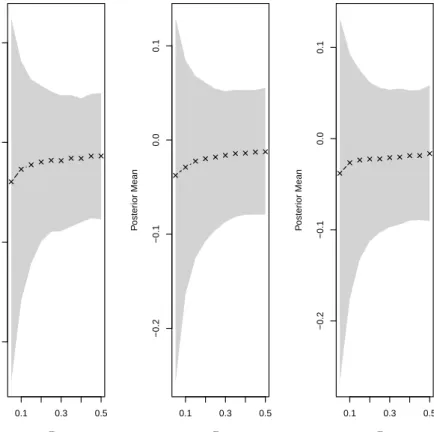
Figure 3.2 plots the posterior mean cotinine as a function of τ for τ ∈ {0.05,0.1, . . . ,0.45,0.5}. The shaded region is the associated 95% HPD inter-val. Just as in the previous chapter, the HPD interval should be interpreted with caution as it is subject to the likelihood representing the true underlying data generating mechanism, something that is never assumed in the analysis. It does however serve as a rough guide for exploratory analysis.
Figure 3.2 shows that at all 3 timepoints the posterior mean birthweight grad-ually decreases until τ = 0.15, then it appears to decreases significantly faster as
τ gets smaller. The implications are that smoking has a much larger effect on the more severely underweight infants.
Turning to the question of whether cotinine is a better predictor than the
50 100 150 200 250 300 350
0.6
0.8