Superelement User's
Guide
Proprietary & Restricted Rights Notice . . . 7 Introduction and Fundamentals . . . 1-1
Why Use Superelements? . . . 1-2 Reduced Cost . . . 1-3 Quicker Turnaround . . . 1-3 Reduced Risk . . . 1-3 Large Problem Capabilities . . . 1-3 Partitioned Input and Output . . . 1-3 Security . . . 1-4 Fundamentals of Superelement Analysis . . . 1-4 Partitioned Solutions . . . 1-6 Example to Show the Use of Superelements in Static Analysis . . . 1-8 Conventional Analysis . . . 1-9 Superelement Analysis . . . 1-11 Superelement 1 . . . 1-12 Superelement 2 . . . 1-15 Residual Structure . . . 1-16
How to Define a Superelement . . . 2-1
Defining a Superelement Using Partitioned Bulk Data . . . 2-2 Defining PARTs . . . 2-2 The Bulk Data Section Using PARTs . . . 2-3 Format of the Input File When PARTs Are Used . . . 2-3 Automatically Connecting PARTs to Other Components of the Model . . . 2-12 Constraints on Connecting Points . . . 2-12 Manually Defining Exterior Points for a PART . . . 2-17 Moving and/or Rotating PARTs . . . 2-17 Defining Superelements in the Main Bulk Data Section . . . 2-22 Superelement Definition . . . 2-22 Interior Versus Exterior Points . . . 2-23 Bulk Data Partitioning . . . 2-23 Example of Bulk Data Partitioning . . . 2-24 The Superelement MAP - SEMAP . . . 2-28 Defining External Superelements . . . 2-30 External Superelement Procedure Overview . . . 2-30 NX Nastran Input File Requirements for Component Solutions . . . 2-32 NX Nastran Input File Requirements for System Solutions . . . 2-35 External Superelement Loads . . . 2-36 External Superelement Examples . . . 2-37
Introduction . . . 3-2 Simple Input for Single-Level Analysis . . . 3-2 Single-Level Analysis Using Main Bulk Data Superelements . . . 3-3 Example of Single-Level Analysis . . . 3-3 Quick Review . . . 3-6 Single-Level Analysis When PARTs Are Present . . . 3-7
Loads, Constraints, and Case Control in Static Analysis . . . 4-1
Introduction . . . 4-2 Loads in Static Analysis . . . 4-2 Thermal Loadings in Superelement Analysis . . . 4-3 Boundary Conditions . . . 4-4 Single-Point Constraints in Superelement Analysis . . . 4-4 MPCs and R-Type Elements in the Main Bulk Data Section . . . 4-5 Case Control in Superelement Analysis . . . 4-7 The SUPER Command-Case Control Partitioning . . . 4-8 Conventional Case Control . . . 4-9 Condensed Case Control . . . 4-9 Superelement Case Control . . . 4-10 One Loading Condition—Expanded Case Control . . . 4-10 Parameters in the Case Control Section . . . 4-18
Inertia Relief Analysis Using Superelements . . . 5-1
Introduction . . . 5-2 The Concept of Inertia Relief . . . 5-2 Interface for Inertia Relief Using Superelements . . . 5-2 Example of Inertia Relief Using Superelements . . . 5-3 Selected Output from inrel2.f06 . . . 5-9
Multiple Loadings in Static Analysis . . . 6-1
Introduction . . . 6-2 How Case Control is Internally Partitioned and Used . . . 6-2 Examples for Multiple Loading Conditions . . . 6-2
Multilevel Superelement Analysis . . . 7-1
The Concept of Multilevel Analysis . . . 7-2 Comparison of Single- and Multilevel Analysis . . . 7-2 Single-Level Analysis . . . 7-2 Multilevel Analysis . . . 7-6 User Interface for Multilevel Superelements . . . 7-18 Multilevel Processing When the Model is Main Bulk Data Only . . . 7-18 Automatic Creation of the Processing Tree . . . 7-18 Manual Definition of the Processing Tree for a Model Defined in the Main Bulk Data Section Only
. . . 7-19 Multilevel Processing When the Model Uses PARTs . . . 7-20 Example: Multilevel Problem Solved by Hand . . . 7-20 SUPERELEMENT 2 . . . 7-23 Residual Structure . . . 7-24
Examples of Multilevel Superelements . . . 7-28 Input File multi1.dat-Multilevel Superelements Using Main Bulk Data Only . . . 7-30 Input File seset.mult . . . 7-31 Input File multi2.dat-Multilevel Superelements Using PARTs . . . 7-32
Output in Superelement Static Analysis . . . 8-1
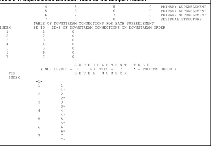
Sorted Bulk Data for PARTs . . . 8-2 Boundary Grid Search Output for PARTs . . . 8-3 Superelement Definition Table . . . 8-4
Introduction to Superelements in Dynamic Analysis . . . 9-1
Description of Dynamic Reduction Procedures . . . 9-2 Reduction Methods Used for Superelements . . . 9-3 Static Condensation (Guyan Reduction) . . . 9-3 Dynamic Reduction . . . 9-4 Fixed-Boundary Dynamic Reduction . . . 9-7 Performing Data Recovery for Superelement 2 . . . 9-18 Repeating the Same Process for Superelement 1 . . . 9-19 Free-Free Dynamic Reduction . . . 9-19 Mixed-Boundary Dynamic Reduction . . . 9-20 CMS with Exterior DOF in the C- and/or R-SET . . . 9-20
Input and Output for Dynamic Reduction . . . 10-1
Case Control for Dynamic Reduction . . . 10-2 Case Control for Dynamic Reduction . . . 10-2 Single-Level Dynamic Reduction . . . 10-4
Bulk Data Entries for Single-Level Dynamic Reduction of Main Bulk Data Superelements
. . . 10-4 Samples of Single-Level Dynamic Reduction for Main Bulk Data Superelements . . . 10-6 File cantbeam.dat - Input Model for the Examples . . . 10-6 File seg10_a.dat - Static Reduction of the Superelements . . . 10-7 File seg10_b1.dat - Fixed Boundary CMS of the Superelements . . . 10-8 File seg10-c1 - Free-Free CMS of the Superelements . . . 10-9 File seg10_d1.dat - Mixed Boundary CMS . . . 10-11 Bulk Data Entries for Single-Level Dynamic Reduction of PARTs . . . 10-13 Samples for Single-Level Dynamic Reduction Using PARTs . . . 10-14 File cantp1.dat - Bulk Data for PART 1 . . . 10-15 File cantp2.dat - Bulk Data for PART 2 . . . 10-15 File seg10p_a.dat - Static Reduction Using PARTs . . . 10-16 File seg10p_b1.dat - Fixed Boundary CMS Using PARTs . . . 10-17 File seg10p_c1.dat - Free-Free CMS Using PARTs . . . 10-20 File seg10p_d1.dat - Mixed-Boundary CMS Using PARTs . . . 10-23 Multilevel Dynamic Reduction . . . 10-24 Bulk Data Entries for Multilevel Dynamic Reduction . . . 10-24 Multilevel Dynamic Reduction for a Model With No PARTs . . . 10-25 Bulk Data Entries for Multilevel Dynamic Reduction When PART Superelements Exist . . 10-32 Sample of Multilevel CMS Using PARTs . . . 10-34
Dynamic Loading on Superelements . . . 11-1
Case Control Used to Define Dynamic Loadings on Superelements using LOADSET -LSEQ . . 11-2 LOADSET = i . . . 11-2 Bulk Data . . . 11-2 Example Demonstrating Dynamic Loads on Superelements . . . 11-3 Dynamic Loadings Applied on PARTs . . . 11-7
© 2014 Siemens Product Lifecycle Management Software Inc. All Rights Reserved.
This software and related documentation are proprietary to Siemens Product Lifecycle Management Software Inc. Siemens and the Siemens logo are registered trademarks of Siemens AG. NX is a trademark or registered trademark of Siemens Product Lifecycle Management Software Inc. or its subsidiaries in the United States and in other countries.
NASTRAN is a registered trademark of the National Aeronautics and Space Administration. NX Nastran is an enhanced proprietary version developed and maintained by Siemens Product Lifecycle Management Software Inc.
MSC is a registered trademark of MSC.Software Corporation. MSC.Nastran and MSC.Patran are trademarks of MSC.Software Corporation.
All other trademarks are the property of their respective owners. TAUCS Copyright and License
TAUCS Version 2.0, November 29, 2001. Copyright (c) 2001, 2002, 2003 by Sivan Toledo, Tel-Aviv University, [email protected]. All Rights Reserved.
TAUCS License:
Your use or distribution of TAUCS or any derivative code implies that you agree to this License. THIS MATERIAL IS PROVIDED AS IS, WITH ABSOLUTELY NO WARRANTY EXPRESSED OR IMPLIED. ANY USE IS AT YOUR OWN RISK.
Permission is hereby granted to use or copy this program, provided that the Copyright, this License, and the Availability of the original version is retained on all copies. User documentation of any code that uses this code or any derivative code must cite the Copyright, this License, the Availability note, and "Used by permission." If this code or any derivative code is accessible from within MATLAB, then typing "help taucs" must cite the Copyright, and "type taucs" must also cite this License and the Availability note. Permission to modify the code and to distribute modified code is granted, provided the Copyright, this License, and the Availability note are retained, and a notice that the code was modified is included. This software is provided to you free of charge.
Availability (TAUCS)
As of version 2.1, we distribute the code in 4 formats: zip and tarred-gzipped (tgz), with or without binaries for external libraries. The bundled external libraries should allow you to build the test programs on Linux, Windows, and MacOS X without installing additional software. We recommend that you download the full distributions, and then perhaps replace the bundled libraries by higher performance ones (e.g., with a BLAS library that is specifically optimized for your machine). If you want to conserve bandwidth and you want to install the required libraries yourself, download the lean distributions. The zip and tgz files are identical, except that on Linux, Unix, and MacOS, unpacking the tgz file ensures that the configure script is marked as executable (unpack with tar zxvpf), otherwise you will have to change its permissions manually.
• Why Use Superelements?
• Fundamentals of Superelement Analysis
• Partitioned Solutions
In finite element analysis, demand for computer resources will always exceed existing capabilities. In the early days of computers, when engineers were solving 3 x 3 problems by hand, computers were able to handle problems as large as 11 x 11. Once engineers discovered this ability, the size of engineering problems quickly grew to exceed the capacity of the existing systems. This process has repeated itself time and time again. Today modern computers are capable of solving problems involving more than 1,000,000 equations with 1,000,000 unknowns, which is still not enough to satisfy the needs of many engineers.
This limit on hardware resources, combined with budget restrictions (large runs can be
time-consuming and expensive), limits the ability of engineers to solve large, complicated problems. A solution to these problems, in terms of both hardware and budget, is the use of superelements in NX Nastran.
Using superelements, you can not only analyze large models (including those that exceed the capacity of your hardware), but can become more efficient in performing the analysis, thus allowing more design cycles or iterations in the analysis.
The principle used in superelement analysis is often referred to as substructuring. That is, the model is divided into a series of components (superelements), each of which is processed independently, resulting in a set of reduced matrices that describe the behavior of the superelement as seen by the rest of the structure. These reduced matrices for the individual superelements are combined to form an assembly (or residual) solution. The results of the assembly solution are then used to perform data recovery (calculation of displacements, stresses, etc.) for the superelements.
In static analysis the theory used in superelement processing is exact. In dynamics the reduction of the stiffness is exact, but approximations occur during the reduction of the mass and damping matrices. These approximations may be improved by using a method called component modal synthesis, which is described in“Introduction to Superelements in Dynamic Analysis”.
This user’s guide is intended to be tutorial in format: Emphasis is on how to use superelements, not on the theory of superelements. Sufficient theory is presented for those who wish to understand the operations. Hand-solved samples are included to help you understand the operations involved when superelements are used. Sample NX Nastran input files and selected output are also presented at appropriate points for clarity.
This guide is arranged so that an experienced finite element analyst can start at the beginning and read only the information applicable to the type of analysis desired. Overall information on superelements is presented first, followed by information for static analysis, followed by dynamics and other features. You should read this guide from the beginning, because much of the information presented in the section on statics is applicable in subsequent sections (similar to engineering itself); however, an engineer should be able to read the applicable sections without having to read unnecessary information.
1.1
Why Use Superelements?
Efficiency is the primary reason to use superelements. A finite element model is rarely analyzed only once. Often the model is modified and re-analyzed time and time again. Without using superelements, each analysis can cost the price of a complete solution. Doing this can deplete a budget in a short time. What follows is a partial list of the advantages of superelements.
Reduced Cost
Instead of solving the entire model each time, superelements offer the advantage of incremental processing. On restarts, this advantage is magnified by the need to process only the parts of the structure directly affected by the change. This means that if you think ahead when defining superelements, you can achieve performance improvements on the order of anywhere from 2 to 30 times faster than non-superelement methods. The use of split databases allows control of disk usage and reduces the computer resource requirements for individual runs without sacrificing the accuracy of the results obtained.
Quicker Turnaround
Because superelements can be processed individually with less computer resources required than a complete, non-superelement solution, it is often possible to submit individual superelement processing runs usingfastqueues (or even on different computers), rather than waiting and running the complete problem at once using an overnight queue.
Reduced Risk
Processing a model without using superelements is an all-or-nothing proposition. If an error occurs, the entire model must be processed again once the error is corrected. With superelements, each superelement need be processed only once, unless a change requires reprocessing the superelement. If an error occurs during processing, only the affected superelement and the residual structure (final superelement to be processed) need be reprocessed. The superelements that did not have an error do not need to be processed again until a change is made to those superelements.
Large Problem Capabilities
All computers have hardware limits. NX Nastran is designed so that problem size will not be limited by the program. This means that limits on available disk space or memory are the only limitations that you should encounter. When the size of a model becomes too large to be processed on a computer without using superelements, you can use split databases for incremental processing and copy onto tape database information that is not needed until data recovery. This process frees file space and reduces disk usage and storage costs. For example, a user with a model containing over 200,000 degrees of freedom (DOFs) was able to solve the problem on a computer that had limited disk space (the largest problem that could be processed without superelements was 15,000 DOFs) by dividing it into superelements.
Partitioned Input and Output
Because superelements can be processed individually, separate analysis groups can model individual parts of the structure and perform checks and assembly analysis without information from other groups. An excellent example is Space Station Freedom, which has many contractors working on the structure. Each contractor models his own components and sends either complete or reduced models to a system integrator, who assembles the models to represent the many possible configurations, performs analysis for each configuration, and sends results back to the individual contractors for their use. The partitioned output format used in superelements allows for segmented data recovery, that is, data recovery can be requested for only the desired segments of the structure. Also, with the partitioned output format, you can have selective data recovery for each group in the case of many groups working on a structure.
Security
Many companies work on proprietary or secure projects. These projects can range from keeping a new design from the competition to working on a highly confidential defense program. Even when working on secure programs, there is a need to send a representation of the model to others so that they can perform a coupled analysis of an assembly that incorporates the component. The use of external superelements allows users to send reduced boundary matrices that contain no geometric information about the actual component-only mass, stiffness, damping and loads as seen at the boundary. Upon receiving a set of reduced matrices in any format that can be read by NX Nastran, an engineer can define an external superelement using those matrices and attach the foreign structure to his model.
1.2
Fundamentals of Superelement Analysis
Superelement analysis can be described as a form of substructuring. That is, a model can be divided into superelements by the user in such a way that NX Nastran processes each superelement
independently of all other superelements.
The processing of each superelement results in a reduced set of matrices (mass, damping, stiffness, and loading) that represent the properties of the superelement as seen at its connections to adjacent structures. Once all superelements have been processed, these reduced matrices are assembled in what is known as the residual structure, and the assembly solution is performed. Data recovery for each superelement is performed by expanding the solution at the attachment points, using the same transformation that was used to perform the original reduction on the superelement.
Superelements may consist of physical data (elements and grid points) or may be defined as an image of another superelement or as an external superelement (a set of matrices from an external source to be attached to the model).
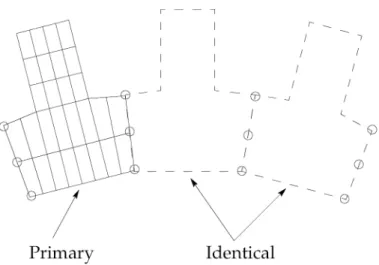
The following figures illustrate the possible types of superelement. Figure 1-1shows a model of a portion of a gear. The physical model of one tooth can be represented as a superelement. This type is called a primary superelement—one where the actual geometry for the superelement is defined in the bulk data.
Other gear teeth, as shown inFigure 1-1, are images of the first (primary) tooth. An image
superelement is one that uses the geometry of another superelement to describe it for NX Nastran. These image superelements can save processing time in that they are able to use the stiffness, mass, and damping from their primary superelement, which reduces the amount of calculations needed. Full data recovery is available for image superelements. An image superelement can be an identical image, as shown inFigure 1-1, or a mirror image, as shown inFigure 1-2. InFigure 1-2, the right side of the plate is a mirror-image copy of the primary. Please note that images can have their own unique loadings. Only the stiffness, mass, and damping are identical to the primary.
Another type of superelement is the external superelement, where a part of the model is represented using matrices from an outside source. (The matrices can come from another NX Nastran run.) For these matrices, no internal geometry information is available; only the grid points to which the matrices are attached are known. An external superelement is shown inFigure 1-3. In this figure the finite element model is on the left and the external superelement is represented by the dashed lines on the right.
Figure 1-1. A Primary and Several Identical Image Superelements.
Figure 1-2. A Primary and a Mirror Image Superelement.
Figure 1-3. An External Superelement.
In static analysis, the theory used in superelement processing is exact. In dynamic analysis, approximations are made in the reduction of the mass, damping, and loading matrices. These approximations are explained in“Introduction to Superelements in Dynamic Analysis”, as are methods (in particular, component modal synthesis) to improve on the approximations.
1.3
Partitioned Solutions
When NX Nastran is processing the bulk data for a model, the input is partitioned into a separate set for each superelement, based on user instructions. The input used to accomplish this partitioning is discussed in“How to Define a Superelement”.
Once the bulk data is partitioned into separate sets, each superelement is processed individually. The degrees-of-freedom (DOFs) for each superelement are partitioned into sets in a manner identical to that used in conventional analysis. That is, all DOFs for a superelement are combined to create a G-set. Then MPCs and R-elements are used to define the M- and N-sets, and so on. (SeeNX Nastran User’s Guidefor a complete description of sets.) The only change in the definition of sets is the definition of exterior DOFs. For each superelement, the exterior DOFs are defined as the A-set. The exterior DOFs are best described as those that are retained for further analysis, or you can think of them as attachment DOFs, where the superelement connects to the rest of the structure. Structural matrices are assembled for each superelement, and the matrices go through reduction processing until the only remaining terms are for the A-set or attachment DOFs. These reduced matrices are used to represent the properties of the superelement when it is attached to the rest of the model. Interior DOFs can be thought of as those that are condensed out during superelement processing. All DOFs of a superelement that are not exterior are called interior DOFs (the omitted or O-set). These DOFs are condensed out of the matrices during the reduction process. Using either a static or dynamic reduction, the stiffness, mass, damping, and loading on these interior DOFs are transferred to the exterior DOFs.
The reduction process is best illustrated using the process known as static condensation. In this process, we start with the superelement matrices after all MPCs, R-elements, and SPCs have been processed. The set of DOFs remaining at this point are in terms of the F-set (DOFs that are not constrained), which contains the O- and A-sets as subsets. Although the interior DOFs include the M-and S-sets also, the interior DOFs in this guide are often referred to as the O-set.
Note
Each superelement is processed individually. The static equation for the F-set is
Equation 1-1.
This equation may be rewritten as
where the bar over a term (for example ) indicates that the sub-matrix represents the associated matrix of terms for that set before the reduction operation. If we look at the upper part of the equation, we obtain
Equation 1-3.
Pre-multiplying both sides of the equation by [Koo]−1gives
Equation 1-4.
At this point we will define some terms:
The static boundary transformation matrix between the exterior and interior motion is calledGot
and is defined as
Equation 1-5. Note
The ‘T’-set is a subset of the ‘A’-set. The ‘T’-set contains any “physical” exterior DOFs. In static analysis, the ‘T’-set is normally identical to the ‘A’-set. In this part of the book—when discussing static analysis—the two will often be used interchangeably.
Physically, this matrix represents the solution to the boundary motion problem. That is, each column of this matrix represents the motion of the interior points when one boundary DOF is moved one unit while the other boundary points are held constrained.
Therefore, the transformation matrix has one column for each exterior (boundary) DOF (the A-set for the superelement), and the number of rows are equal to the number of interior DOFs (the O-set for the superelement).
Also, the fixed-boundary displacements of the superelement are defined as follows:
Equation 1-6.
This matrix represents the static solution for the displacements of the superelement when the loads are applied and the exterior points are held fixed. Based on these definitions, the total displacement of the interior points can be defined as
Equation 1-7.
whereUtis the solution for the displacements of the exterior (boundary) points. We now substitute the equation forUoin the lower part ofEq. 1-2, obtaining
Equation 1-8.
From this expression we obtain the reduced stiffness and loading matrices for the superelement. The reduced stiffness, Kttis defined as
Equation 1-9.
and the reduced loadingPtis defined as
Equation 1-10.
The residual structure consists of all components of the model that were not assigned to any other superelement, plus the assembly of the reduced superelement matrices.
Each superelement is processed in this manner, and its associated matrices are reduced to the exterior DOFs. Once all superelements have been processed, the reduced matrices are assembled into a system matrix during the residual structure processing. The residual structure consists of all components of the model that were not assigned to a superelement, plus the assembly of the reduced superelement matrices.
The system or assembly solution is performed using the assembled matrices for the residual structure. Once the assembly solution is known, the boundary solution is found for each superelement. This boundary solution is used to calculate the interior displacements for each superelement, then standard data recovery is available for all superelements, including the residual structure. Any output that is available in standard (non-superelement) analysis is available in superelement analysis. The difference is that the output is now partitioned by superelement.
1.4
Example to Show the Use of Superelements in Static Analysis
The following small problem demonstrates how a static analysis is performed using superelements. The solution to the problem is first shown using conventional analysis, then using superelements.Figure 1-4.
For this example, we are looking only at motion along the axis of the points, thus the problem is simplified to contain only five DOFs.
Conventional Analysis
In conventional analysis, the problem is formulated in matrix form, constraints are applied, and the resulting reduced problem is solved. The five-by-five stiffness matrix is as follows:
Equation 1-11.
Each row (or column) in the above matrix represents the terms associated with one DOF in the model. The terms are in ascending order, that is, the first column represents DOF 1, and the last column represents DOF 5. Replacing the springs by their numeric values, we have
Equation 1-12.
We now apply the constraints to the problem. In finite element analysis, constraints are applied by removing the associated rows and columns from the matrix; therefore, after applying constraints, we have the static equation for the constrained structure
Equation 1-13.
or, in numeric terms
Equation 1-14.
Solving this equation gives the solution
Superelement Analysis
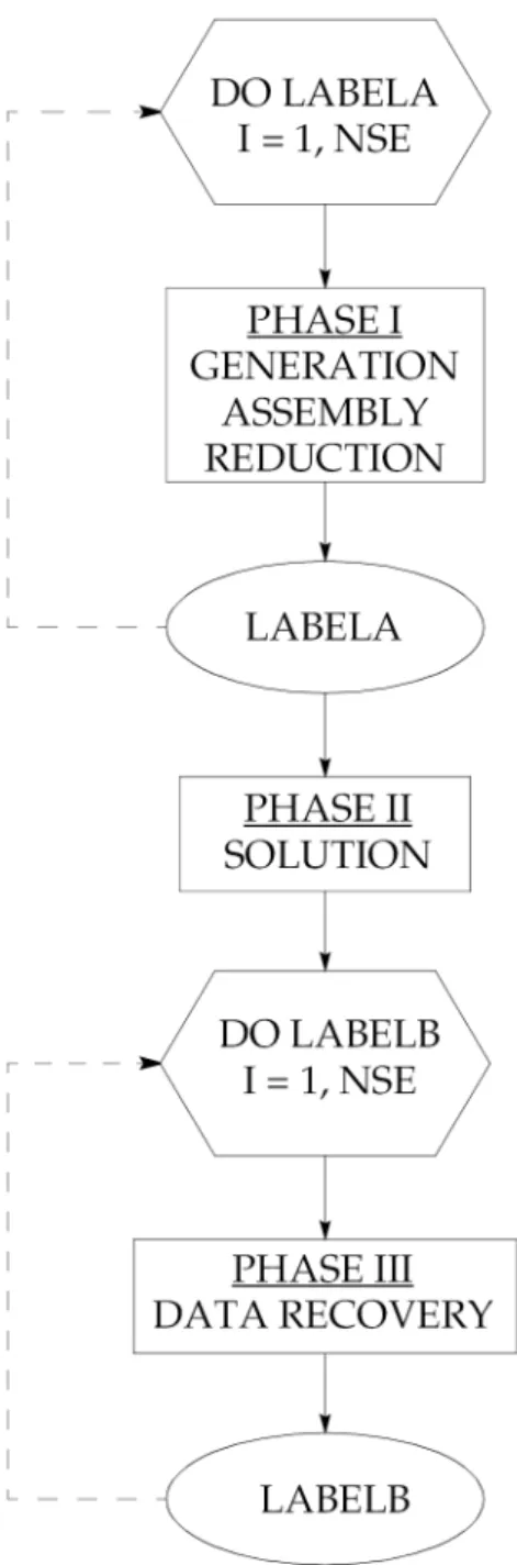
We now formulate and solve the same problem using superelements, as shown inFigure 1-6. Because the method of defining superelements has not been discussed yet, some of what follows has not been defined. However, as you read further, more of the information will become clear. First a flowchart showing the order of processing used to perform superelement analysis is shown in
Figure 1-5.
These three phases (I, II, and III) are used in all superelement solutions and will be referred to later in this guide.
Figure 1-6.
The definitions of the model, as shown previously inFigure 1-6, are as follows: • Superelement 1 (SEID = 1)
Grid points 1 and 2 are interior points. (These grid points are condensed out during the phase one operations for superelement 1.)
ElementsK12andK23are interior or belong to superelement 1. The constraint at grid point 1 is contained in superelement 1. The load applied on grid point 2 is in superelement 1.
Grid point 3 is exterior to superelement 1. (After reduction [Phase 1] is completed for superelement 1, all that remains is a set of matrices representing the superelement attached to grid point 3.)
• Superelement 2 (SEID = 2)
Grid points 4 and 5 are interior to superelement 2. Grid point 3 is exterior to superelement 2.
The load on grid point 4 is in superelement 2.
ElementsK34andK35are interior to or belong to superelement 2. The constraint on grid point 5 is contained in superelement 2. • Residual structure (R.S. OR SEID = 0)
Grid point 3 is interior to the residual structure.
There are no elements left to belong to the residual structure. The load on grid point 3 is in the residual structure.
Superelements 1 and 2 are processed independently, then the reduced matrices are assembled at the residual.
Superelement 1
After the model is divided into superelements, the data for superelement 1 contains the following information:
Figure 1-7.
Based on this model,u3is the exterior DOF and belongs to the A-set for superelement 1. Therefore, we want to generate matrices for superelement 1, apply any constraints, and reduce the matrices to the exterior DOF. The G-set for this superelement consists of the DOFs associated with grid points 1, 2, and 3. The following are the G-sized matrices:
Equation 1-16.
Equation 1-17.
The superscript 1 shown on the matrices indicates that they belong to superelement 1. Notice that the force on grid point 3 (P3) is not included. Because the force is applied to an exterior point, it is not included in the superelement. This fact is indicated in the matrix for the loading by placing a bar over theP3term and indicating that this represents only loading on grid point 3 associated with superelement 1.
Looking at the model, we see that grid point 1 is constrained. Because that grid point is interior to the superelement, the constraint is applied as a part of the processing for superelement 1. The resulting (reduced) stiffness matrix is
Equation 1-18.
This matrix is now divided into interior (O-set) and exterior (A-set) DOFs, and a static condensation is performed to reduce the matrices to the exterior DOFs.
First we compute the boundary transformation:
Equation 1-19.
This transformation states that if point 3 is moved 1.0 units, then point 2 will move .5 units, which is the expected result when point 1 is constrained.
Now the transformation is used to reduce the stiffness matrix to the boundary.
Equation 1-20.
The results make sense. Superelement 1 contains two springs in series, and the resulting stiffness as seen at grid point 3 is 0.5.
Now we have to reduce the applied loadings to the boundary. After applying the constraint to the loading matrix, we have
Equation 1-21.
which can be reduced to the boundary as follows:
Equation 1-22.
Once again, the result is what we would expect. If grid point 3 is constrained and the unit force is applied to grid point 2, the reaction seen at point 3 is 0.5 units.
Superelement 2
The data for superelement 2 contains the following information
Figure 1-8.
u3is the exterior DOF and belongs to the A-set for superelement 2. Therefore, we want to generate matrices for superelement 2, apply any constraints, and reduce the matrices to the exterior DOF.
Equation 1-23.
Equation 1-24.
Notice that the force on grid point 3 does not show up in superelement 2 either. Once again, forces on exterior points are not included in the superelement matrices.
The constraint will be applied, this time at DOF5, then the boundary transformation will be calculated and applied, resulting in the following:
Equation 1-25.
The transformation and reduced matrices make sense. If grid point 3 is moved 1.0 unit, grid point 4 will move 0.5 units. As before, the stiffness is two springs in series, resulting in a combined stiffness of 0.5, and the load of 3.0 units at grid point 4 gives a 1.5 unit reaction at point 3 if it is constrained.
Residual Structure
The remaining structure, or grid point 3, is defined as the residual structure. Matrices are generated for the residual structure, based on any elements or loads remaining, then the reduced matrices from the
superelements are added at the appropriate DOFs. Once the combined assembly matrices exist, any constraints applicable to the remaining DOFs are applied and the residual structure problem is solved.
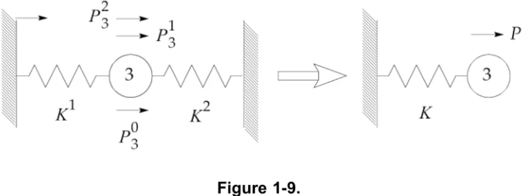
Figure 1-9shows the residual structure. The individual components that are assembled to make up the residual are shown on the left. The resulting assembly model is shown on the right.
The residual structure for this model contains no elements, only one grid point, the physical load on that point, and the reduced matrices from the superelements.
Figure 1-9.
Because all physical constraints have been applied at the superelement level, no reduction is performed at the residual level for this model. If there were a physical model for the residual, then it would also go through the application of constraints and a reduction to a final set of analysis matrices. Therefore, the assembly matrix is the result of adding the superelement matrices together at grid point 3, or
Equation 1-26.
where the matricesK1
aaandK2aarepresent the reduced superelement stiffness matrices, and the
matrixK0
ggrepresents the stiffness matrix resulting from any elements in the residual structure. In
this problem there are no elements in the residual structure; therefore,K0
ggis null.
Similarly, the loading matrix is the physical loadings applied on the residual, plus the reduced superelement loads. The 2 unit force on grid point 3 is finally included at this point, because it is acting on a grid point that is interior to the residual structure.
Equation 1-28.
Now that the stiffness and loading matrices have been generated and reduced, we are ready to solve the residual structure problem for the A-set displacements:
Equation 1-29.
Equation 1-30.
We now have the displacement solution for the residual structure, and we are ready to begin data recovery. Data recovery is processed for each superelement independently, allowing segmented or selective data recovery.
Superelement 1
We already have the solution for the exterior point (grid point 3), and now we are ready to perform data recovery for the interior points of superelement 1. First, we calculate the fixed-boundary solution. That is, we calculate the motion of superelement 1 if the exterior point is held constrained and the loadings are applied.
Figure 1-10.
Figure 1-11.
Finally, by superposition the interior displacement is
Equation 1-31.
which is identical to the solution obtained for grid point 2 when the model was solved without using superelements. Element output, SPC forces, and all other standard output can now be calculated for superelement 1.
Superelement 2
Once again, the boundary solution is known from the residual structure solution, and data recovery is similar to that performed on superelement 1. Data recovery is not shown for superelement 2 but also gives answers identical to the solution obtained without superelements.
Simply stated, a static superelement solution is the combination of the solution obtained by adding the fixed-boundary solution to the solution obtained by imposing the boundary displacements. In static analysis, there are no approximations made using superelements.
Sample Problem
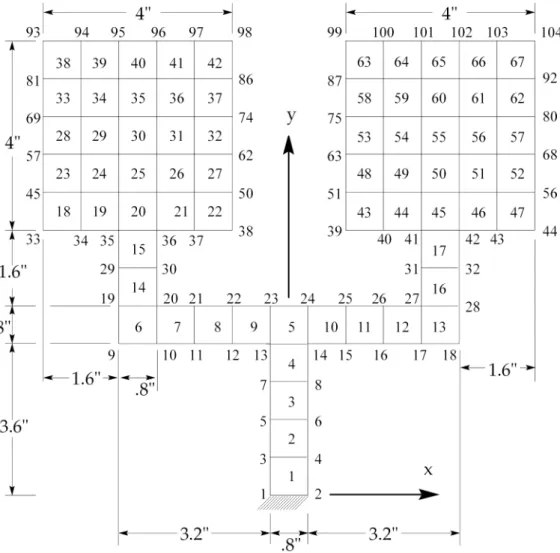
For consistency, throughout this guide the model shown inFigure 1-12is used as a sample problem to demonstrate NX Nastran input and output. The model, best described as a metal stamping (also known as a two-headed flyswatter), has absolutely no resemblance to any real problem. The reasons for this choice are as follows: Most real models are much too complicated to be used as a simple example (the input is too cumbersome), and a model that might be reasonable to people working in one industry may have no meaning whatsoever to someone in another industry. The model is simple and needs no description.
The bulk data for the model is shown inListing 1-1. This listing uses replicators to generate many of the entries and is not shown again in this guide. In subsequent chapters and examples, this listing is
referred to using the INCLUDE entry. In this way, listings shown in this guide contain only information specific for that run, resulting in less confusion.
Figure 1-12. Two-Headed Flyswatter.
The structure is made of steel with Young’s modulus of 30,000,000 psi, weight density of 0.283 lb/in.3, and Poisson’s ratio of 0.3. Grid points 1 and 2 are constrained. In static analysis, the structure will undergo three loadings:
• Pressure applied on elements 18 through 67.
• Point loads of two pounds acting in the positive Z direction at grid points 93 and 104. • Opposing two pound point loads in the Z direction at grid points 93 and 104.
Table 1-1. Listing of Bulk Data for the Sample Problem.
$
$ ************************************************************** $ BASIC MODEL DEFINITION - SAME FOR ALL RUNS
$ ************************************************************** $
$ FILE NAME IS MODEL.DAT $ GRDSET,,,,,,,6 GRID,1,,-.4,0.,0.,,123456 GRID,3,,-.4,0.9,0. =,*2,=,=,*.9,== =1 GRID,2,,.4,0.,0.,,123456 GRID,4,,.4,0.9,0. =,*2,=,=,*.9,== =1 GRID,9,,-3.6,3.6,0. =,*1,=,*.8,== =8 GRID,19,,-3.6,4.4,0. =,*1,=,*.8,== =8 GRID,29,,-3.6,5.2,0. GRID,30,,-2.8,5.2,0. GRID,31,,2.8,5.2,0. GRID,32,,3.6,5.2,0. GRID,33,,-5.2,6.,0. =,*1,=,*.8,== =4 GRID,39,,1.2,6.,0. =,*1,=,*.8,== =4 GRID,45,,-5.2,6.8,0. =,*1,=,*.8,== =4 GRID,51,,1.2,6.8,0. =,*1,=,*.8,== =4 GRID,57,,-5.2,7.6,0. =,*1,=,*.8,== =4 GRID,63,,1.2,7.6,0. =,*1,=,*.8,== =4 GRID,69,,-5.2,8.4,0. =,*1,=,*.8,== =4 GRID,75,,1.2,8.4,0. =,*1,=,*.8,== =4 GRID,81,,-5.2,9.2,0. =,*1,=,*.8,== =4 GRID,87,,1.2,9.2,0. =,*1,=,*.8,== =4 GRID,93,,-5.2,10.,0. =,*1,=,*.8,== =4 GRID,99,,1.2,10.,0. =,*1,=,*.8,== =4 $ $ ELEMENTS
Table 1-1. Listing of Bulk Data for the Sample Problem. $ CQUAD4,1,1,1,2,4,3 =,*1,=,*2,*2,*2,*2 =1 CQUAD4,4,1,7,8,14,13 CQUAD4,6,1,9,10,20,19 =,*1,=,*1,*1,*1,*1 =2 CQUAD4,5,1,13,14,24,23 CQUAD4,10,1,14,15,25,24 =,*1,=,*1,*1,*1,*1 =2 CQUAD4,14,1,19,20,30,29 CQUAD4,15,1,29,30,36,35 CQUAD4,16,1,27,28,32,31 CQUAD4,17,1,31,32,42,41 CQUAD4,18,1,33,34,46,45 =,*1,=,*1,*1,*1,*1 =3 CQUAD4,23,1,45,46,58,57 =,*1,=,*1,*1,*1,*1 =3 CQUAD4,28,1,57,58,70,69 =,*1,=,*1,*1,*1,*1 =3 CQUAD4,33,1,69,70,82,81 =,*1,=,*1,*1,*1,*1 =3 CQUAD4,38,1,81,82,94,93 =,*1,=,*1,*1,*1,*1 =3 CQUAD4,43,1,39,40,52,51 =,*1,=,*1,*1,*1,*1 =3 CQUAD4,48,1,51,52,64,63 =,*1,=,*1,*1,*1,*1 =3 CQUAD4,53,1,63,64,76,75 =,*1,=,*1,*1,*1,*1 =3 CQUAD4,58,1,75,76,88,87 =,*1,=,*1,*1,*1,*1 =3 CQUAD4,63,1,87,88,100,99 =,*1,=,*1,*1,*1,*1 =3 MAT1,1,30.+6,,.3,.283 PARAM,WTMASS,.00259 PARAM,AUTOSPC,YES PSHELL,1,1,.05,1,,1 $ $ ******************************************************************* $ END OF BASIC MODEL DEFINITION
• Defining a Superelement Using Partitioned Bulk Data (PARTs)
• Defining Superelements in the Main Bulk Data Section
Now that the basic concept of superelements has been explained, it is time to learn how to define superelements in NX Nastran. Superelements are defined using the Bulk Data Section of the input file. There are two methods available for defining superelements: main bulk data superelements and PARTs.
The following sections provide a description of each method, with examples. Each superelement in NX Nastran is identified by an integer identification known as the SEID. Each SEID must be a unique positive integer (with the exception of the residual structure, which is known as superelement 0). If no superelements are defined, the model is assumed to be a residual-structure-only model, and a conventional (non-superelement) solution is performed. By default, all superelement solutions perform a conventional solution if no superelements are defined.
As the name implies, main bulk data superelements are defined in the Main Bulk Data Section of the input file. When superelements are defined using this approach, the model defined in this section of the input is divided into separate components. (Each component is a superelement.) A good way to describe this is to say that the program is using a cookie-cutter approach with the model, taking a complete model and dividing it into superelements.
PART superelements are defined in a different manner. Each superelement is defined in its own Partitioned Bulk Data Section. These separate sections of the bulk data are self-contained in that each section contains all geometry, elements, properties, constraints, and loading data for that component of the model. When PARTs are used, the program works in a manner similar to an assembly process. That is, a series of separate components are assembled into the final finite element model.
An external superelement is a reduced boundary representation of a full component model stored in an external file such as an .op2, .op4, bulk data, or database. After you create several external superelements in specific “creation” solutions, you can then combine them in a full NX Nastran system analysis.
All of these approaches can be used independently or together.
2.1
Defining a Superelement Using Partitioned Bulk Data
Defining PARTs
PARTs are defined as separate components using separate areas of the Bulk Data Section.
Therefore, each PART can be thought of as a separate component model. NX Nastran automatically locates any coincident grid points in the PARTs and connects the component models to create the assembly model.
The Bulk Data Section can be divided into separate sections for each PART. This division is accomplished by using the BEGIN SUPER entry. The format of this entry is as follows:
whereiis the superelement id being defined. The commonly used form of this command is:
Prior to MSC.Nastran Version 69, the Bulk Data Section of the input file was a single section of data with the exception of auxmodels in optimization, which contained the complete model definition. The entire model was defined in the area between BEGIN BULK and ENDDATA. Each grid point had to be unique, and each element ID had to be unique. In MSC.Nastran Version 69, it became possible to partition the Bulk Data Section of the input into separate component models, using the BEGIN SUPER command. Thus, each of these component models is a self-contained model defining a PART of the total model. Within each of these sections, grid point and element IDs must be unique as before; however, different PARTs can reuse grid and element IDs, because the sections are separate in the input file.
The Bulk Data Section Using PARTs
When PARTs are used, the bulk data is divided into different sections. The section of the bulk data contained between the BEGIN BULK and either the first BEGIN SUPER or the ENDDATA is known as the Main Bulk Data Section. If only this area is used, then the file is compatible with versions of MSC.Nastran prior to Version 69. In this section, superelements can be defined (although it is not required) using the method shown in“Defining Superelements in the Main Bulk Data Section.”Any superelements defined in this section are known as main bulk data superelements.
When you define PARTs, it is not necessary for you to tell NX Nastran where to make the connections to other superelements. The program contains logic to determine which grid points are coincident and automatically connects (by default) any coincident grid points. Later in this section, we discuss how to override the automatic connection.
Format of the Input File When PARTs Are Used
When PARTs are used, the Executive and Case Control Sections are unchanged; only the Bulk Data Section is different. A sample input file looks like the following:
SOL 101 CEND
TITLE = Sample Input File Demonstrating PARTs .
.
BEGIN BULK $
$ MAIN BULK DATA SECTION $
. .
BEGIN SUPER = 1 $
$ data for PART 1 $
. .
BEGIN SUPER = 25 $
$ data for PART 25 $
. . ENDDATA
In this example, there is a Main Bulk Data Section (in which you can define some main bulk data superelements) and two PART superelements (1 and 25). Each section is self-contained. That is, no entry in PART 1 can reference an entry in any other section of the input. This goes for all PARTs; they
must be self-contained. There are several main bulk data entries that can be used to move, copy, or manually connect PARTs, but beyond these entries, no entry in any section of the input can reference an entry in any other section of the bulk data.
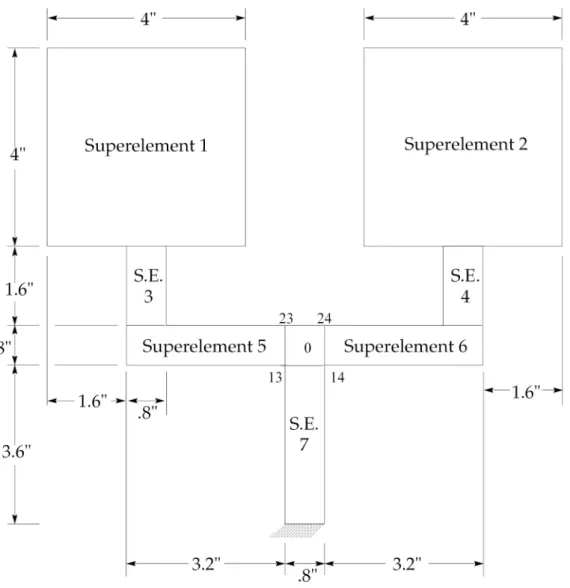
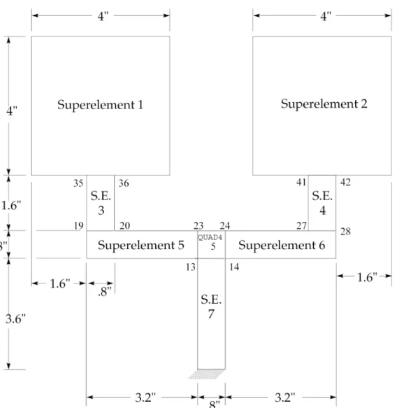
We will look at how to define the two-headed flyswatter model (from the previous section) using PARTs. We are going to define the model using seven PART superelements and a residual structure. The figure below shows how the model will be divided into superelements.
Figure 2-1. Residual Structure for the Sample Problem Divided into Superelements.
Each superelement in this model is defined using a PART or a separate section of the bulk data. Therefore, there are seven separate BEGIN SUPER sections in our input file. The residual structure is defined in the main bulk data. (This is not required; we are simply showing that this is an option.) The following input file is used to solve this problem:
$
$ file - se1s101p.dat $
$ all 7 s.e. brought in using begin super $ duplicate boundary grid ids
$ SOL 101 CEND
TITLE = S.E. SAMPLE PROBLEM 1
SUBTITLE = S.E. STATICS - RUN 1 - MULTIPLE LOADS DISP = ALL
$
$ default is super = all for V69 $
$ set defaults for all se - see section 5 $
PARAM,GRDPNT,0 PARAM,WTMASS,.00259 SUBCASE 101
LABEL = PRESSURE LOAD LOAD = 101
$
SUBCASE 201
LABEL = 2# NORMAL LOADS LOAD = 201
$
SUBCASE 301
LABEL = OPPOSING LOADS LOAD = 301 $ include ’plot.dat’ $ BEGIN BULK $
$ main bulk data section $ include ’part0.dat’ $ begin super=1 $ include ’loadprt1.dat’ include ’part1.dat’ $ begin super=2 $ include ’loadprt2.dat’ include ’part2.dat’ $ begin super=3 $ include ’part3.dat’ $ begin super=4 $ include ’part4.dat’ $ begin super=5 $ include ’part5.dat’ $ begin super=6 $ include ’part6.dat’ $ begin super=7 $ include ’part7.dat’ $ enddata
The listings of the included files are given below. The executive control selects SOL 101, which is the static solution that includes superelements. The case control defines three solutions for this model and provides default parameter values for all superelements in the model (a detailed description of the case control for superelements is in Section 5). The file plot.dat is a file requesting plots and is not shown until the section describing superelement plotting.
The Main Bulk Data Section of the file is very short; for this model it contains the physical model of the residual structure. This model is defined in the file part0.dat, which is shown here:
CQUAD4 5 1 13 14 24 23 $ GRDSET 6 GRID 13 -.4 3.6 0. GRID 14 .4 3.6 0. GRID 23 -.4 4.4 0. GRID 24 .4 4.4 0. $ MAT1,1,30.+6,,.3,.283 PSHELL,1,1,.05,1,,1 $ param,wtmass,.002588
This file contains the physical model of the residual structure, which consists of element 5 and the grid points to which it is attached, along with the associated properties and parameters. Notice that this file contains only the above information and does not contain copies of the grid points that are used to make the connection between PARTs. (You can place copies of these points in the residual structure if you wish—the answers are the same for single-level solutions). The model of the residual structure ends with the end of the Main Bulk Data Section or at the BEGIN SUPER = 1. Subsequent entries belong to the PARTs.
The section of the input file defining PART 1 is next and contains two include statements. These statements insert two files, loadprt1.dat (loading data) and part1.dat (the model of the PART), into the runstream. These two files follow.
$
$ file - loadprt1.dat $ loads on s.e. 1 $
$ LOAD CASE 1 - PRESSURE LOAD $
PLOAD2,101,-1.,18,THRU,42 $
$ LOAD CASE 2 - 2 POINT LOADS AT CORNERS $
FORCE,201,93,,2.,0.,0.,1. $
$ LOAD CASE 3 - OPPOSING POINT LOADS AT CORNERS $
FORCE,301,93,,2.,0.,0.,1. $
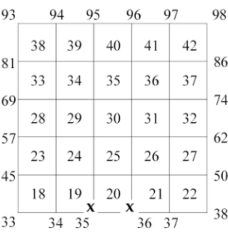
File loadprt1.dat contains the data that defines the loadings to be applied to PART 1 for the three static solutions. $ $ part1.dat $ CQUAD4 18 1 33 34 46 45 CQUAD4 19 1 34 35 47 46 CQUAD4 20 1 35 36 48 47 CQUAD4 21 1 36 37 49 48 CQUAD4 22 1 37 38 50 49 CQUAD4 23 1 45 46 58 57
CQUAD4 24 1 46 47 59 58 CQUAD4 25 1 47 48 60 59 CQUAD4 26 1 48 49 61 60 CQUAD4 27 1 49 50 62 61 CQUAD4 28 1 57 58 70 69 CQUAD4 29 1 58 59 71 70 CQUAD4 30 1 59 60 72 71 CQUAD4 31 1 60 61 73 72 CQUAD4 32 1 61 62 74 73 CQUAD4 33 1 69 70 82 81 CQUAD4 34 1 70 71 83 82 CQUAD4 35 1 71 72 84 83 CQUAD4 36 1 72 73 85 84 CQUAD4 37 1 73 74 86 85 CQUAD4 38 1 81 82 94 93 CQUAD4 39 1 82 83 95 94 CQUAD4 40 1 83 84 96 95 CQUAD4 41 1 84 85 97 96 CQUAD4 42 1 85 86 98 97 $ GRDSET 6 $ $ boundary grids $ GRID 35 -3.6 6. 0. GRID 36 -2.8 6. 0. $ GRID 33 -5.2 6. 0. GRID 34 -4.4 6. 0. GRID 37 -2. 6. 0. GRID 38 -1.2 6. 0. $ GRID 45 -5.2 6.8 0. GRID 46 -4.4 6.8 0. GRID 47 -3.6 6.8 0. GRID 48 -2.8 6.8 0. GRID 49 -2. 6.8 0. GRID 50 -1.2 6.8 0. GRID 57 -5.2 7.6 0. GRID 58 -4.4 7.6 0. GRID 59 -3.6 7.6 0. GRID 60 -2.8 7.6 0. GRID 61 -2. 7.6 0. GRID 62 -1.2 7.6 0. GRID 69 -5.2 8.4 0. GRID 70 -4.4 8.4 0. GRID 71 -3.6 8.4 0. GRID 72 -2.8 8.4 0. GRID 73 -2. 8.4 0. GRID 74 -1.2 8.4 0. GRID 81 -5.2 9.2 0. GRID 82 -4.4 9.2 0. GRID 83 -3.6 9.2 0. GRID 84 -2.8 9.2 0. GRID 85 -2. 9.2 0. GRID 86 -1.2 9.2 0. GRID 93 -5.2 10. 0. GRID 94 -4.4 10. 0. GRID 95 -3.6 10. 0. GRID 96 -2.8 10. 0. GRID 97 -2. 10. 0. GRID 98 -1.2 10. 0. $ MAT1,1,30.+6,,.3,.283 PARAM,WTMASS,.00259 PARAM,AUTOSPC,YES
PSHELL,1,1,.05,1,,1 $
File part1.dat contains the physical model for PART1. If you look at the illustration of the model provided in the previous section, you will notice that this PART attaches to PART 3 at grid points 35 and 36. Notice that these points are contained in the data for this component of the model.
PART 2 is defined by similar files (shown later in this section) and will not be discussed here. PART 3 is defined by a single file, part3.dat:
$ $ part3.dat $ CQUAD4 14 1 19 20 30 29 CQUAD4 15 1 29 30 36 35 $ GRDSET 6 $ $ boundary grids $ GRID 19 -3.6 4.4 0. GRID 20 -2.8 4.4 0. GRID 35 -3.6 6. 0. GRID 36 -2.8 6. 0. $ GRID 29 -3.6 5.2 0. GRID 30 -2.8 5.2 0. $ MAT1,1,30.+6,,.3,.283 PARAM,WTMASS,.00259 PARAM,AUTOSPC,YES PSHELL,1,1,.05,1,,1 $
This file contains the physical model for PART 3. This PART connects to PART 1 at grid points 35 and 36 (both included in this section) and also connects to PART 5 at grid points 19 and 20 (also included in this section). When processing PARTs, NX Nastran looks for grid points that are coincident, such as grid points 35 and 36 in PART 1 and grid points 35 and 36 in PART 3. Unless instructed otherwise, the program connects these components at these points. Therefore, grid points 35 and 36 are exterior to superelement 1. There is no requirement that the grid points have the same ID in different PARTs, only that they be coincident within a tolerance (described later). When coincident points are found, the program notes that they should be connected and (unless there is a coincident point in the residual structure model or you are using a multi-level tree) creates an internal grid point in the residual structure model that is coincident with these points. The matrices for each component are reduced to the external DOFs and passed downstream to the residual structure, where the matrices are combined and solved.
All boundary grids are identified in the output from NX Nastran (see output from this sample in Section 9) and listed as exterior (or interior) to the appropriate superelements. Once all PARTs have been read and all coincident grid points have been found, the program is ready to process the PARTs. The following files are the rest of the input for this example.
$ $ part2.dat $ CQUAD4 43 1 39 40 52 51 CQUAD4 44 1 40 41 53 52 CQUAD4 45 1 41 42 54 53 CQUAD4 46 1 42 43 55 54 CQUAD4 47 1 43 44 56 55
CQUAD4 48 1 51 52 64 63 CQUAD4 49 1 52 53 65 64 CQUAD4 50 1 53 54 66 65 CQUAD4 51 1 54 55 67 66 CQUAD4 52 1 55 56 68 67 CQUAD4 53 1 63 64 76 75 CQUAD4 54 1 64 65 77 76 CQUAD4 55 1 65 66 78 77 CQUAD4 56 1 66 67 79 78 CQUAD4 57 1 67 68 80 79 CQUAD4 58 1 75 76 88 87 CQUAD4 59 1 76 77 89 88 CQUAD4 60 1 77 78 90 89 CQUAD4 61 1 78 79 91 90 CQUAD4 62 1 79 80 92 91 CQUAD4 63 1 87 88 100 99 CQUAD4 64 1 88 89 101 100 CQUAD4 65 1 89 90 102 101 CQUAD4 66 1 90 91 103 102 CQUAD4 67 1 91 92 104 103 $ GRDSET 6 $ $ boundary grids $ GRID 41 2.8 6. 0. GRID 42 3.6 6. 0. $ GRID 39 1.2 6. 0. GRID 40 2. 6. 0. GRID 43 4.4 6. 0. GRID 44 5.2 6. 0. $ GRID 51 1.2 6.8 0. GRID 52 2. 6.8 0. GRID 53 2.8 6.8 0. GRID 54 3.6 6.8 0. GRID 55 4.4 6.8 0. GRID 56 5.2 6.8 0. GRID 63 1.2 7.6 0. GRID 64 2. 7.6 0. GRID 65 2.8 7.6 0. GRID 66 3.6 7.6 0. GRID 67 4.4 7.6 0. GRID 68 5.2 7.6 0. GRID 75 1.2 8.4 0. GRID 76 2. 8.4 0. GRID 77 2.8 8.4 0. GRID 78 3.6 8.4 0. GRID 79 4.4 8.4 0. GRID 80 5.2 8.4 0. GRID 87 1.2 9.2 0. GRID 88 2. 9.2 0. GRID 89 2.8 9.2 0. GRID 90 3.6 9.2 0. GRID 91 4.4 9.2 0. GRID 92 5.2 9.2 0. GRID 99 1.2 10. 0. GRID 100 2. 10. 0. GRID 101 2.8 10. 0. GRID 102 3.6 10. 0. GRID 103 4.4 10. 0. GRID 104 5.2 10. 0. $ MAT1,1,30.+6,,.3,.283 PARAM,WTMASS,.00259
PARAM,AUTOSPC,YES PSHELL,1,1,.05,1,,1 $ $ $ file - loadprt2.dat $ loads on s.e. 2 $
$ LOAD CASE 1 - PRESSURE LOAD $
PLOAD2,101,-1.,43,THRU,67 $
$ LOAD CASE 2 - 2 POINT LOADS AT CORNERS $
FORCE,201,104,,2.,0.,0.,1. $
$ LOAD CASE 3 - OPPOSING POINT LOADS AT CORNERS $ FORCE,301,104,,2.,0.,0.,-1. $ $ $ part4.dat $ CQUAD4 16 1 27 28 32 31 CQUAD4 17 1 31 32 42 41 $ GRDSET 6 $ $ boundary grids $ GRID 27 2.8 4.4 0. GRID 28 3.6 4.4 0. GRID 41 2.8 6. 0. GRID 42 3.6 6. 0. $ GRID 31 2.8 5.2 0. GRID 32 3.6 5.2 0. $ MAT1,1,30.+6,,.3,.283 PARAM,WTMASS,.00259 PARAM,AUTOSPC,YES PSHELL,1,1,.05,1,,1 $ $ $ part5.dat $ CQUAD4 6 1 9 10 20 19 CQUAD4 7 1 10 11 21 20 CQUAD4 8 1 11 12 22 21 CQUAD4 9 1 12 13 23 22 $ GRDSET 6 $ $ boundary grids $ GRID 19 -3.6 4.4 0. GRID 20 -2.8 4.4 0. GRID 13 -.4 3.6 0. GRID 23 -.4 4.4 0. $ GRID 9 -3.6 3.6 0. GRID 10 -2.8 3.6 0. GRID 11 -2. 3.6 0. GRID 12 -1.2 3.6 0. GRID 21 -2. 4.4 0.
GRID 22 -1.2 4.4 0. $ MAT1,1,30.+6,,.3,.283 PARAM,WTMASS,.00259 PARAM,AUTOSPC,YES PSHELL,1,1,.05,1,,1 $ $ $ part6.dat $ CQUAD4 10 1 14 15 25 24 CQUAD4 11 1 15 16 26 25 CQUAD4 12 1 16 17 27 26 CQUAD4 13 1 17 18 28 27 $ GRDSET 6 $ $ boundary grids $ GRID 27 2.8 4.4 0. GRID 28 3.6 4.4 0. GRID 14 .4 3.6 0. GRID 24 .4 4.4 0. $ GRID 15 1.2 3.6 0. GRID 16 2. 3.6 0. GRID 17 2.8 3.6 0. GRID 18 3.6 3.6 0. $ GRID 25 1.2 4.4 0. GRID 26 2. 4.4 0. $ MAT1,1,30.+6,,.3,.283 PARAM,WTMASS,.00259 PARAM,AUTOSPC,YES PSHELL,1,1,.05,1,,1 $ $ $ part7.dat $ CQUAD4 1 1 1 2 4 3 CQUAD4 2 1 3 4 6 5 CQUAD4 3 1 5 6 8 7 CQUAD4 4 1 7 8 14 13 $ GRDSET 6 $ GRID 1 -.4 0. 0. 123456 GRID 2 .4 0. 0. 123456 GRID 3 -.4 0.9 0. GRID 4 .4 0.9 0. GRID 5 -.4 1.8 0. GRID 6 .4 1.8 0. GRID 7 -.4 2.7 0. GRID 8 .4 2.7 0. $ $ boundary grids $ GRID 13 -.4 3.6 0. GRID 14 .4 3.6 0. $ MAT1,1,30.+6,,.3,.283 PARAM,WTMASS,.00259 PARAM,AUTOSPC,YES PSHELL,1,1,.05,1,,1
$
Automatically Connecting PARTs to Other Components of the Model
By default, the program automatically connects points from a PART to any coincident points in any other PARTs or in the Main Bulk Data Section. There is no need to be concerned with coordinate systems on these coincident points; NX Nastran automatically connects coincident points, accounting for differences in the output coordinate systems.
These points are identified as boundary points in the output from NX Nastran. By default, no special effort is required from you to make the connection. If for one connection all the boundary points belong to PARTs (none of the coincident points are in the residual structure), then NX Nastran creates a new point internally that is coincident with the boundary points and places that internal point in the residual structure (or the lowest connected superelement in a multi-level tree). These internal points can not be constrained. If you wish to apply a constraint on this point, you can define a coincident grid point in the residual structure (or in the lowest connected superelement for a multi-level tree) and constrain that point, or you can apply constraints in the PARTs (subject to the limitations in the next paragraph).
Constraints on Connecting Points
If you need to apply constraints on the points where two or more PARTs connect, there are limitations. If you wish to constrain all six DOFs, there is no limitation; place the constraint on the connecting grid point in any of the PARTs and all other coincident points are also constrained in all six DOFs. If the constraint is not on all six DOFs, then you must exercise care. Because the program will allow the connection of coincident points that have different output coordinate systems, it would be difficult to allow constraints on one of the points in one coordinate system and to correctly map that set of constraints onto another system. Therefore, the following set of rules is enforced at connecting points: • If the PARTs being connected are at the same level in the superelement tree, either all six or
none of the DOFs must be constrained.
• If one of the PARTs is at a lower level in the tree, then you must apply the desired constraints at the connection inside the PART that is lowest in the processing tree (last of the group to be processed).
Controlling the Connection Between PARTs and the Rest of the Model
The SEBNDRY, SEBULK, SECONCT, and SEEXCLD entries can appear only in the Main Bulk Data Section of your input file.
If you want to override the automatic connection, there are several options available to you. You can control this operation by using the SEBNDRY, SEBULK, SECONCT, and SEEXCLD entries in the Main Bulk Data Section of your input file.
Although a more thorough explanation follows, here is a quick definition of each of these entries: SEBNDRY Provides a list of grid points that can be connected between a PART and one or
more PARTs (used to limit the automatic search for coincident points).
SECONCT Explicitly defines the GRIDs and SPOINTs to be connected between PARTs (overrides automatic search logic) and allows you to set the tolerance for the coincident point test.
SEEXCLD Provides a list of points in a PART that cannot be connected to one or more other PARTs (used to limit automatic search logic).
The default tolerance in the coincident grid search logic is 1.0E-5 units.
By default, NX Nastran uses the automatic logic to find coincident points between a PART and the other superelements in a model. The default tolerance on the search is 1.0E-5 units. This default can be changed by using either the SEBULK or SECONCT entry.
SEBNDRY
The format of theSEBNDRYentry follows:
Format:
1 2 3 4 5 6 7 8 9 10
SEBNDRY SEIDA SEIDB GIDA1 GIDA2 GIDA3 GIDA4 GIDA5 GIDA6
GIDA7 GIDA8
-etc.-This entry is used to limit the automatic search logic to selected grid points. Any grid points listed on this entry are the only grid points in SEIDA to which the automatic logic can connect grid points in SEIDB.
Description of the fields on this entry:
SEIDA PART for which this entry is used in the automatic search routines.
SEIDB PART(s) for which the search logic uses this list when searching for points coincident to the ones in SEIDA, listed here. This field either contains an integer superelement IDor the wordALL, if the list is used for all superelements when searching for coincident points for SEIDA.
GIDAi Grid points in SEIDA that can be connected to SEIDB if there are coincident points in SEIDB.
Example 1:
1 2 3 4 5 6 7 8 9 10
SEBNDRY 400 4 10 20 30 40
This entry states that when searching for grid points in superelement 4 that are coincident to points in PART 400, only grid points 10, 20, 30, and 40 in PART 400 can be used. No other grid points in superelement 400 can be connected to points in superelement 4, even if they are coincident.
SEBULK
The format of theSEBULKentry is as follows:
Format:
1 2 3 4 5 6 7 8 9 10
SEBULK SEID TYPE RSEID METHOD TOL LOC
This entry has a number of uses. For purposes of the current section, we only discuss using it to control the automatic search logic for coincident grid points.
In this context, a description of the fields on this entry follows:
SEID Superelement number for which this SEBULK entry is being used. You can have SEBULK entries for each PART in your model.
TYPE There are several TYPEs allowed. For purposes of the current discussion, only PRIMARY is considered. (The other TYPEs involve more advanced features.)—no default value.
RSEID Reference superelement ID—also an advanced feature to be discussed later. METHOD Boundary GRID point search method—can beAUTO(default) orMANUAL. If this is
MANUAL, then SECONCT entries must be used for this PART to make the connections to the rest of the model.
TOL Location tolerance for coincident grid point test (default = 1.E-5).
LOC Coincident grid point test option for MANUAL connection. Can beYES(default = grid points must be within TOL, or a FATAL will be issued) orNO. (Do not test for coincidence—may be dangerous).
Example:
1 2 3 4 5 6 7 8 9 10
SEBULK 14 PRIMARY AUTO 1.0E-3
This entry instructs NX Nastran to use the automatic coincident grid point search logic to find the attachment points for superelement 14, but to use a tolerance of 1.0E-3 units.
SECONCT
The format of theSECONCT entry follows:
Format:
1 2 3 4 5 6 7 8 9 10
1 2 3 4 5 6 7 8 9 10
GIDA1 GIDB1 GIDA2 GIDB2 GIDA3 GIDB3
-etc.-This entry manually specifies points (GRID or SPOINT) to be connected between two superelements. If this entry is used and METHOD=AUTO on the SEBULK entry, these points are added to the list of points found by the automatic logic. If METHOD=MANUAL on the SEBULK, only these points are connected between these two superelements.
The fields on this entry are used as follows:
SEIDA PART to be connected.
SEIDB Superelement to which the connection is being made.
TOL Same meaning as on the SEBULK. (Values provided on SECONCT entries override the values provided on the SEBULK.)
LOC Same meaning as on SEBULK. (Values provided on SECONCT entries override the values provided on the SEBULK.)
GIDAi, GIDBi Pairs of grid points to be connected. GIDAi in SEIDA are connected to GIDBi in SEIDB if the coincident tolerance test is satisfied (unless overridden using LOC).
Example:
1 2 3 4 5 6 7 8 9 10
SECONCT 10 20 1.0E-4 YES
1001 4001 1002 4002 2222 4444
This entry states that when connecting PART 10 to superelement 20, the tolerance for the coincident grid point test will be 1.0E-4 units and the coincident point test will be performed. This entry also states that we wish to connect point 1001 in PART 10 to point 4001 in superelement 20, point 1002 in PART 10 to point 4002 in superelement 20, and point 2222 in PART 10 to point 4444 in superelement 20. (In this context, point can apply to sets of either GRID entries or SPOINTs.)
SEEXCLD
The format of the SEEXCLD entry follows:
Format:
1 2 3 4 5 6 7 8 9 10
SEEXCLD SEIDA SEIDB GIDA1 GIDA2 GIDA3 GIDA4 GIDA5 GIDA6
-etc.-This entry is used to limit the automatic search logic. While the SEBNDRY limits the search to selected grid points, the SEEXCLD excludes grid points from the search. Any grid points listed on this entry are grid points in SEIDA that the automatic logic cannot connect to grid points in SEIDB.
Description of the fields on this entry:
SEIDA PART for which this entry is used in the automatic search routines.
SEIDB PART(s) for which the search logic uses this list when searching for points coincident to the ones in SEIDA, listed here. This field contains either an integer superelement ID or the wordALLif the list is used for all superelements, when searching for coincident points for SEIDA.
GIDAi Grid points in SEIDA that cannot be connected to SEIDB if there are coincident points in SEIDB.
Example 2:
1 2 3 4 5 6 7 8 9 10
SEEXCLD 110 10 45 678 396
The above entry states that when connecting PART 110 to superelement 10, grid points 45, 678, and 396 in PART 110 are not considered by the automatic logic.
To show another example of the usage of these entries, we will look at the model used earlier in this section. When we are connecting PART 1 to PART 3, grid points 35 and 36 (which have the same number in both PARTs) are used. This connection can be made in several ways: The example used the automatic connection logic, which determines that these grid points are coincident and connects them; or we could connect these PARTs manually, using the SECONCT entry as follows:
1 2 3 4 5 6 7 8 9 10
SECONCT 1 3
35 35 36 36
This entry would not replace the automatic search logic, rather it would confirm that we want to make this connection, in addition to any found by the search logic. If a SEBULK entry were included with METHOD set to MANUAL, then this entry would replace the automatic search logic.
One way to simplify the internal search is to tell the program that only grid points 35 and 36 in PART 1 can be connected to any other superelement.
1 2 3 4 5 6 7 8 9 10
SEBNDRY 1 ALL 35 36
By doing this, the search logic for connections for PART 1 is simplified. Only grid points 35 and 36 in PART 1 can connect to any other superelement in the model.
Once again, the automatic logic makes the desired connection. The reason for these entries (SEBNDRY, SEBULK, SECONCT, SEEXCLD) is to allow you more control over the search logic. By
default, the automatic logic connects any coincident grid points. Using these entries, you can change from fully automatic to semi-automatic (SECONCT plus automatic or the SEBNDRY or SEEXCLD) or manual (METHOD=MANUAL on the SEBULK with a SECONCT). The choice is yours. The logic for the automatic connection is very efficient. In our testing, it took only a few seconds to search over 1,000,000 grid points to find all coincident points in a model. Compared to the amount of time to be spent solving this problem, this amount of time is negligible.
Manually Defining Exterior Points for a PART
When defining a PART it is possible to use ASET, BSET, CSET and/or ASET1, BSET1, CSET1 entries to define exterior points. Any point in a PART that is listed on either an ASET or ASET1 entry is automatically made exterior to that PART (whether there is a coincident point in another superelement or not). All six DOFs of that point are made exterior. The fields on these entries that are used to select DOFs are ignored when these entries are used in PARTs. If there is no coincident point in any other PART, internal points are created in the residual structure that are coincident with the selected points, and the matrices for the PART are connected to these points.
Moving and/or Rotating PARTs
If the model of a PART is not in the correct location or orientation, you can move and/or rotate the part with NX Nastran before the program tries to connect it to the other components of the model. This moving and rotating is accomplished using the SELOC entry in the Main Bulk Data Section.
Format:
1 2 3 4 5 6 7 8 9 10
SELOC SEID PA1 PA2 PA3 PB1 PB2 PB3
This entry instructs NX Nastran to move and/or rotate a PART using three non-collinear GRID entries in the PART and three GRID entries or POINTs (defined in the Main Bulk Data Section), which are located where you would like those entries (in the PART) to be.
The fields on this entry are described as follows:
SEID PART that is being translated and/or rotated.
PA1-PA3 Three GRID entries in the PART that are to be used to move the PART. After moving, these points will be coincident with PB1-PB3.
PB1-PB3 Three points (either GRID or POINT entries) defined in the Main Bulk Data Section that define where the PART should be.
When this entry is encountered, the program relocates the PART so that grid points PA1-PA3 in the PART are coincident with PB1-PB3 in the main bulk data. This repositioning is performed before the coincident grid point search logic is performed, thus connections for the PART are based on the relocated position. When a PART is relocated like this, the basic coordinate system for the PART is translated and rotated to move the PART into the desired position. Output for the PART is relative to the original basic system.
If you request NX Nastran plots of the model, any PART that has been translated and/or rotated will appear in its final location. Pre- or post-preprocessors don't display the PART in any location other than its original location and orientation. Therefore, we recommend that you use the NX Nastran plotter to view your model after using any SELOC entries. Also, deformed plots are available with PARTs in their final locations. There is an option (SENOMOVE) on the PLOT command that can be used to display PARTs in their original location.
This is a good time to discuss the main bulk data basic coordinate system. When you use PARTs to define a model, each PART is defined in a separate section of the bulk data. As a default, NX Nastran assumes that the basic coordinate system for all PARTs is identical to that defined in the Main Bulk Data Section. Therefore, we have a term known as the main bulk data basic coordinate system. As long as your model is defined using the main bulk data basic coordinate system, everything works correctly. But what if different engineers use different basic coordinate systems when modeling components? How do you tell NX Nastran the basic coordinate system for PART 5 is different than that for PART 3?
This differentiation is the purpose of the SELOC entry. If the basic coordinate system for any PART is different than that used in the Main Bulk Data Section, you must tell the program how to connect that PART to the rest of the model. (That is, the PART will be in the wrong location if we assume that its basic coordinate system is identical to that in the main bulk data.) It is often difficult to specify the translation and rotation needed to align a PART with the rest of the model; therefore, with the SELOC entry you can use points to define where you want the PART to be and in what orientation.
For example, let us assume that we have the following model, with PART 100 modeled in the wrong location.
Unless we either manually connect grid points 350 and 360 in PART 100 to grid points 35 and 36 in PART 3 or use the SELOC to relocate PART 100 to the correct position, PART 100 will not be connected to the rest o