Robust resampling methods and stock returns predictability

Robust Resampling Methods and Stock

Returns Predictability

Submitted for the degree of Ph.D. in Economics at Faculty of Economics

University of Lugano Lugano, Switzerland

Presented by

Lorenzo Camponovo

Accepted on the recommendation of Prof. F. Trojani, advisor, University of Lugano

Prof. A. Mira, University of Lugano

Prof. E. Ronchetti, University of Geneva and University of Lugano Prof. O. Scaillet, HEC University of Geneva

Acknowledgments

First of all I wish to thank my advisor Professor Fabio Trojani for his encouragement and illuminating support during my Ph.D. studies. Furthermore, I would like also to thank Professor Elvezio Ronchetti and Professor Olivier Scaillet for their precious advices, valuable suggestions and brilliant ideas on several research topics.

I wish to thank Professor Antonietta Mira for accepting to be a member of the thesis committee and for many useful suggestions on my thesis.

Finally, I would like to thank Professor Patrick Gagliardini, Professor Claudio Ortelli, Davide La Vecchia and Andrea Vedolin for many stimulating discussions on different financial topics and for the beautiful time spent il Lugano.

Contents

Introduction 1

1 Robust Subsampling 5

1.1 Abstract . . . 5

1.2 Introduction . . . 6

1.3 Subsampling Breakdown Point and Robust Subsampling . . . 7

1.3.1 Explicit Breakdown Point Formula for Subsampling Quantiles . . . 9

1.3.2 Breakdown Point and Data Driven Choice of the Block Size . . . 11

1.3.3 Robust Subsampling . . . 14

1.3.4 Robust Subsampling in the Linear Regression Model . . . 17

1.4 Monte Carlo Study and Sensitivity Analysis . . . 23

1.4.1 Square of the Sample Average . . . 24

1.4.2 Linear Regression . . . 26

1.5 Conclusions . . . 31

A.1 Proofs . . . 32

2 Robust Resampling Methods for Time Series 44 2.1 Abstract . . . 44

2.2 Introduction . . . 45

2.3 Resampling Distribution Breakdown Point Quantile . . . 47

2.3.1 Definition . . . 47

2.3.2 Quantile Breakdown Point . . . 49

2.4 Robust Resampling Procedures . . . 51

2.4.1 Definition . . . 52

2.4.2 Robust Resampling Methods and Quantile Breakdown Point . . . 53

2.5 Breakdown Point and Data Driven Choice of the Block Size . . . 54

2.5.1 Subsampling . . . 54

2.5.2 Moving Block Bootstrap . . . 58

2.6 Monte Carlo Simulations . . . 59

2.6.1 The Standard Strictly Stationary Case . . . 60

2.6.2 The Near-to-Unit-Root Case . . . 62

2.7 Conclusions . . . 64

A.2 Proofs . . . 65

3 Robust Predictive Regression and Stock Returns Predictability 73 3.1 Abstract . . . 73

3.2 Introduction . . . 74

3.3 Predictive Regression Model . . . 77

3.3.1 Bonferroni Method . . . 78

3.3.2 Bias Correction Methods . . . 79

3.3.3 Subsampling Method . . . 80

3.3.4 The Robustness Problem of Standard Tests of Predictability . . . 81

3.5 Predictability of Stock Returns . . . 85

3.6 Conclusions . . . 87

A.3 Robust Fast Subsampling and Predictive Regression Model . . . 88

A.4 Block Size Selection . . . 90

Introduction

Resampling methods are powerful tools in modern statistics and econometrics; bootstrap procedures (see, e.g., Hall, 1992, Efron and Tibshirani, 1993, and Hall and Horowitz, 1996) and subsampling procedures (Politis and Romano, 1992, 1994a) have widespread applicability, and are useful for a wide variety of inference problems in many fields. Indeed, besides the opportunity of asymptotic refinements provided by bootstrap procedures (see, e.g., Hall 1992), resampling methods may represent a better alternative to the classic asymptotic theory. Some examples where resampling methods outperform classic asymptotic theory include settings where the latter poorly performs (see, e.g., Salibian-Barrera and Zamar, 2002) and settings where the latter is not applicable (see, e.g., Andrews and Guggenberger, 2010a). The bootstrap has been the object of a huge research in statistics and econometrics, since its introduction by Efron (1979). More recently, subsampling procedures have been also investigated as a valid alternative to the bootstrap for settings in which the bootstrap fails; see for instance Gonzalo and Wolf (2005), Hong and Scaillet (2006) and Andrews and Guggenberger (2009a,b, 2010a,b) for recent applications.

Singh (1998), Salibian-Barrera and Zamar (2002) and Salibian-Barrera, Van Aelst and Willems (2006, 2007) study the robustness of the bootstrap in iid settings, by characterizing its quantile breakdown point, i.e., the smallest proportion of contamination in the original sample such that the bootstrap quantile diverges to infinity. They find a small bootstrap quantile breakdown point, which

implies a large instability of bootstrap inference in presence of model contamination, and develop different robust bootstrap methods to overcome this problem.

This thesis studies the robustness properties of general block resampling methods and it develops robust block resampling procedures both for iid and time series settings. An application of these robust resampling methods to tests for stock return predictability shows their usefulness in a concrete inference setting.

In the first chapter, we develop robust subsampling procedures for the iid case. Under this last assumption, Singh (1998) and Salibian-Barrera et al. (2006, 2007) have proposed different robust bootstrap procedures. In some econometrics models, the weaker consistency conditions of the sub-sampling are satisfied, but those of the bootstrap are not; see for instance Andrews (2000) and Bickel et al. (1997) for some famous examples. Consequently, in order to obtain a robust resampling pro-cedure for cases in which the bootstrap fails a robust version of the subsampling is necessary. We extend the work of Salibian-Barrera et al. (2006, 2007) to the subsampling framework and develop robust subsampling procedures for a general class of fixed-point estimators.

In the second chapter, we study robust block resampling methods for time series. In the time series setting, the dependence between observations requires a different resampling scheme than in the iid context. The general approach splits the data in (overlapping or non-overlapping) blocks. In a second step, either it applies the statistic directly to these blocks, as in subsampling procedures, or it generates new random samples, assuming an approximate independence between the blocks, and finally applies the statistic to the so generated random sample, as in the block-bootstrap; see for instance Carlstein (1986), Hall (1985), K¨unsch (1989) and Andrews (2004)).

After having characterized the robustness of resampling methods for time series, we develop robust resampling procedures for general M-estimators in the time series context. Our explicit breakdown formulas show that in the time series case the robustness problem of resampling methods is even larger

than in the iid setting. To develop our robust resampling approach, we extend the fast resampling procedures introduced in Salibian-Barrera and Zamar (2002), Salibia-Barrera et al. (2006, 2007) and Hong and Scaillet (2006). In our robust resampling method, we avoid the estimation of the parameter of interest in each random block by using a linear approximation based on the estimating function of the given M-estimator. In this way, the robustness properties of the resampling distribution of the estimator depends directly on the robustness of the given estimating function, which can be controlled if this function is bounded.

The third chapter of the thesis considers an application to finance in the context of testing for returns predictability. The forecasting ability of some explanatory variables for future stock returns is largely debated in the financial literature. A possible source of these contrasting discussions can derive from the inappropriate statistical tools used in some case to test for predictability. For instance, Nelson and Kim (1993) and Goetzmann and Jorion (1993) emphasize that in the predictive regression model with an endogenous predictor and correlated innovations classical asymptotic theory causes small sample biases that overreject the hypothesis of no predictability.

Recent work has proposed different statistical approaches to this problem, especially for the case where the endogenous predictor is nearly integrated. Torous, Valkanov and Yan (2004) show that many variables used in the literature to predict stock returns follow an autoregressive model with local-to-unit root. Torous et al. (2004), Campbell and Yogo (2006), Jansson and Moreira (2006) and Polk, Thompson and Vuolteenaho (2006), propose testing procedures for predictive regression settings with a persistent predictor and correlated innovations. However, extensions of these tests to more general models, e.g. in the multivariate setting, are not easily feasible: The Bonferroni-type of approach in Torous et al. (2004) and Campbell and Yogo (2006) in intrinsically univariate; The procedures in Jansson and Moreira (2006) and Polk et al. (2006) are computationally too expensive in the multivariate context. As an alternative, subsampling methods are applicable in this setting.

For instance, Wolf (2000) and Choi and Chue (2007) propose a non robust studentized subsampling approach for testing the forecasting ability of an explanatory variable.

We find that in testing for predictability the robustness of the resampling method used is a key issue. Monte Carlo simulation and sensitivity analysis confirm the larger accuracy of our robust procedure with respect to non robust subsampling methods. In the application to real data, we find that price-earnings ratios have the most significant forecast ability for predicting stock returns, e.g., in comparison to the dividend yield. We obtain smaller confidence intervals and a higher power of the test using our robust approach. In addition, we find different conclusions in some subsamples using classical and robust subsampling methods. This indicates the nonrobustness of test results for predictability in some subsamples when classical resampling methods are used.

Chapter 1

Robust Subsampling

1.1

Abstract

We characterize the robustness of subsampling procedures by deriving a general formula for the break-down point of subsampling quantiles. This breakbreak-down point can be very low for moderate subsam-pling block sizes, which implies the fragility of subsamsubsam-pling procedures, even if they are applied to robust statistics. This instability arises also for data driven block size selection procedures minimizing the minimum confidence interval volatility index, but can be mitigated if a more robust calibration method is applied instead. To overcome these robustness problems, we propose a consistent robust subsampling procedure for M-estimators and derive explicit subsampling quantile breakdown point characterizations for MM-estimators in the linear regression model. Monte Carlo simulations in two settings where the bootstrap fails show the accuracy and robustness of the robust subsampling relative to the classical subsampling.

1.2

Introduction

Resampling methods are widely applied statistical tools in modern econometric and statistical analysis. Among the different resampling methods, the bootstrap, since its introduction by Efron (1979), has been the object of important research; see for instance Hall (1992), Efron and Tibshirani (1993) and Hall and Horowitz (1996). Subsampling procedures (Politis and Romano, 1992, 1994a) are more recent, but have gained rapidly considerable attention. The simpler consistency conditions and the wider applicability in some cases (see, e.g., Andrews, 2000, and Bickel et al., 1997, for some famous examples) make subsampling a useful and valid alternative to the bootstrap. Some examples of recent applications of subsampling procedures include: Chernozhukov and Fernandez-Val (2005), who analyze subsampling inference of quantile regression processes; Gonzalo and Wolf (2005), who study subsampling inference in threshold autoregressive models; Linton, Maasoumi and Whang (2005), who develop a subsampling testing procedure for stochastic dominance; Hong and Scaillet (2006), who propose a fast subsampling method for nonlinear dynamic models; Lee and Pun (2006), who investigate subsampling in nonstandard M-Estimation with nuisance parameters.

As emphasized, for instance, by Bickel et al. (1997), a key issue in the application of subsampling methods is the selection of an adequate subsampling block sizem among thendata points, because subsampling accuracy can highly depend on this parameter. Hall and Yao (2003) highlight this problem for GARCH settings with asymmetric heavy-tailed errors. Cowell and Flachaire (2007) and Davidson and Flachaire (2007) observe a similar problem when resampling inequality and poverty measures.

Our goal is to study the robustness of subsampling methods in relation to the choice of the subsampling block size. The need for robust statistical procedures has been stressed by many authors and is now widely recognized; see, e.g., Huber (1981), Hampel, Ronchetti, Rousseeuw and Stahel (1986), Heritier and Ronchetti (1994), Sakata and White (1998), Ronchetti and Trojani (2001), Ortelli

and Trojani (2005) and Mancini, Ronchetti and Trojani (2005). We focus on global subsampling instability and derive a formula for the breakdown point of subsampling quantiles in Section 1.3.1 This breakdown point is increasing in the subsampling block size, the sample size and the breakdown point of the statistic used. Concrete computations show that moderate block sizes typically chosen in applications can imply very unstable subsampling quantiles also when exploiting robust statistics. This instability is larger than the one observed for standard bootstrap quantiles; see, e.g., Singh (1998), and Salibian-Barrera and Zamar (2002). As shown in Section 1.3.2, it also arises for data driven block size selection procedures based on the minimum confidence interval volatility (MCIV) index, but can be mitigated by a more robust calibration approach (Romano and Wolf, 2001). To overcome these robustness problems, we introduce a robust subsampling method for M-estimators in Section 1.3.3. We further analyze in detail the properties of the robust subsampling for MM-estimates in the linear regression setting, by computing its breakdown point and by proving its consistency in Section 1.3.4. Monte Carlo simulations and sensitivity analysis are presented in Section 1.4, for two settings where the bootstrap fails. In the second example, we study a model with a parameter of interest possibly near a boundary. Andrews and Guggenberger (2009a, 2010a,b) show that subsampling methods may imply a distorted asymptotic size, when applied to statistics with a discontinuous asymptotic distribution in some model parameter, and they propose hybrid subsampling methods to overcome the problem. We borrow from their approach to compute confidence intervals for the relevant parameter using hybrid robust subsampling procedures in our second Monte Carlo example. Section 1.5 gathers concluding remarks.

1.3

Subsampling Breakdown Point and Robust Subsampling

Let (X1, . . . , Xn) be an iid random sample from a probability distributionH andTn:=T(X1, . . . , Xn)

is, nb is the smallest number of observations that need to go to ±∞ in order to forceTn to go to

∞(symmetrically, for one-dimensional real valued statistics, the lower breakdown point of Tn is the

smallest number of observations that need to go to ±∞ in order to force Tn to go to −∞). The

breakdown pointbis an intrinsic characteristic of the chosen statistic. It is explicitly known in some cases, and can be gauged most of the time, for instance by means of simulation or sensitivity analysis. Many nonrobust statistics have a breakdown pointb= 1/n. Given a subsampling block sizem < n, a random subsample (X∗

1, . . . , Xm∗) is drawn without replacement from the original sample (X1, . . . , Xn).

T∗

n,m:=T(X1∗, . . . , Xm∗) denotes the subsampling statistic. Givent∈(0,1), thet-quantile ofTn,m∗ is

Q∗ t := inf{x|P £ T∗ n,m≤x ¤

≥t},where, by definition, inf(∅) :=∞.

Definition 1 The subsampling upper t-quantile breakdown point bt of statisticTn is defined by

bt:= inf{p∈[1/n, b] :np∈NandQ∗t =∞}, (1.1)

wherepis the fraction of observationsXi1, .., Xinp in original sample(X1, .., Xn)such thatXi1 → ±∞,

Xi2→ ±∞,..,Xinp → ±∞.

By definition, bt is the smallest fraction of outliers in original sample (X1, .., Xn) such that the

t−quantile ofT∗

n,mdiverges to infinity. Intuitively,btis a measure of the stability of quantile estimates

provided by subsampling procedures, with respect to data contaminations of the original sample. In this section, we focus for brevity on one-dimensional real valued statistics, even if, as discussed for instance by Singh (1998) in relation to the bootstrap, our subsampling breakdown point results extend naturally to multivariate and scale statistics. The extension of our theory to themout ofnbootstrap is also straightforward. Asymptotic confidence intervals built by subsampling and the m out of n bootstrap are equivalent for iid observations whenm2_{/n→0; see Politis, Romano and Wolf (1999),}

sequel on subsampling procedures only.

1.3.1

Explicit Breakdown Point Formula for Subsampling Quantiles

The formula for the breakdown point of subsampling quantiles is given in the next theorem.

Theorem 2 The subsampling uppert−quantile breakdown point is

bt= inf{p∈[1/n, b] :np∈Nand P[X(n, m, p)< mb]< t}, (1.2)

whereX(n, m, p) is a hypergeometrically distributed random variable with parametersn,np, andm.

From formula (1.2), bt depends on the quantile probability t, the breakdown point b of Tn, the

block size m and the sample size n. It is decreasing in t, and increasing in b, m, for mb ∈ and n. Moreover, bt=b for m=n. The formula for the subsampling lower t−quantile breakdown point is

analogous.

The main implication of Theorem 2 is that it pays to start with a robust statistic Tn having

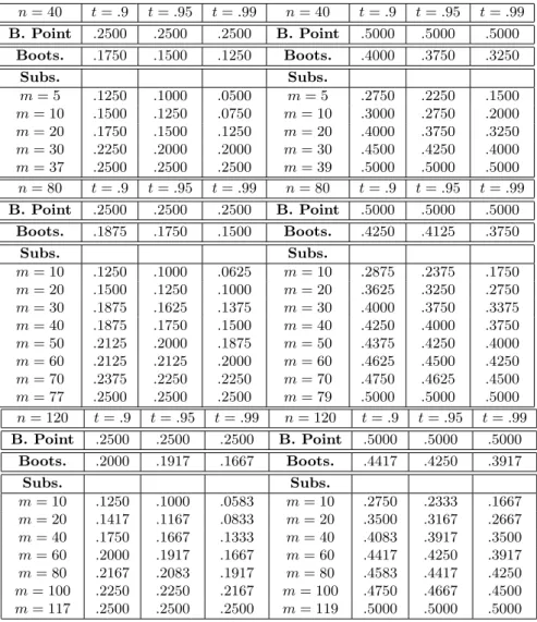
nontrivial breakdown point, to stay away from extreme quantiles, and to avoid small block sizes. Table 1.1 emphasizes this point by computing the subsampling quantile breakdown points whenn= 40,80,120, and for b = 0.25,0.5. The bootstrap quantile breakdown points based on Singh (1998) formula are often close to the ones given by medium subsample sizes.

Theorem 2 implies that we can always obtain a target upper quantile breakdown point ˆbt∈(1/n, b]

by selecting a suitable block size ˆmt=m(ˆbt). The formula for the smallest block size ensuring a given

upper breakdown point of subsampling quantiles is given below.

such that bt≥ˆbtis given by ˆ mt= inf n m:P h ˆ X(n, m,ˆbt−1/n)< mb i ≥t o ,

whereXˆ(n, m,ˆbt−1/n)is a hypergeometrically distributed random variable with parametersn,nˆbt−1,

andm.

Corollary 3 implies that for ˆbt = b it is possible to obtain a breakdown point bt as large as the

one of the statisticTn. As highlighted by Table 1.1, in order to achieve this goal it is not in general

necessary to select a trivial block sizem=n.

According to Theorem 2, the block size mhas to be sufficiently high, in order to avoid undesired subsampling breakdown properties. However to get consistency in a general setting a condition like m/n→0 should hold asn, m→ ∞(see, for instance, Politis, Romano and Wolf, 1999). This means that the application of Corollary 3 is essentially relevant to particular settings for which the consistency of the subsampling holds withm =O(n) (see Wu, 1990, and Remark 2.2.2 in Politis, Romano and Wolf, 1999).

The asymptotic subsampling breakdown behavior is characterized as follows.

Corollary 4 Let subsampling block size m satisfy m/n → r ∈ [0,1), m, n → ∞. Then, bt = b−

zt

p

b(1−b)(1−r)/√m+O(1/m), for n large enough, where zt is the t−quantile of the standard

normal distribution.

From Corollary 4, the subsampling breakdown pointbtconverges to the breakdown point of statistic

T as n, m→ ∞. Therefore, similar to the asymptotic bootstrap breakdown point formula in Singh (1998), Corollary 4 rules out the breakdown problem of subsampling quantiles for large samples and subsampling block sizes.

1.3.2

Breakdown Point and Data Driven Choice of the Block Size

A main issue in the application of subsampling procedures is the choice of block sizem, because the subsampling accuracy heavily depends on this parameter. In this section, we study the robustness of data driven block size selection procedures and derive the breakdown behavior of procedures based on either a minimization of the confidence interval volatility index (MCIV) or the calibration method (CM); see Romano and Wolf (2001). In particular, we are interested in computing the minimal proportion of contamination in the original sample such that the data driven choice of the block size fails and diverges to infinity. Letmu be the block size selected using MCIV or CM. We consider the

following definition for the breakdown point:

Definition 5 The breakdown point ofmu is defined as

bu

t := inf{p∈[1/n, p] :np∈N and mu=∞}, (1.3)

wherepis the fraction of observationsXi1, .., Xinp in original sample(X1, .., Xn)such thatXi1 → ±∞,

Xi2→ ±∞,. . . ,Xinp → ±∞.

In the next sections we briefly describe the MCIV and CM approaches, and compute their breakdown points.

Minimum Confidence Interval Volatility Method

A consistent method for a data driven choice of m determines the block size by minimizing the confidence interval volatility index across the admissible values of m. For brevity, we present the method for one–sided intervals. Modifications for the case with two–sided intervals are obvious.

Definition 6 Letmmin< mmaxandk∈Nbe fixed. Form∈ {mmin−k, .., mmin, .., mmax, .., mmax+k}

denote byQ∗

t(m)the (lower)t−subsampling quantile for block sizem. Further, defineQ

∗k

average quantile Q∗_tk(m) := 1 2k+ 1 j=k X j=−k Q∗

t(m+j). The confidence interval volatility (CIV) index is defined form∈

{mmin, mmin+ 1, ..., mmax−1, mmax} by

CIV(m) := 1 2k+ 1 j=k X j=−k ³ Q∗t(m+j)−Q ∗k t (m) ´2 . (1.4)

Let M := {mmin, mmin+ 1, . . . , mmax}. The data driven block size that minimizes the confidence

interval volatility index is

mv= arg infm∈M{CIV(m) :CIV(m)∈R+} , (1.5)

where, by definition, arg inf(∅) :=∞.

The block sizemvminimizes the empirical variance of the upper bound in a subsampling confidence

interval with nominal confidence level t. Typical recommended choices for k, mmin and mmax are

k = 2,3, mmin =c1nζ and mmax =c2nζ, respectively, where c1 ∈ [0.5,1], c2 ∈ [2,3] and ζ = 0.5;

see Romano and Wolf (2001). Moreoveor, according to Theorem 2, in order to ensure a minimal breakdown point for the quantile of the subsampling distribution, we can select the value ofmmin as

mmin= max(c1nζ,mˆt), (1.6)

where ˆmt is the minimal subsampling block size in Corollary 3, which ensures a breakdown point

larger than ˆbt.

Using Theorem 2, the formula for the breakdown point ofmv follows from Definition 5.

Corollary 7 For givent∈(0,1), let bt(m)be the subsampling upper t−quantile breakdown point in

Theorem 2, as a function of the block size m∈ M. Then we have: bv t = sup

Since mv is a crucial parameter for the accuracy of the resulting subsampling inference, it is

convenient to quantifybv

t for realistic applications. To this end, we can use Corollary 20. For instance,

for a sample sizen= 100 and for t= 0.99, we obtain mmin = 8 andmmax = 25, using the average

recommended choice in Romano and Wolf (2001), i.e., c1 = 0.75 and c2 = 2.5. For a statistic with

breakdown point b = 0.1 and for k = 3, this parameter setting implies bv

t = 0.03. In other words,

three outliers out of a hundred data points are sufficient to break down the data driven choice ofm based on the MCIV index.

Calibration Method

Another consistent method for a data driven choice of the block sizemcan be based on a calibration procedure in the spirit of Loh (1987). As above, we present this method for the case of a one–sided confidence interval only. The modifications for two-sided intervals are obvious.

Definition 8 Fix t∈(0,1) and let(X∗

1, . . . , Xn∗)be a bootstrap sample from (X1, . . . , Xn). For each

bootstrap sample, denote byQ∗∗

t (m)the t−sub-sampling quantile according to block sizem. The data

driven block size according to the calibration method is defined by

mc:= arg inf

m∈M{|t−P ∗_[T

n≤Q∗∗t (m)]|:P∗[Q∗∗t (m)∈R]>1−t}, (1.7)

where, by definition, arg inf(∅) := ∞, and P∗ _{denote the probability with respect to the bootstrap}

distribution.

By definition,mc is the block size for which the bootstrap probability of the event{Tn≤Q∗∗t (m)}

is as near as possible to the nominal level t of the confidence interval, but which at the same time ensures that the subsampling quantile breakdown probability of the calibration method is less thant. The last condition is necessary to ensure that the calibrated block sizemcdoes not imply a degenerate

subsampling quantileQ∗∗

t (mc) with a too large probability. By definition, the breakdown point ofmc

is the smallest fraction of outliers such that equation (2.12) is degenerate, similar to the MCIV index method. The formula for the breakdown point ofmc is given next.

Corollary 9 Lett∈(0,1). The breakdown point of mc is given by bct= max_m∈M{b∗∗t (m)},with

b∗∗t (m) = inf{p∈[1/n, b] :np∈Nand P[BIN(n, p)< nbt(m)]<1−t},

where bt(m) is for given m ∈ M the quantile subsampling breakdown point in Theorem 2 and

BIN(n, p) is a binomial random variable with parametersnandp.

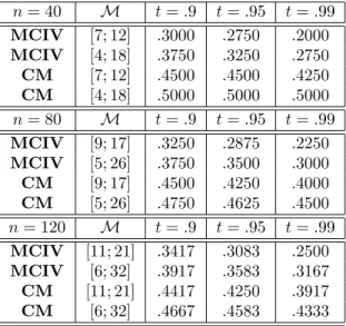
Table 1.2 compares the breakdown point ofmv andmc for some concrete parameter choices, given

a statistic with breakdown pointb= 0.5.

These theoretical results corroborated by unreported Monte Carlo results in linear regression mod-els indicate a higher robustness of the calibration method relative to the MCIV index method. There-fore, from a robustness perspective, the former should be preferred when consistent bootstrap methods are available. However, as discussed in Romano and Wolf (2001), the application of the calibration method in some settings can be computationally too expensive. In these cases, it is necessary to select an appropriate subset ofMfor the admissible block size (see Romano and Wolf (2001), Remark 5.4).

1.3.3

Robust Subsampling

To overcome the problem of the low breakdown point of subsampling quantiles, it is necessary first to apply subsampling methods to robust statistics, in order to avoid a trivial breakdown point from the beginning, and, second, to robustify the subsampling procedure itself. We first show how this goal can be achieved for the class of robust M-estimators, by applying the fast subsampling approach in Hong and Scaillet (2006). This approach, putted forward among others in Davidson and McKinnon

(1999) and Andrews (2002) in relation to the bootstrap, can be used to extend in a convenient way the robust bootstrap procedure for fixed point estimators in Salibian-Barrera, Van Aelst and Willems (2006, 2007) to the robust subsampling setting with M-estimators. In a second step, we study in more detail the linear regression setting, where explicit breakdown point characterizations are possible. We develop robust subsampling procedures for robust MM-estimators and derive a formula for the implied subsampling quantile breakdown point. These results are a natural complement to the theoretical findings obtained in Salibian-Barrera and Zamar (2002) for the robust bootstrap.

Let (X1, . . . , Xn) be an iid sample governed by the probability lawH. We consider the class of

robust M-estimators ˆθn for parameterθ∈Rd, defined by the solution of

ψn(ˆθn) = n

X

i=1

f(Xi,θˆn) = 0, (1.8)

for some functionψn:Rd→Rd depending on the parameterθand on the sample (X1, . . . , Xn).

Robust M−estimators typically have a bounded estimating function f. This feature is key for developing our robust subsampling approach in the M−estimation setting. As shown previously, a high breakdown point of ˆθn does not have to imply a high breakdown point for the corresponding

subsampling quantiles. For instance, in Table 1.1, we obtain very low breakdown points of subsampling quantiles, especially for small subsample sizes, even using robust estimators. A second issue is the fact that the application of robust estimators in resampling schemes can rapidly become prohibitive from a computational point of view.

To obtain a robust and computationally feasible subsampling method, we consider the following Taylor expansion of (1.8) around the true parameter value θ?: ψn(ˆθn) = ψn(θ?) +∇ψn(θ?)(ˆθn−

θ?) +oP(1), where∇ψn∈Rd×dis the matrix of partial derivatives with respect to parameterθ. This

implies: (ˆθn−θ?) = (−∇ψn(θ?))−1(ψn(θ?))+oP(1). Thus, we can consider: (−∇ψn(ˆθn))−1(ψn,m∗ (ˆθn))

as an approximation of ˆθ∗

Given the normalization constantτn, the robust subsampling distribution approximating the

sam-pling distribution ofτn(ˆθn−θ?) is defined by

LRn,m(x) = 1 Nn,m N_Xn,m s=1 I n τm(−∇ψn(ˆθn))−1(ψn,m,s∗ (ˆθn))≤x o , (1.9)

wheres indexes the set of possible subsamples,Nn,m=

¡_n

m

¢

, andI{·}is the indicator function. The following standard high-level assumptions ensures consistency of the robust subsampling for the class of robust M-estimators; see also Politis, Romano, and Wolf (1999).

(A1) ˆθn =θ?+OP(1/τn).

(A2) (−∇ψn(ˆθn))−1= (−∇ψn(θ?))−1+oP(1).

(A3) τn(ˆθn−θ?) = (−∇ψn(θ?))−1τn(ψn(θ?)) +oP(1).

(A4) There exists a limit law J(H) such that the distribution of τn(ˆθn−θ?) converges weakly to

J(H).

Given Assumptions (A1)-(A4), consistency of the robust subsampling scheme follows in the next theorem.

Theorem 10 Let Assumptions(A1)-(A4)be satisfied. Assume further thatτm/τn→0 andm/n→0

asm, n→ ∞. Then we get:

(1) Ifxis a continuity point of J(., H), then LR

n,m(x)→J(x, H)asn→ ∞.

(2) IfJ(., H)is continuous, thensupx|LRn,m(x)−J(x, H)| →0 in probability as n→ ∞.

(3) Given α ∈ (0,1) define cn,m(1−α) = inf{x : Ln,mR (x) ≥ 1−α} and c(1−α, H) = inf{x :

J(x, H)≥1−α}. IfJ(., H) is continuous atc(1−α, H), it then follows:

P

h

τn(ˆθn−θ?)≤cn,m(1−α)

i

Statements 1–3 in Theorem 10 are standard statements on the weak convergence of the robust sub-sampling approximation to the true asymptotic distributionJ(H) of√n(θbn−θ?). Statement 3 implies

that the (1−α)−quantile of Ln,mconverges to the corresponding (1−α)−quantile of J(H).

There-fore, the quantitiescn,m(1−α),α∈(0,1), can be used to construct finite sample tests and confidence

intervals forθ?.

Remark. The fast subsampling approach can be applied also with estimators ˜θn defined by the

solution of a set of smooth fixed-point equations gn(˜θn) = ˜θn, for some function gn : Rd → Rd

depending on the parameterθand the sample (X1, . . . , Xn). This follows from writing the fixed-point

equations in the form gn(˜θn)−θ˜n = 0. This corresponds to equation (1.8) with ψn = (gn −Id),

where Idis the identity function Id(x) = x. Consequently, in these cases the robust subsampling is equivalent to the extension of the robust bootstrap approach in Salibian-Barrera, Val Aelst and Willems (2007) to the subsampling setting.

In Section 1.3.4, we characterize explicitly the breakdown point of robust subsampling quantiles in the linear regression setting based on MM-estimates. More generally, we note from the robust subsam-pling definition (1.9) that the subsamsubsam-pling quantile breakdown point is maximal if: (i) (−∇ψn(ˆθn))−1

does not break down as long as ˆθn does not break down and (ii) given a subsampling block size m,

function ψ∗

n,m(ˆθn) is bounded with a bound that depends only on the original data set. The last

condition is typically satisfied by the estimating functions of robust M-estimators. The first one is often verifiable in concrete model settings.

1.3.4

Robust Subsampling in the Linear Regression Model

We consider the iid linear regression model:

where Yi is a scalar random variable,Xi an Rd−valued random variable,β ∈Rd, andσ∈R+. The

joint probability distribution of (Yi, Xi0)0 is denoted by H. Several robust estimators of β and σare

available in the literature; see, e.g., Hampel et al. (1986) for a review. We focus on a high-breakdown MM-estimator ofβ (Yohai, 1987).

Let{(yi, x0i)0:i= 1, .., n} be a sample of observations of model (1.10). The MM-estimateβbn ofβ

is defined by the implicit equation:

1 n n X i=1 ∇ρ1 Ã yi−x0iβbn b σn ! xi= 0. (1.11)

In equation (1.11), ∇ρ1 is the derivative of a continuously differentiable, bounded and symmetric

functionρ1, satisfying the assumption (A1)-(A4) below. σbnis a scaleS−estimate that minimizes with

respect toβthe M−estimatebσn(β), defined implicitly by 1

n n X i=1 ρ0 µ yi−x0iβ b σn(β) ¶ =B,where functionρ0

satisfies the same assumptions asρ1andB is a positive constant. We denote by ˜βn theS−regression

estimate, i.e.,σbn=bσn( ˜βn). The choice ofBdetermines the breakdown point of the estimators, which

is maximal forB= 0.5 (see, e.g., Huber, 1981).

To define the robust subsampling for the linear regression setting we introduce the following no-tation.

Notation 11 (i) For i = 1, .., n, define the residuals: bri = yi −x0iβbn and r˜i = yi−x0iβ˜n, and

compute the weights: ωbi =∇ρ1(bri/σbn)/bri,v˜i = bσn

nBρ0(˜ri/bσn)/r˜i. (ii) Given m < n, define for every subsampling block {(y∗

i, x∗i0) :i = 1, .., m} the residuals bri∗ =yi∗−xi∗0βbn and r˜∗i = y∗i −x∗i0β˜n, and

compute the weights:

b ω∗ i =∇ρ1(rbi∗/bσn)/br∗i, v˜i∗= b σn nBρ0(˜r ∗ i/bσn)/r˜∗i. (1.12)

With these weights, define: b β∗ n,m= Ã_m X i=1 b ω∗ ix∗ix∗i0 !−1 _m X i=1 b ω∗ ix∗iyi∗, bσn,m∗ = m X i=1 ˜ v∗ i(yi∗−x∗i0β˜n). (1.13)

In equation (1.12), the weights bω∗

i and ˜vi∗ are computed without recalculating the estimators βbn,

˜

βn and bσn in each subsampling block. The same applies to the quantities βbn,m∗ and bσ∗n,m in (1.13),

which are therefore only an approximation of the “true” point estimatesβb∗

m andbσ∗mimplied by the

subsampling block {(y∗

i, x∗0i ) :i = 1, .., m}. Following the insight of the previous section, the basic

idea is to correct for the asymptotic bias between (βb∗0

n,m,σb∗n,m) and (βb∗0m,bσm∗) using a first-order linear

correction that depends only on βbn, ˜βn and bσn. In this way, the large breakdown point of these

estimators will be inherited by the implied subsampling quantiles. Moreover, since it is not necessary to compute in each subsampling block the implied robust point estimate, the robust subsampling in Definition 12 yields a computationally feasible resampling scheme, which allows us to compute robust confidence intervals for regression parameterβ in presence of nuisance scale parameterσ.

Definition 12 Let β? be the true parameter value in the regression model (1.10) and Jn(H) be the

sampling distribution of √n(βbn−β?), i.e., for any x∈Rn: Jn(x, H) =P

h_√

n(βbn−β?)≤x

i

. The robust subsampling approximation ofJn(x, H)is given by

LRn,m(x) = 1 Nn,m N_Xn,m s=1 I n Mn √ m(βb∗n,m,s−βbn) +dn √ m(σb∗n,m,s−bσn)≤x o , (1.14)

where the linear correctionsMn anddn are defined as follows: Mn = bσn à _n X i=1 ∇2_ρ 1(bri/σbn)xix0i !−1 _n X i=1 b ωixix0i, dn = nB b σ2 n n X i=1 ∇ρ0(˜ri/σbn)˜ri/σbn à _n X i=1 ∇2_ρ 1(bri/bσn)xix0i !−1 _n X i=1 ∇2_ρ 1(bri/σbn)brixi.

The following are detailed assumptions on the robust linear regression setting based on the above MM-estimator, which ensure consistency of the robust subsampling approximation in Definition 12.

(A5) The sampling distributionJn(H) converges weakly to a limit distributionJ(H) asn→ ∞.

(A6) The following limits in probability hold asn→ ∞: βbn→β?, ˜βn→β˜?,σbn→σ?, where parameters

β?,β˜?andσ?are the unique solution of the set of moment conditions: E[∇ρ1((Y1−X10β)/σ)] =

0, Ehρ0((Y1−X10β˜)/σ) i =B,Eh∇ρ0((Y1−X10β˜)/σ) i = 0.

(A7) For j = 0,1, the function ρj is three times continuously differentiable and such that: (R1)

ρj(−u) = ρj(u) for all u ∈ R; (R2) ρj(0) = 0; (R3) supu|ρj(u)| = 1; (R4) If ρj(u) <1 and

0< v < uthenρj(v)< ρj(u).

(A8) Letr=Y1−X10β?. The following expectations exist:

E · ∇ρ1(r) r X1X 0 1 ¸ , E[∇ρ1(r)X1X10], E £ ∇2_ρ 1(r)X1X10 ¤ , E[∇ρ1(r)rX1X10], (1.15) E · ∇ρ0(r) r X1X 0 1 ¸ , E[∇ρ0(r)r], E £ ∇2_ρ 0(r)X1X10 ¤ , (1.16) E£∇2ρ0(r)rX1 ¤ , E£∇2ρ1(r)rX1 ¤ .

In addition, the first and the third matrices in (1.15) and in (1.16) are invertible, and the second expectation in (1.16) is not zero.

(A9) The following functions are continuous: u7−→ ∇ρ0(u) u , u7−→ ∇ρ0(u)− ∇2ρ0(u)u u2 , u7−→ ∇ρ1(u)− ∇2ρ1(u)u u2 .

Consistency of the robust subsampling in Definition 12 is stated in the next theorem.

Theorem 13 Let Assumption(A5)-(A9) be satisfied. Then we get:

1. If xis a continuity point of J(·, H), then the following limit in probability holds as n, m→ ∞

andm/n→0: LR

n,m(x)→J(x, H).

2. IfJ(·, H)is continuous, then the following limit in probability holds asn, m→ ∞andm/n→0: sup

x |L R

n,m(x)−J(x, H)| →0.

3. Forα∈(0,1), define cn,m(1−α) = inf{x:LRn,m(x)≥1−α}, c(1−α, H) = inf{x:J(x, H)≥

1−α}. IfJ(·, H)is continuous atc(1−α, H), then the following limit holds asn, m→ ∞and m/n→0: Ph√n(βbn−β?)≤cn,m(1−α)

i

→1−α.

In contrast to the general M-estimator case, we can exploit the additional structure of the linear regression setting to explicitly characterize the breakdown point of robust subsampling quantiles. The breakdown point formula for the robust subsampling in Definition 12 is given in the next theorem.

Theorem 14 Let√bω1x1, ..,

√

b

ωnxn be in general position, i.e., any drow vectors of then×ddesign

matrixX = [√ωbix0i]i=1,..,n are linearly independent, and fix t∈(0,1).

1. The breakdown pointbR

t of thet−quantile of the robust subsampling in Definition 12 is given by

bR

whereX(n, m, p)is a hypergeometrically distributed random variable with parametersn,np, and m, andb is the breakdown point of the robust M M−regression estimatorβbn.

2. LetbbR

t ∈(1/n, b]be such that nbbRt ∈N. The smallest block size mbRt such that bRt ≥bbRt is given

by b mRt = inf{m:P h b X(n, m,bbRt −1/n)≤m−d i ≥t}, whereXb(n, m,bbR

t −1/n)is a hypergeometrically distributed random variable with parameters n,

nbbR

t −1, andm.

The assumption on the general position of√ωb1x1, ..,

√

b

ωnxnis also used in Salibian-Barrera and Zamar

(2002), and is needed here to ensure that the approximation βb∗

n,m of the subsampling estimate βb∗m

is well-defined in every subsampling block. By comparing (1.17) with the breakdown formula (1.2) of the standard subsampling in Theorem 2, we note that for reasonable parameter choices mb << m−d = m(1−d/m). Therefore, P[X(n, m, p)< mb] << P[X(n, m, p)≤m−d] and bR

t >> bt.

The numerical difference between the two breakdown points can be large. Table 1.3 computes the robust subsampling breakdown point for a setting withd= 3 and for sample sizesn= 40,80,120, in dependence of the breakdown pointbof theM M−regression estimatorβbn. We find that statement 2

of Theorem 14 can be more relevant for applications than the one of Corollary 3. This is so because a large breakdown point of the robust subsampling can arise also for small subsampling block sizes, which asymptotically can more easily ensure the subsampling consistency conditions.

For b= 0.225 andn= 40, the robust subsampling breakdown point isbR

t = 0.225 for allm≥6.

Fort= 0.9, the maximal breakdown point is obtained already form= 8. Fort= 0.95 andt= 0.99, it is obtained form= 10 andm= 12, respectively. In general, the maximal breakdown point is obtained for all samples sizes and confidence levels in Table 1.3, independently ofb, form= 14. Whenb <0.5,

the value ofmensuring the maximal breakdown point is even lower. These are large differences with respect to the subsampling breakdown points in Table 1.1.

These results have implications also for the breakdown point ofmv in Corollary 20. For instance,

with a sample size n = 100, the average recommended choice in Romano and Wolf (2001) yields mmin= 8 andmmax= 25 (usingc1= 0.75 andc2= 2.5). Forb= 0.1 andk= 3, the breakdown point

ofmvwhen using the robust subsampling is maximal for all confidence levels, but the one when using

the standard subsampling is bv

t = 0.03 fort= 0.99. On the other side, the breakdown point ofmc is

much higher, as was shown by our previous numerical computations.

Remark. Our results on the robust subsampling extend directly to linear regression models with fixed designs. Assume that the covariates Xi ∈ Rd are fixed and part of an infinite sequence

(X1, . . . , Xn, Xn+1, . . .). For Zi = (Yi, Xi0)0, let H be the joint probability law governing the

infi-nite sequence (Z1, . . . , Zn, Zn+1, . . .). Salibian-Barrera (2006a) proves consistency and asymptotic

normality of MM-estimators in this setting. Moreover, Salibian-Barrera (2006b) shows the validity of the first order Taylor expansion for the corresponding fixed-point estimating equation. Under the weak assumptions of Theorem 4.3.1 in Politis, Romano and Wolf (1999), the consistency of the robust subsampling in Definition 1.14 then follows even for settings with fixed designs.

1.4

Monte Carlo Study and Sensitivity Analysis

We study through Monte Carlo simulations the statistical properties of the subsampling and the robust subsampling in estimating (i) the distribution of the square of the sample average for an iid normal sample and (ii) the confidence interval of a parameter of interest in an iid linear regression model (1.10) when this parameter is possibly near a boundary. In both settings, the bootstrap is inconsistent, but subsampling procedures are applicable.

1.4.1

Square of the Sample Average

The first example considers the sampling distribution of the square of the sample average based in an iid normal sample. This is an informative, albeit simple, design to measure the accuracy of the subsampling in presence of model contaminations. As discussed, e.g., in Datta (1995), the bootstrap fails in this setting and only a modified bootstrap procedure is applicable. Instead, the subsampling is consistent without modifications of the standard procedure.

Model and Estimation

Let (X1, . . . , Xn) be an iid sample withXi∼N(µ, σ2), where µ= 0 andσ2= 1, and ¯Xn =

1 n n X i=1 Xi

be the sample average. Using subsampling, we estimate the distribution of n¡( ¯Xn)2−µ2

¢

. Let (X∗

1, . . . , Xm∗) be a random subsample and ¯Xn,m∗ =

1 m m X i=1 X∗

i be the subsample average. Then, the

subsampling distribution approximation reads:

LN Rn,m(x) = 1 Nn,m N_Xn,m s=1 I©m(( ¯Xn,m,s∗ )2−( ¯Xn)2)≤x ª . (1.18)

For the robust subsampling, we consider the robust location estimate ¯XR

n given as solution of the

equationψn( ¯XnR) = 0, where functionψn is defined by

ψn(θ) = 1 n n X i=1 hc(Xi−θ), (1.19)

andhc(x) =x·min(1, c/|x|) is the Huber function. To estimate the distribution ofn

¡

( ¯XR n)2−µ2

¢

, we start by considering the subsample statisticm(( ¯XR∗

n )2−( ¯XnR)2) =m(( ¯XnR∗−X¯nR)2+2 ¯XnR( ¯XnR∗−X¯nR)),

where ¯XR∗

n is the subsample robust estimate of µ. This approximation does not directly generate a

robust subsampling distribution. Therefore, in the last expression we use our robust subsampling approach to estimate the distribution of ( ¯XR∗

of the distribution ofn(( ¯XR n)2−µ2) is defined by LR n,m(x) = 1 Nn,m N_Xn,m s=1 I©m((An,m,s)2+ 2( ¯XnR)(An,m,s))≤x ª , (1.20) whereAn,m,s= (−∇ψn( ¯XnR))−1ψn,m,s∗ ( ¯XnR). Numerical Results

We consider sample sizes n = 40,80,120. Since the calibration method is not applicable here, we use a data driven block size obtained by minimizing the CIV index for k = 2. For sample sizes n = 40,80,120, the average recommended choice in Romano and Wolf (2001) implies a lower and upper boundmmin= 5,7,8 andmmax= 16,22,27 forc1= 0.75 andc2= 2.5, respectively.

We study the finite sample coverage implied by the classical and robust subsampling methods. To this end, we test the null hypothesis H0 : (µ?)2 = 0 against H1 : (µ?)2 >0, under a contaminated

normal distribution forXi:

Xi∼(1−γ)N(0,1) + γ

2(N(5,100) +N(−5,100)),

forγ= 0 (no contamination),γ= 0.05 (5% of contaminated data) andγ= 0.10 (10% of contaminated data). For each of the 2000 Monte Carlo replications, subsampling distributions are computed based on 500 draws. Tables 1.4 summarizes the empirical frequencies of non rejection of null hypothesisH0

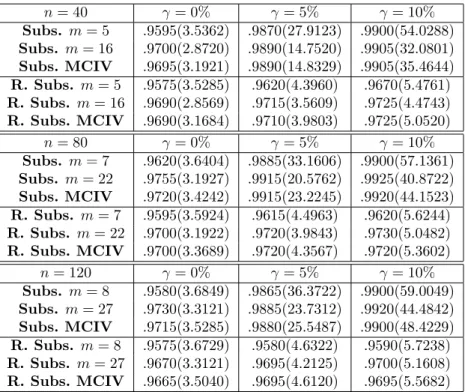
for a confidence level 1−α=.95. In all Monte Carlo simulation settings, we find that the empirical frequencies for the robust subsampling are quite accurate and closer to the nominal frequencies than those of the classical subsampling. Under a model contamination, the underrejection of the null hypothesis using classical subsampling methods can be severe. For all sample sizes we get an empirical rejection frequency of .99 instead of the true .95 value when γ = 0.10. At the same time, the

one-sided confidence interval implied by the subsampling virtually explodes in presence of contamination, leading to a virtually non informative inference. For instance, whenγ= 0.10 andn= 120, the median .95-quantile implied by the subsampling approximation is 48.42 while the one implied by the robust subsampling approximation is 5.56.

1.4.2

Linear Regression

In this section we consider the iid linear regression model (1.10) when a parameter of interest is possibly near a boundary (see, e.g., Kim, Stone and White (2005) for an application in finance). As discussed in detail by Andrews (2000), the bootstrap is inconsistent in this context and the subsampling is a potentially natural alternative to it. Moreover, Andrews and Guggenberger (2009a, 2010a,b) (see also Mikusheva (2007) for a similar problem in autoregressive models with unit roots) show that pure subsampling methods have a lack of uniform asymptotic approximation within a class of models including our Monte Carlo setting. They also develop hybrid and size-correction procedures to fix the arising asymptotic size distortion. Analogous remarks hold in the linear regression model when making inference on a parameter of a given regressor and the parameter of another regressor, a nuisance parameter, may be near a boundary. We follow their hybrid approach in our Monte Carlo study of the classic and robust subsampling.

Model and Estimation

We consider the regression parameterβ ∈R, which is known to satisfy the constraintβ≥0 in the iid linear regression model:

Yi = Xi0θ+Wiβ+σUi,

= Z0

where Yi, Wi are scalar, Xi is anRd−1-valued random variable,θ ∈Rd−1, and σ ∈R+. Moreover,

Zi(1) =Xi(1) = 1,η(1)=θ(1),Zi(2)=Wi,η(2)=β and for 3≤j ≤d, Zi(j) =Xi(j−1), η(j)=θ(j−1),

where h(j) denotes the j-th coordinate of vector h. The common joint distribution of (Yi, Zi0)0 is

denoted by H. Let{(yi, zi0)0 : i = 1. . . , n} be a sample of observations of model (1.21). In order

to construct confidence intervals for parameter β using the classic subsampling, we consider the constrained estimator ˆβN R

n = max(0,ηˆnols(2)), where ˆηolsn is the (unrestricted) OLS estimator of η. For

the robust subsampling, we consider the constrained estimator ˆβR

n = max(0,ηˆnrob(2)), where ˆηnrob is a

MM-estimator of η. The S-estimate ˆσn = ˆσn(˜ηnrob) is computed from a constrained robust estimator

˜ ηrob

n ofη under the constraintη(2) ≥0.

Given subsampling blocks{(y∗

i, z0∗i )0 :i= 1, . . . , m}, we construct consistent subsampling and

ro-bust subsampling methods as follows. For the subsampling, we compute in each block the constrained estimator ˆβN R

n,m= max(0,ηˆolsn,m(2)). The subsampling distribution function estimating the distribution

function of√n( ˆβN R n −β?) is then given by LN R n,m(x) = 1 Nn,m N_Xn,m s=1 In√m( ˆβN R n,m,s−βˆnN R)≤x o . (1.22)

For the robust subsampling, we follow (1.13) and (1.14) and additionally account for the parameter constraint. Thus, we consider the robust subsampling statistic:

ˆ

subβ∗n,m = max

³

(Mn(ˆη∗n,m−ηˆrobn ) +dn(ˆσn,m∗ −σˆn))(2)+ ˆβnR,0

´

. The robust subsampling distribu-tion funcdistribu-tion which approximates the distribudistribu-tion funcdistribu-tion of√n( ˆβR

n −β?) is then given by LR n,m(x) = 1 Nn,m N_Xn,m s=1 In√m( ˆsubβ∗_n,m,s−βˆR n)≤x o . (1.23)

By construction, the theoretical results in Section 1.3.4 for the upper quantile breakdown of the robust subsampling distribution in Definition 12 hold also for (1.23).

Hybrid Procedures

Using (1.22) and (1.23), we construct hybrid, classical and robust, equal-tailed confidence intervals for parameterβ as follows. Letcn,m(1−α) be the (1−α)-quantile implied by either (1.22) or (1.23).

The corresponding hybrid quantile is:

cH

n,m(1−α) = max(cn,m(1−α), c∞(1−α)), (1.24)

where c∞(1−α) is the quantile of the asymptotic distribution of

√

n( ˆβi

n−β?), i =CL, R, for the

unconstrained, either classical or robust, estimator ˆβi

n of β. To compute c∞(1−α), one can use

standard asymptotic normality results for OLS estimators and the asymptotic normality results for MM-estimates in Yohai (1987). However, Salibian-Barrera and Zamar (2002) show that these asymp-totic approximations behave poorly in presence of contamination. Therefore, we use the bootstrap and the robust bootstrap, for the subsampling and the robust subsampling, respectively, to estimate the distribution of the unconstrained estimators in the computation of hybrid quantiles. Unreported numerical results confirm the superiority of this approach. In this way, the construction of hybrid quantiles for our robust subsampling approach can profit also from the robustness properties of the robust bootstrap developed in Salibian-Barrera and Zamar (2002).

Numerical Results

We consider the iid linear regression model (1.21) for d= 3,5. The true parameter vector is η? =

(0, β?,0)0 and η? = (0, β?,0,0,0)0, respectively, with β? = 0.25, which is a parameter value near to

the boundary 0. Since the calibration method is not applicable here, we use a data driven block size obtained by minimizing the CIV index with k = 2. For our sample sizes n = 40,60, the average recommended choice in Romano and Wolf (2001) implies an upper bound mmax = 16, mmax =

19 for c2 = 2.5 respectively. For the lower bound, we apply equation (1.6) in order to obtain a

breakdown point of at least 40% for the 0.975 quantile. This implies mmin ≥ 9,13 for d = 3,5,

respectively, restricting the standard choice of mmin, especially for d = 5. In order to allow for a

non trivial data-driven block size selection whend = 5, we then set mmax = 18,23 in this case for

n= 40.60, respectively. We make use of functionsρ0 andρ1 in Tukey’s family. The constant for the

M M−regression estimator in our simulations is B = 0.5. For this choice, we obtain a breakdown point ofηbn satisfyingb≥0.47; see Yohai (1987, Theorem 2.1).

We first study the finite sample coverage implied by classical and robust subsampling methods. To this end, we test the null hypothesisH0:β?= 0.25 under a contaminated normal distribution for

U:

U ∼(1−γ)N(0,1) + γ

2(N(C,(0.1)

2_{) +N(−C,(0.1)}2_{)), (1.25)}

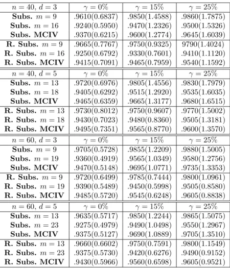
where C = 5, γ = 0 (no contamination), γ = 0.15 (15% of contaminated data) andγ = 0.25 (25% of contaminated data), as in Salibian-Barrera and Zamar (2002). For each of the 2000 Monte Carlo replications, subsampling distributions are based on 200 draws. Tables 1.5 summarizes the empirical frequencies of non rejection of null hypothesisH0and the median confidence interval lengths for the

confidence level 1−α=.95.

In all Monte Carlo simulation settings, the empirical frequencies for the robust subsampling with data driven choice of the block size are quite accurate and closer to the nominal frequencies than those of the classical subsampling. Unreported results for the inconsistent bootstrap and robust bootstrap yield empirical rejection frequencies between 67.5% to 72.3%. Similarly, the subsampling and robust subsampling without hybrid correction yield empirical frequencies between 60.1% and 65.4%, which are not too far away from the theoretical distorted asymptotic size (1−α)/2 of equal-tailed confi-dence intervals; see Andrews and Guggenberger, 2010b. Unreported results for the parameter choice

β? = 0.1 show that the undercoverage of inconsistent procedures is, as expected, larger, while hybrid

robust methods maintain an accurate coverage. Results of the robust bootstrap and hybrid robust subsampling for the parameter choice β? = 0.5 are more similar, as expected, but still in favour of

the latter. Unreported results with different contamination sizes, model dimensions and sample sizes (e.g.,C= 4 , d= 20) produced similar results.

The median length of the robust subsampling confidence intervals is moderately higher in the setting with no contamination (γ = 0%). For instance, for the case n = 40, d = 3, the median confidence interval of the robust subsampling is approximately 14% higher than the median length of the subsampling. However, in presence of contamination the robust subsampling produces clearly more efficient inferences with dramatically smaller median confidence interval lengths. For instance, for the casen= 40,d= 3, the median confidence interval of the robust subsamppling is approximately 38% (28%) lower than the median length of the subsampling when γ = 15% (γ = 25%). These are large differences having obvious implications for the power of tests based on subsampling and robust subsampling methods.

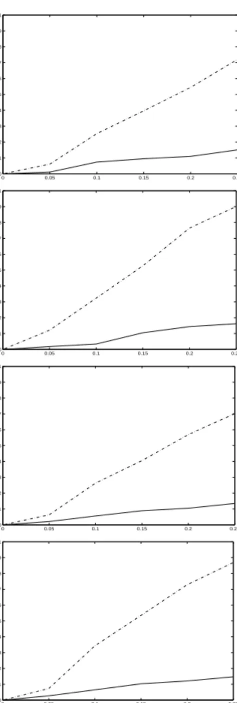
We have also studied the sensitivity of the subsampling and robust subsampling inference with respect to empirical contaminations of the data. For each Monte Carlo sample, let:

Ymax= arg max

Y1,...,Yn

{u(Yi)|u(Yi) =Yi−Zi0η,underH0}, (1.26)

We modifyYmax over a grid within the interval [Ymax+ 1, Ymax+ 4]. Then, we analyze the sensitivity

of the resulting empirical averages ofp-values for testing the null hypothesisH0 :β? = 0.25. Figure

1.1 summarizes the results.

As expected, we obtain quite large absolute variations in averagep-values for the subsampling and an almost flat sensitivity curve for the robust subsampling.

under H0:β? = 0.25, with increasing contamination sizes γ∈[0,0.25] in (1.25), and have analyzed

the averagep−value variation with respect to the setting with no contamination (γ= 0). Figure 1.2 summarizes the results.

Also in this case, the subsampling clearly implies larger variations in averagep-values as a function of the size of contamination in the data, indicating the fragility of the implied inference results.

1.5

Conclusions

We derive a formula for the breakdown point of subsampling quantiles, which is shown to imply fragile subsampling procedures for moderate block sizes, even when subsampling is applied to robust statistics. This instability is inherited by data driven block size selection procedures. We propose consistent robust subsampling methods for the class of M-estimators and derive detailed breakdown point formulas for MM-estimators in the linear regression setting. Monte Carlo simulations in two settings where the bootstrap is known to fail show the usefulness of robust subsampling relative to the classical subsampling for producing accurate inferences in presence of model deviations.

A.1 Proofs

Proof of Theorem 2. The quantile Q∗

t breaks down if and only if the proportion of bounded

realizations of the statisticT∗

n,mis less thant, i.e., when the proportion of subsamples with less than

mboutliers is less thant. LetX(n, m, p) be the number of outliers in subsample (X∗

1, . . . , Xm∗), when

np is the number of outliers in the original sample (X1, . . . , Xn). The random variable X(n, m, p)

follows a hypergeometric distribution with parametersn,np, andm. Consequently,btis the smallest

proportionpsuch thatnp∈andP[X(n, m, p)< mb]< t, which is the stated result.

Proof of Corollary 3. Existence of ˆmt is ensured by Theorem 2. For a hypergeometrically

distributed variable X(n, m, p) such that np ∈, the probability P[X(n, m, p)< mb] is decreasing in p. Therefore,bt( ˆmt)≥ˆbt. By definition, for every integerm <mˆt,P

h

ˆ

X(n, m,ˆbt−1/n)< mb

i

< t, andbt(m)≤ˆbt−1/n. This concludes the proof.

Proof of Corollary 4. Let us takep=b−zt

p

b(1−b)(1−r)/√m+c/m, forp∈[0, b], and compute a Berry-Esseen type bound for the normal approximation of the hypergeometric distribution, where c is in a fixed compact set. Forn and c large enough,P[X(n, m, p)< mb]< t, whereX(n, m, p) is a hypergeometric random variable with parameters n, np, and m. Forn large enough and c small enough,P[X(n, m, p)< mb]> t. Therefore,bt=b−zt

p

b(1−b)(1−r)/√m+O(1/m), as stated. Proof of Corollary 20. By definition, in order to get mv =∞we must have CIV(m) =∞for

all m ∈ M. Given m ∈ M, CIV(m) = ∞ if and only if the fraction of outliers p in the sample

{X1, . . . , Xn} satisfiesp≥min{bt(m−k), bt(m−k+ 1), .., bt(m+k−1), bt(m+k)}. This concludes

Proof of Corollary 22. By definition, in order to get mc=∞we must haveP[Q∗∗t (m) =∞]≥t

for all m∈ M. Q∗∗

t (m) =∞ if the number of outliers in bootstrap sample (X1∗, . . . , Xn∗) is at least

as large as nbt(m). The number of outliers in the bootstrap sample is distributed as B(n, p). This

concludes the proof.

Proof of Theorem 10. Under Assumptions (A1)-(A4) the statements of the theorem follow from Theorem 1 in Hong and Scaillet (2006).

Proof of Theorem 13. We first rewrite the estimatorτn = (βbn0,bσn,β˜n0)0 as the fixed point of the

following system of equations:

b βn = An(βbn,bσn)−1Vn(βbn,bσn), b σn = σbnUn( ˜βn,σbn), ˜ βn = Bn( ˜βn,bσn)−1Wn( ˜βn,σbn), (1.27) where An(β, σ) = 1 n n X i=1 ∇ρ1((yi−x0iβ)/σ) yi−x0iβ xix0i, Vn(β, σ) = 1 n n X i=1 ∇ρ1((yi−x0iβ)/σ) yi−x0iβ yixi, Un( ˜β, σ) = 1 n n X i=1 ρ0((yi−β˜0xi)/σ) B(yi−β˜0xi) (yi−β˜0xi),

an