Design and Optimization of Passive Wireless Intraocular Pressure Sensor.

(1)

ABSTRACT

KATURI, KALYAN CHAKRAVARTHI. Design and Optimization of Passive Wireless Intraocular Pressure Sensor. (Under the direction of Melur K. Ramasubramanian.)

Glaucoma diagnosis and the prevention of the disease progression depend heavily on

the accuracy of intraocular pressure measurements. Continuous monitoring of intraocular

pressure would make it possible to arrest the disease progression early so that the patient

does not lose much of his vision. The objective of this research is to develop a design process

for a minimally invasive implantable sensor for continuous intraocular pressure monitoring.

The design process include identification of optimal implant location, estimation of available

space for the implant, MEMS pressure sensor design, magnetic link design, and optimal

implant insertion method. As a part of the pressure sensor design cycle, a micro scale

capacitive pressure sensor was designed, fabricated and tested. Kapton and ParyleneC

based flexible implant fabrication processes were investigated to develop sensor implant

that could be inserted in a minimally invasive manner. An implant delivery system was

designed for inserting the implant using incision sizes of 2.8mm-3mm on the corneal surface.

A finite element analysis of the insertion process was modeled to identify stress concentration

regions in the implant and for determining the orientation of implant in the delivery device

(2)

(3)

Design and Optimization of Passive Wireless Intraocular Pressure Sensor

by

Kalyan Chakravarthi Katuri

A dissertation submitted to the Graduate Faculty of North Carolina State University

in partial fulfillment of the requirements for the Degree of

Doctor of Philosophy

Mechanical Engineering

Raleigh, North Carolina

2012

APPROVED BY:

Gianluca Lazzi Larry M. Silverberg

(4)

DEDICATION

(5)

BIOGRAPHY

The author was born in a small town in the coastal region of Andhra Pradesh, India. After

finishing his bachelors in mechanical engineering from Jawaharlal Nehru Technological

University in Hyderabad, he enrolled as an MS graduate student at NC State. After finishing

his Masters degree (concentration:Mechatronics) in 2006, he enrolled as a PhD student in

mechanical engineering department at NC State. Kalyan’s research interests include applied

mechanics, controls and instrumentation, computational mechanics, wireless passive sensor

(6)

ACKNOWLEDGEMENTS

First and foremost I offer my gratitude to my advisor, Dr Ramasubramanian, who has

sup-ported me throughout my Masters and PhD. He patiently allowed me to work in my own way.

He never shot down my wild research ideas. Instead, he encouraged me to pursue them to

see if they work. Whenever I was about to go off on a tangent from my main research topic,

he would gently steer me back onto the right course. His passion for applied mechanics and

biomimetic systems has been very inspiring to me and helped me shape my own research

interests. I could not ask for a better teacher.

I also would like to thank Dr.Lazzi, Dr.Roberts, and Dr.Silverberg for their time and

support. Dr. Sanjay Asrani of Duke university has offered me much needed advice and

insight on intraocular pressure sensing design constraints. I thank Dr. Mark Walters and Kirk

Bryson of Duke university for training me on cleanroom equipment. Thanks to Dr. Ginger Yu

for helping me test MEMS pressure sensors.

A special thanks to Dr. Xiaoning Jiang and his PhD student Kim for giving me access to

the impedance analyzer in their lab and for helping me get started on it. Thanks to Lance C.

Mangum for installing Coventorware software on the lab server. None of this would have

been possible without the guidance of the above-mentioned people and without the support

of my research group: Sameer Tendulkar, Swapnil Gupta, and Guang Chen.

Finally, I would like to thank my parents, my sister, my brother-in-law and my friends:

Siddharth Patel, Abhishek Raina, Amol Ghonge, and Kiran Kumar Kethineedi for their love

(7)

LIST OF TABLES

Table 1.1 Summary of coil based (wireless) design specifications . . . 13

Table 1.2 Non-telemetry Techniques . . . 14

Table 2.1 Coil Geometrical Design Parameters . . . 25

Table 3.1 Reader Coil Impedance Design Parameters . . . 31

Table 3.2 Design Parameters . . . 33

Table 3.3 Movable electrode plate deflection . . . 37

Table 3.4 Capacitor combinations . . . 44

Table 3.5 Capacitance measured at Atmospheric Pressure, 8mins etch time . . . 44

Table 3.6 Capacitance measured at Atmospheric Pressure, 12mins etch time . . . . 45

Table 4.1 Sensor implant pressure sensitivity . . . 68

(10)

LIST OF FIGURES

Figure 1.1 Aqueous humor flow path in a healthy eye[3]. . . 2

Figure 1.2 Open-angle and angle-closure glaucoma[6]. . . 4

1.2.1 Open-angle glaucoma. . . 4

1.2.2 Angle-closure glaucoma. . . 4

Figure 1.3 IOP measurement techniques classification . . . 7

Figure 2.1 In vivo cross-sectional view of a live human eye anterior segment obtained using optical coherence tomography. . . 24

Figure 2.2 An illustration of implant location on top of iris inside the anterior chamber . . . 24

Figure 3.1 Time domain lumped parameter model of passive IOP sensor . . . 27

Figure 3.2 Frequency domain lumped parameter model of passive IOP sensor . . 27

Figure 3.3 Skin depth of Copper and Gold . . . 28

Figure 3.4 Reader coil phase . . . 32

Figure 3.5 Reader coil amplitude . . . 33

Figure 3.6 Effect of Q factor on impedance phase dip . . . 34

Figure 3.7 Finite element model of MEMS pressure sensor[9]. . . 35

Figure 3.8 Stress distribution in a 100µm×100µm cap sensor at a pressure load of 50mmHg above atmospheric pressure[9]. . . 36

Figure 3.9 MEMS capacitive sensor fabrication step sequence[9] . . . 38

3.9.1 . . . 38

3.9.2 . . . 38

3.9.3 . . . 38

3.9.4 . . . 38

3.9.5 . . . 38

3.9.6 . . . 38

3.9.7 . . . 38

3.9.8 . . . 38

3.9.9 . . . 38

3.9.10 . . . 38

Figure 3.10 MEMS capacitive sensor after the removal of sacrificial oxide . . . 39

Figure 3.11 Poly0 line after HF etch . . . 41

Figure 3.12 SEM image of released sensors[9] . . . 42

Figure 3.13 Capacitive pressure sensors with etch channels in the side walls.[9] . . 43

Figure 3.14 Parallel MEMS capacitive sensors[9] . . . 43

(11)

Figure 3.16 12 minute etch spectra. The oxide count is found to be statistically

insignificant . . . 45

Figure 4.1 A multi-coil based pressure sensor . . . 49

Figure 4.2 Lumped parameter equivalent circuit of multicoil based sensor[1] . . . 49

Figure 4.3 Spiral inductor circuit model . . . 50

Figure 4.4 Fabrication process flow of Kapton based IOP sensor implant . . . 54

Figure 4.5 Cross-sectional view of Kapton based IOP sensor . . . 55

Figure 4.6 Coils made using screen printing technique . . . 55

Figure 4.7 Radius estimates for differnt values of maximum applied pressure . . . 58

Figure 4.8 Kapton diaphragm, 250 microns radius . . . 59

4.8.1 Deflection of 4micron thick Kapton diaphragm. . . 59

4.8.2 Radial pattern on Copper to lower bending stiffness. . . 59

4.8.3 Deflection of 4micron thick grooved Kapton diaphragm. . . 59

Figure 4.9 Capacitance Vs Pressure of Kapton pressure sensor of 600µm radius . . 60

4.9.1 Kapton 4micron thick, 600microns radius . . . 60

4.9.2 Kapton 12micron thick, 600microns radius . . . 60

Figure 4.10 Mode shapes and frequencies of 600 micron Kapton Sensor . . . 61

Figure 4.11 Effect of in-plane residual stress on sensor performance . . . 62

4.11.1Kapton 4micron thick, 600microns radius . . . 62

4.11.2Kapton 4micron thick, 600microns radius . . . 62

Figure 4.12 Deflection of the sensor diaphragm due to applied voltage . . . 63

Figure 4.13 Kapton Implant . . . 64

4.13.13D view of Copper Coils . . . 64

4.13.2Front view of Kapton Implant . . . 64

4.13.3Perspective view of Kapton Implant . . . 64

Figure 4.14 Dimensions of Kapton based implant . . . 65

Figure 4.15 Multiple capacitive pressure sensors . . . 65

Figure 4.16 Number of coil turns . . . 66

Figure 4.17 Kapton implant coil electrical properties . . . 66

4.17.1Inductance of coils. . . 66

4.17.2Resistance of coils. . . 66

4.17.3Parasitic capacitance of the coils. . . 66

Figure 4.18 Quality factors of coils . . . 68

4.18.1Quality factor of coils in air. . . 68

4.18.2Quality factor of coils in Kapton. . . 68

Figure 4.19 Sensor implant resonant frequencies . . . 69

4.19.1Thickness: Kapton (4µm),Bondply 34µm; Single coil with via. . . 69

4.19.2Thickness: Kapton (4µm),Bondply 34µm;Vialess. . . 69

4.19.3Thickness: Kapton (12µm),Bondply 34µm;Vialess. . . 69

(12)

Figure 4.20 Parylene based sensor fabrication process flow . . . 71

Figure 4.21 Capacitance of parylene based IOP sensor of radius 600µm . . . 73

Figure 4.22 Dimensions of ParyleneC IOP implant design . . . 74

Figure 4.23 Inductance and resistance of ParylenC based IOP implant coils . . . 74

4.23.1Gold coil inductance. . . 74

4.23.2Series resistance of gold coils embedded in parylene. . . 74

Figure 5.1 Each spiral coil is assumed to be made up of concentric circular coils with the same current flow direction . . . 81

Figure 5.2 Possible coil misalignments . . . 84

5.2.1 Laterally misaligned coils. . . 84

5.2.2 Angularly misaligned coils. . . 84

5.2.3 Generally misaligned coils. . . 84

Figure 5.3 Possible coil misalignments in IOP sensing system . . . 85

5.3.1 Perfectly aligned coils. . . 85

5.3.2 Laterally misaligned coils. . . 85

5.3.3 Angularly misaligned coils. . . 85

Figure 5.4 Coupling coefficient of IOP sensor system as a function of reader coil outer diamter . . . 87

Figure 5.5 Coupling coefficient of IOP sensor system as a function of reader coil inner diameter . . . 88

Figure 5.6 Effect of coupling coefficient on the primary impedance phase dip . . . 90

Figure 5.7 Coupling coefficient variation with lateral misalignment . . . 90

Figure 5.8 Test setup to check numerical simulation results of coupling coefficient 91 Figure 5.9 Comparison of numerical and test results . . . 92

5.9.1 Reader coil impedance phase angle. . . 92

5.9.2 Reader coil impedance amplitude. . . 92

Figure 5.10 Test setup to measure angle of view of left and right eyes . . . 92

Figure 5.11 Limit angles on the left side and right side. . . 93

Figure 5.12 Limit angle of each eye. . . 94

Figure 5.13 Coupling coefficient as a function eye angle and separation between the coils . . . 95

Figure 5.14 Multi-Coil based Sensing . . . 96

Figure 6.1 Implant delivery device . . . 100

Figure 6.2 Close up view of device tip . . . 100

Figure 6.3 Finite element model of implant and delivery device . . . 102

Figure 6.4 Stress history of the implant during the insertion process . . . 103

6.4.1 Implant in the outer tube. . . 103

6.4.2 Implant moving towards inner tube. . . 103

(13)

6.4.4 Implant folding naturally to move through the tube. . . 103

Figure 6.5 Stress history of the implant during the insertion process . . . 104

6.5.1 Starting of stress buildup. . . 104

6.5.2 Maximum stress point. . . 104

6.5.3 Implant exiting the tube. . . 104

6.5.4 Implant unfolding by itself. . . 104

(14)

CHAPTER

ONE

GLAUCOMA

1.1 Glaucoma

Glaucoma is a group of eye diseases, usually characterized by elevated intraocular pressure

(IOP). IOP is the pressure exerted by the ocular fluid called “aqueous humor” that fills the

anterior chamber of the eye. Aqueous humor produced by the ciliary body in the posterior

periphery of the eye chamber enters the anterior chamber through pupillary opening and

drains out of the anterior chamber through two different routes. Most of the aqueous humor

exits the eye via trabecular meshwork, Schlemm’s canal and episcleral veins (Figure 1.1).

The remaining aqueous (about 10%-20%) leaves through the uveoscleral route where the

aqueous humor passes between the ciliary muscle bundles[1].

Glaucoma damages the optic nerve which carries visual signal information from the eye

to the brain. Patients with glaucoma initially lose their peripheral vision. If left untreated,

the patients lose their vision completely. Glaucoma affects an estimated 67 million people

(15)

120,000 are blind from glaucoma; accounting for 9%-12% of all cases of blindness in the U.S.

Glaucoma is the second leading cause of blindness in the U.S. and the first leading cause of

irreversible blindness.

Figure 1.1: Aqueous humor flow path in a healthy eye[3].

The most common type of glaucoma is open-angle glaucoma and it accounts for about

90% of all glaucoma diagnosed cases[4]. In patients with open-angle glaucoma, the angle

in the eye where the iris meets the cornea is open but the Schlemm’s canal and trabecular

meshwork become clogged overtime leading to a mismatch between the inflow and outflow

of intraocular fluid. Open-angle glaucoma develops over a period of time with out any

noticeable symptoms. Since the visual acuity remains intact until late in the disease, it is

harder for the patient to notice any change in the quality of the vision during intial periods of

(16)

Unlike open-angle glaucoma, angle-closure glaucoma develops suddenly due to blocked

drainage canals. Blocked drainage canals are a result of bunching up of outer edges of iris over

the canal surface. This leads to a sudden spike in IOP. Compared to open-angle glaucoma,

angle-closure glaucoma is rare and the treatment is relatively simple. Figure 1.2 shows the

IOP fluid flow paths for both open-angle and angle-closure glaucoma. Other variants of

glaucoma include low-tension glaucoma, congenital glaucoma, and secondary glaucoma

caused by diseases such as diabetes[5].

Normal IOP is in the range of 10-21 mmHg[7, 8]but in glaucoma patients, IOP increases

above the normal range because of increased resistance to the fluid flow in the drainage

pathway. Elevated IOP is associated with loss of optic nerve tissue, loss of peripheral vision,

and leads to blindness if not treated. IOP measurement, optic disc examination, and

vi-sual field testing are used for glaucoma diagnosis. Regular monitoring of the above three

parameters is important for disease management. Early treatment helps to slow disease

progression. However, early signs are detectable only by a physician. This is especially true in

open angle glaucoma, which is typically symptom-free in the early stages. Current treatment

is directed towards reducing the IOP, which has been shown to decrease disease progression.

Medications in the form of eye drops are commonly used to lower IOP. These help either by

decreasing the aqueous fluid production or by reducing the resistance to aqueous outflow

via trabecular meshwork and uveoscleral route[9].

The following section reviews some of the standard tonometry techniques and wireless

IOP measurement techniques. An extensive review of IOP sensing techniques were discussed

(17)

1.2.1: Open-angle glaucoma.

1.2.2: Angle-closure glaucoma.

(18)

1.2 Standard Techniques for IOP Measurement

The standard way of measuring the IOP is by determining the resistance of the cornea to

indentation using an instrument called tonometer. There are several indentation techniques

in practice. Some of them are discussed below.

1.2.1 Applanation (Goldmann) Tonometry

Goldmann Applanation Tonometer (GAT) is considered as “gold standard” for measuring

IOP[11]. It is based on Imbert-Flick principle[12],[13], which states that the pressure inside

the liquid filled sphere can be determined by the force required to flatten a portion of the

sphere. GAT uses a probe to flatten a portion of the cornea and a slit lamp microscope is

used to examine the eye. The pressure within the eye is calibrated to the weight required

to flatten 3.06m m2_{of the cornea. This is the minimal area of applanation needed to give}

accurate results, yet, causing only an increase of 2.5% in IOP.

Eventhough the GAT measurements are accurate to within 0.5 mmHg for IOPs of 20

mmHg or lower, they are dependent on corneal thickness. A thinner cornea than normal

would applanate more thereby providing underestimation of the pressure. Similarly, a thicker

cornea than normal would overestimate the IOP[14–16]. Corneal rigidity and central corneal

thickness differs between patients. Several correction factors are needed to get accurate

measurements.

1.2.2 Non-contact Tonometry (Pneumotonometry)

In non-contact tonometry, instead of a probe, an air jet is directed at the cornea to flatten

a portion of it[17–19]. Captured light reflected from the flat portion of the cornea gets is

(19)

is achieved, the corresponding pressure is used to estimate the IOP. This method does not

require the cornea surface to be anesthetized and hence can be used to make large number

of measurements.

Over the years, various portable tonometers have been developed, and these include the

Perkins[20], Tono-Pen[21], ZeimerŠs self-tonometer[22], Ocuton-S[23], and ProTon[24].

However, it is not possible to measure the IOP continuously by using these techniques.

1.3 Need for Continuous IOP Measurement

Patients with glaucoma can be mistakenly considered to be “well controlled” if their mean

IOP is lower than 21 mm Hg. However, a well-known fact is that many glaucoma patients

continue to progressively lose visual field, despite having IOPs that are considered “well

controlled.” One possible explanation could be that progression is due to IOP variations

within the acceptable limit. Asrani et al.[25], after monitoring 105 human eyes with

home-use tonometry, reported that in glaucoma patients with office IOP in the “normal” range,

large fluctuations in diurnal IOP were a significant risk factor, independent of parameters

obtained in the office.

Several clinical studies[26–32]found that 24 hour monitoring may reveal IOP fluctuations

that may help in better design of treatment methodologies. Treatment of glaucoma involves

knowing that the pharmacologic treatment is effective and the pressure fluctuation does not

exceed the allowable limits. Multiple or continuous measurement of the IOP in glaucoma

patients may help in better disease diagnosis, monitoring, and management. Frequent/

con-tinuous data collection (IOP measurements) may impact glaucoma treatment similar to the

(20)

Figure 1.3: IOP measurement techniques classification

1.4 Continuous IOP Measurement

Continuous IOP sensing devices can be broadly categorized, as shown in Figure 1.3.

Implant locations of these devices are typically on the cornea, sclera, and iris. Anterior

chamber implanted sensor measurements are insensitive to variations in ocular surface,

cornea rigidity, and procedures that were performed on the eye such as keratoplasty and

keratoprosthesis[33].

1.4.1 Inductively Coupled Telemetry

In general, Bio-telemetric systems are classified into active sensing devices and passive

sensing devices. Both the systems use capacitive transducers for pressure sensing because

of inherent advantages such as low power consumption, low noise, high sensitivity, low

temperature drift, and good long-term stability[34]. An additional advantage is the seamless

(21)

Passive Devices

The earliest passive IOP sensor was developed by Collins Collins[35]. It has a gas bubble

encapsulated in a cylindrical container consisting of glass cylindrical wall and stretched

polyester circular diaphragm ends. The inner surfaces of the stretched polyester diaphragms

are attached to two coaxial, Archimedean-spirals connected to form a single winding. When

external pressure acts on the diaphragm, it pushes the coils closer together. This increases

the mutual inductance. The frequency of an external inductively coupled oscillator is swept

to continuously monitor the resonant frequency of the transducer.

Backlund et al.[36]improved Collins’ design by using a capacitive pressure sensor made

using silicon fusion bonding. In silicon fusion bonding procedure, the wafer surfaces are first

hydrated by boiling inH NO3followed by heating at 1000◦C to fuse the wafers together with a

cavity in between. A passive LC resonance technique was used for wireless pressure sensing

and the resonance frequency was detected using a grid dip configuration. Subsequently,

a 6 to 12 turn 50µm gold wire, 5 mm diameter coil was hand wound and bonded to the

capacitive pressure transducer element[37, 38]. The entire assembly was encapsulated in

silicone for bio-compatibility, resulting in an overall size of 5 mm diameter×2 mm thickness.

The sensor was tested in a cannulated rabbit eye. The resonator and total sensitivities are

reported as 1 kHz/mmHg and 4 mV/mmHg, respectively.

Schuylenbergh and Puers[39]further improved this technique by patterning electrodes

as flat coils to form LC tank circuit whose resonance frequency was obtained by inductive

excitation. The two coils are connected such that the spirals act cooperatively as a single coil,

while the capacitive coupling between the coils is changed by the pressure, which changes

the gap between the coils, thereby changing the resonant frequency of the device. Later

(22)

chip with a pressure sensitive diaphragm. The inductor was split into halves: one placed

on the movable diaphragm and the other fixed on substrate. Both halves are bonded with

a small gap between the inductor parts and the inductors are connected by feed-through

contacts. A diode was connected in parallel to the sensor chip to overcome weak inductive

coupling between the detector coil and implant. The diode results in the generation of

higher harmonics with maximum magnitude at the resonance. The sensor implant size was

reported as 4×4×1 mm.

Akar et al.[41]made an absolute capacitive pressure sensor with an on-chip gold

elec-troplated planar coil that can be used to remotely sense the pressure using LC resonance

technique. The on-chip fabrication of inductor inside the sealed cavity of the capacitor

minimized the implant size (2.6m m×1.6m m). The inductor structure is electroplated on

the recess created in a glass substrate. The glass and silicon wafers are attached using anodic

bonding. The inductor coil has a width, height, and separation of 7µm, 6µm,a n d7µm,

respectively. Pressure measurements were carried out with a hand wound external coil

(10 turns, 3 mm diameter) formed by an insulated copper wire of 0.38 mm diameter. The

pressure range and sensitivity of the sensor are reported as 0-50 mmHg and 120 kHz/mmHg,

respectively. The coil separation distance was only 2 mm due to low Q-factor of the sensor

coil.

Coosemans et al.[42]developed an inductor capacitor resonant circuit capacitive

trans-ducer and used a voltage controlled oscillator to excite the sensor over a frequency range of

20-40 MHz. The mutual coil separation distance was reported as 7.5 mm.

In addition to the above, several other passive sensors have been reported[43, 44], but

they all suffer from the requirement of high coupling between the external antenna and

implant, primarily claimed to be due to the size limitation limiting the coil size in the implant.

(23)

trying to miniaturize it as far as possible. Due to weak coupling, even small changes in the

relative positions of the implant and the external device affects pressure measurement. Such

passive sensors are useful where the sensor and the detection circuits can be close to each

other, and the distance can be controlled. In IOP measurement, this minimum distance is

governed by the anatomy of the eye.

Active Devices: Active sensing devices are more robust than passive devices for miniature

implants like IOP sensor. As the size of implant coil becomes smaller, the transmission range

of passive telemetry system decreases further. Active telemetry is necessary to transmit the

power and data to larger distances, especially when using small size implants. Implant power

consumption is made minimal in these systems to maximize the operating distance[45].

On-chip storage of calibration data, high signal-to-noise ratios are other advantages of

active sensing devices compared to passive devices. The design of active telemetry system

includes the design of inductive link for power/data transmission, arrival at optimal antenna

dimensions, and understanding the effect of implant antenna dimensions on the range of

the system.

Schuylenbergh et al.[46, 47]described a telemetric tonometer for IOP measurements.

The sensor was implanted in an artificial intraocular lens by creating a cylindrical space of

3.5m m I D×8m mOD×0.5m m thickness.A power of 100µW is delivered by a tuned coil

system. A switch capacitor circuit, which runs at 35µA was used to make a differential

pressure measurement between the reference capacitor and the pressure sensor. McLaren et

al.[48]implanted a commercial telemetric pressure transducer subcutaneously on the back

of the neck of the rabbits and measured the IOP by using a catheter that conducts pressure

to the transducer from the anterior chamber. This is an invasive technique because of the

catheter tip in the anterior chamber. This can cause irritation in the eye and also might cause

(24)

Eggers et al.[49]developed an active multichip module of size 6.5m m×9m m mounted

on a 100µm thin substrate using flipchip technology. The multichip module consisted of a

telemetry chip, coil, ceramic surface mounted capacitor, pressure sensor, and a readout chip.

The chipwas mounted on a modified intraocular lens and the pressure sensor cavity was

sealed by low-pressure chemical vapor deposition (LPCVD) sealing with low temperature

oxide. The implanted coil has several windings made of 31µm thin wire. The system operates

at a frequency of 125 Hz with negligible absorption of RF field by the ocular fluid.

Schnakenberg et al.[50, 51]described the work of a pressure sensor and transponder

integrated in the haptic of an artificial lens. The integrated electronics generate pulse width

modulated signals representative of the measured pressure. An external RF field activates and

powers the sensor chip without using a battery for the implant transponder. The RF activated

sensor measures the pressure and transmits the data digitally to a remote reader unit located

on the spectacles using absorption modulation technique. The sensor performance was

evaluated in rabbit eyes and it showed promising results. The sensor disc size after the

encapsulation was reported as 15 mm in diameter and 4.5 mm thick. Stangel et al. made

significant improvements in the design of this system[52–54]. A temperature sensor was

added along with pressure sensor array. The sensor chip consisted of pressure independent

reference capacitors with oxide passivation on top along with capacitive pressure sensor

to reduce parasitic effects. The receiver antenna of the implant has a diameter of 10.5 mm

and was flipchip bonded to the implant chip. Integrated circuits were used to convert the

pressure signals into pulsewidth modulated (PWM) signals. The telemetry link was tested

using a transmitter coil of 40 mm diameter and two windings. The working distance between

the coils was 3 cm when the sensor was implanted in rabbit eyes for six months.

Though active devices have better performance when compared with passive devices, the

(25)

to attach the antenna to sensor chip. In addition, almost all the devices are implanted after

removal of the native lens of the eye. In patients who have not yet developed a cataract, this

is a major irreversible surgical procedure in that the patient will end up with an intraocular

lens implant just to measure IOP.

Other IOP Measurement Techniques

Fink et al.[55]described an optically powered and optically data transmitting wireless IOP

sensor device consisting of a set of threshold switches that becomes activated sequentially

when the IOP is increased above a predetermined threshold value. The device essentially

consists of an IR photodiode, capacitor, resistor, pressure switch and a power source. An

implanted solar cell with a light receiving area of 2−4m m2_{supplies 300}₋₆₀₀µ_W _{and acts as}

power source for the pressure switch system. The pressure switch is made of two electrodes

mounted onto a compressible enclosure filled with either gas or vacuum. Whenever the

IOP increases above a predetermined threshold value, the pressure switch closes the circuit

thereby discharging the capacitor. An external readout circuit charges the capacitor. The

external photo detector queries the wavelength specific photoreceptor periodically to check

whether the capacitor remains charged or not. When the switch is activated, the charge in

the capacitor emits light through the indicator LED detected by an external photo detector,

if the IOP did not exceed the preset critical value since the last readout. This technique

does not give a continuous IOP measurement. For each pressure level, there needs to be

one pressure switch. Furthermore, it is not clear from the patent if this has been reduced

to practice. No specific data is available. However, it is a different idea from the rest of the

implantable sensors. Bae et al.[56, 57]conducted in vitro tests to measure the performance

of an IOP sensor valve system. Piezoresistive sensor with constant excitation voltage was

(26)

flow. The sensor is made on a valve membrane suspended over silicon substrate. Wheatstone

quarter bridge circuit is used to sense the change in resistance and relate it to the pressure.

Noise is the limiting factor for piezoresistive sensors. The final size of sensor-valve system

(9m m ×9m m ×2m m) is quite large to be implanted in the anterior chamber. Chen et

al.[58–60] fabricated a passive pressure transducer that is completely mechanical. The

device is a microbourdon parylene-C polymer tube fabricated using the micromachining

process in the form of a 1 mm radius spiral. The device is pressurized to 1 atmosphere

internally and sealed. When placed in a fluid, the external pressure on the tube causes the

tube to elongate circumferentially. The end of the tube is optically tracked externally to read

the pressure. Linear correspondence between the pressure and the angular displacement

of the tube end has been reported. This device, although is simple and promising, may

still require electronics if a continuous readout is required for tracking diurnal variations.

Furthermore, the location of the external sensing optics relative to the implant will be crucial

in measuring relative change in the orientation. Chen[61] fabricated a flexible parylene

based capapcitive pressure sensor that has a form factor of 4m m×1m m.

Table 1.1: Summary of coil based (wireless) design specifications

Reference Pressure Sensing Reader to Implant Implant Size Implant

Element Distance (mm) Location

[38, 39] Capacitor 22mm 5×2 Hard PMMA

intraocular lens

[41, 50] Capacitor Not resported 4×4×0.7 Artificial IOL

[42] Capacitor 2mm 2.6×1.6 Not reported

[43] Capacitor 7.5mm 3×3 Not reported

[49] Capacitor Not reported 6.5×9 Not reported

[50–54] Capacitor 30mm 10.3φ Soft PDMS IOL

(27)

Table 1.2: Non-telemetry Techniques

Reference Pressure Sensing Implant Implant

Element Size,mm Location

[58, 59] Tip rotation of 2φ on top of Iris a Parylene bourdon secured in place

tube structure by Parylene anchors

[60] 1.1φ

[56, 57] Piezoresistive membrane 9×9×2 Not reported

[62, 63] Strain gage 11.5φ Contact lens

II. In summary, there are two important factors that have not been given enough significance

in existing designs.

1. Once implanted, the sensor is harder to retrieve without damaging the original state of

the tissue surrounding the implant. This poses a problem when the implant needs to

removed either in the case of of device failure or at the end of treatment/monitoring.

2. Attention to the spatial constraints in the eye, surgical complexity, and reliability will

significantly improve the chances of design being successful.

To address the requirement of reversibility, recognition that the implant is not permanent

is very important. A least intrusive method would not involve procedures such as penetrating

the choroidal region or replacing the intraocular lens with an artificial one. While monolithic

ultra miniaturization seems to be the general trend to address least intrusiveness requirement,

(28)

off. However, an optimal miniaturization strategy, taking into account the anatomy of the

anterior chamber is likely to succeed.

1.5 Thesis Outline

Chapter-2 discusses the design requirements of IOP sensor system. The implant location,

available space for implant, and dimensional limits on implant size are also described in

Chapter-2.

In Chapter-3, a simplified lumped element model of passive LC resonance based circuits

is discussed. The model captures important aspects of the IOP sensor design. A POLYMUMPS

process flow based MEMS capacitive pressure sensor design and the fabrication process is

explained in Chapter-3.

Chapter-4 discusses a multicoil based IOP sensing. Multicoil based design eliminates

the need for connecting the sensor coil with the sensor capacitor by making use of two

sensor coils that are oppositely wound and separated by a small distance between them.

In multicoil design approach,the via mask can be eliminated during the sensor implant

fabrication process making the sensor fabrication process flow simple and less expensive. It

also makes it possible to minimize the implant thickness. Flexible substrate based fabrication

processes were developed and the sensor implant behavior is modeled in the same chapter.

Analytical models of sensor coil inductances and parasitic capacitances were derived based

on literature survey. Finally, sensor implant sensitivities for different configurations of the

sensor diaphragm and coil sizes were quantified.

In Chapter-5, sensor and reader coils misalignment analysis was carried out to get

es-timates of coupling coefficient. Coupling coefficients were calculated for coils of different

(29)

were discussed. Limiting angle of view of eyes were measured and the coupling coefficient

for angularly misaligned sensor and reader coils was calculated.

Sensor implant insertion mechanics are covered in Chapter-7. An FEA model of 50µm

thick ParyleneC based sensor implant was developed to model implant stress variation during

the insertion process. Stress concentration regions of the sensor implant are identified. A

way to insert the implant surgically without developing plastic strains in the implant is also

(30)

REFERENCES

[1] L. Titcomb. Treatment of glaucoma: Part 2.Pharmaceutical J., 263:526–530.

[2] H. Quigley. Number of people with glaucoma worldwide. British Journal of

Ophthal-mology, 80:389–393, 1996.

[3] http://www.nei.nih.gov.

[4] http://www.glaucoma.org/glaucoma/glaucoma-facts-and-stats.php.

[5] National Eye Institute. htttp://www.nei.nih.gov. Technical report.

[6] http://www.glaucoma.org/glaucoma/.

[7] L. Titcomb. Treatment of glaucoma: Part 1.Pharmaceutical J., 263:324–329.

[8] J.M. Tielsch, J. Katz, K. Singh, H. Quigley, J.D. Gottsch, J. Javitt, and A. Sommer. A population-based evaluation of glaucoma screening: The baltimore eye survey.

Ameri-can Journal of Epidemiology, 134:1102–1110, 1991.

[9] http://www.eyelearn.med.utoronto.ca/lectures04-05/glaucoma/02classification.htm. Technical report.

[10] Kalyan C. Katuri, Sanjay Asrani, and Melur K. Ramasubramanian. Intraocular pressure monitoring sensors. IEEE Sensors J., 8:12–19, 2008.

[11] R. A. Moses. The goldmann applanation tonometer.American Journal of Ophthalmology, 46:865–869, 1958.

[12] J. Gloster and E.S. Perkins. The validity of the imbert-flick law as applied to applanation tonometry. Exp. Eye Res., 44:274–283, 1963.

[13] N. Ehlers, T. Bramsen, and S. Sperling. Applanation tonometry and central corneal thickness. Acta Ophthalmol, 53:34, 1975.

[14] J.D. Brandt, J. Beiser, and M.A. Kass. Central corneal thickness in the ocular hypertension treatment study (ohts) ophthalmology. Ophthalmology, 108:1779–1778, 2001.

[15] P.J. Foster, J. Baasanhu, P.H. Alsbrik, D. Munkhbayar, and G.J. Johnson. Central corneal thickness and intraocular pressure in a mongolian population.Ophthalmology, 105:969– 973, 1998.

(31)

[17] R. Kempf, Y. Kurita, Y. Iida, M. Kaneko, H.K. MIshima, H. Tsukamoto, and E. Sugimoto. Understanding eye deformation in non-contact tonometry. InProc. Annu. Int. Conf.

IEEE Eng. Med. Biol. Soc., 2006.

[18] A.K.C. Lam, R. Chan, R Chiu, and C.H. Lam. The validity of a new noncontact tonometer and its comparison with the goldmann tonometer.Optometry Vision Sci., 81:601–605, 2004.

[19] M. J. Moseley. Non-contact tonometry. Ophthalmic Physiological Opt., 15:35–37, 1995.

[20] E. Perkins. Hand-help applanation tonometer.Br. J. Opthalmol, 49:591–593, 1965.

[21] R. Frenkel, Y. Hong, and D. Shin. Comparison of tono-pen to the goldmann applanation tonometer.Arch. Opthalmol., 106:750–753, 1998.

[22] R. Zeimer, J.Wilensky, and D. Gieser. Evaluation of a self tonometer for home use.Arch.

Opthalmol., 101:1791–1793, 1983.

[23] P. Kothy, P. Vargha, and G. Hollo. Ocuton-s self-tonometry vs. goldmann tonometry; a diurnal comparison study.Acta Ophthalmol. Scand., 79:294–297, 2001.

[24] S. Pandav, A. Sharma, and A. Gupta. Reliability of proton and goldmann application tonometer in normal and postkeratoplasty eyes.Opthalmology, 109:979–984, 2002.

[25] Zeimer Asrani, Geiser Wilensky, Vitale, and Lindenmuth. Large diurnal fluctuations in iop are an independent risk factor in glaucoma patients.J. Glaucoma, 99:134–142, 2000.

[26] P. Fogagnolo, L. Rossetti andF. Mazzolani, and N. Orzalesi. Circadian variations in central corneal thickness and intraocular pressure in patients with glaucoma. Br. J.

Ophthalmol., 90:24–28, 2006.

[27] Y. Barkana, S. Anis, J. Liebmann, C. Tello, and R. Ritch. Clinical utility of intraocular pressure monitoring outside of normal office hours in patients with glaucoma. Arch.

Opthalmol., 124, 2006.

[28] K. Nouri-Madhavi, D. Hoffman, A. Coleman, D. Gaasterland, and J. Caprioli. Predictive factors for visual field progression inagis. Ophthalmology, 111:1627–1635, 2004.

[29] Collaborative initial glaucoma treatment study. InAmerican Academy of Ophthalmology Annual Meeting, 2003, unpublished.

[30] T. Hara and T. Tsuru. Increase of peak intraocular pressure during sleep in reproduced diurnal changes by posture. Arch. Ophthalmol., 124:269–270, 2006.

(32)

[32] S. C. Sacca, M. Rolando, A. Marletta, A. Macri, P. Cerqueti, and G. Ciurlo. Fluctuations of intraocular pressure during the day in openangle glaucoma, normal-tension glaucoma and normal subjects. Ophthalmologica, 212:115–119, 1998.

[33] P. Walter. Intraocular pressure sensor: Where are we -where will we go? GraefeŠs Arch.

Clin. Exp. Ophthalmol., 240:335–336, 2002.

[34] R. Puers. Capacitive sensors: When and how to use them.Sens. Actuators, 37-38:93–105, 1993.

[35] C. C. Collins. Miniature passive pressure transensor for implanting in eye.IEEE Trans.

Bio-Med. Eng., BME-14:74–83, 1967.

[36] Y. Backlund, L. Rosengren, B. Hok, and B. Svedbergh. Passive silicon transensor intended for biomedical, remote pressure monitoring. Sens. Actuators, A21-A23:58–61, 1990.

[37] L. Rosengren, Y. Backlund, T. Sjostrom, B. Hok, and B. Svedbergh. A system for wireless intraocular pressure measurements using a silicon micromachined sensor.J. Micromech.

Microeng., 2:202–204, 1992.

[38] L. Rosengren, P. Rangsten, Y. Backlund, B. Hok, B. Svedbergh, and G. Selen. A system for passive implantable pressure sensors. Sens. Actuators A, 43:55–58, 1994.

[39] K. Van Schuylenbergh and R. Pures. Passive telemetry by harmonics detection. InProc.

18th Annu. Int. Conf. IEEE Eng. Med. Biol. Soc. Amsterdam, The Netherlands, 1996.

[40] R. Puers, G. Vandevoorde, and D. De Bruyker. Electrodeposited copper inductors for intraocular pressure telemetry. J. Micromech. Microeng., 10:124–129, 2000.

[41] O. Akar, T. Akin, and K. Najafi. A wireless batch sealed absolute capacitive pressure sensor. Sens. Actuator A, 95:29–38, 2001.

[42] J. Coosemans, M. Catrysse, and R. Puers. A readout circuit for an intraocular pressure sensor. Sens. Actuator A, 110:432–438, 2004.

[43] S. Lizón-Martínez, R. Giannetti, J. L. Rodríguez-Marrero, and B.Tellini. Design of a sys-tem for continuous intraocular pressure monitoring. IEEE Trans. Instrument. Measure., 54:1534–1540, 2005.

[44] A. Baldi, W. Choi, and B. Ziaie. A self-resonant frequency modulated micromachined passive pressure transensor.IEEE Sensors J., 3:728–733, 2003.

[45] S. Kim and O. Scholz. Implantable active telemetry system using microcoils. InProc.

(33)

[46] K.Van Scluylenbergh, E. Peeters, B. Puers, W. Sansen, and A. Neetens. An implantable telemetric tonometer for direct intraocuar pressure measurements. InAbstr. 1st Eur.

Cod. Biomed. Eng., Nice, France, 1991.

[47] R.Puers. Linking sensors with telemetry: Impact on system design. InProc. 8th Int. Conf.

Solid-State Sens. Actuators, Eurosens. IX, Stockholm, Sweden, 1995.

[48] J. W. McLaren, R. F. Brubaker, and J. S. FitzSimon. Continuous measurement of in-traocular pressure in rabbits by telemetry. Invest. Ophthalmol. Visual Sci., 37:966–975, 1996.

[49] T. Eggers, J. Draeger, K. Hille, C. Marschner, P. Stegmaier, J. Binder, and R. Laur. Wireless intraocular pressure monitoring system integrated into an artificial lens. InProc. 1st

Annu. Int. IEEE-EMBS Special Topic Conf. Microtechnol. Med. Biol., Lyon, France, 2000.

[50] U. Schnakenberg, P. Walter, G. Vom Bögel, C. Krüger, H. C. Lüdtke-Handjery, H. A. Richter, W. Specht, P. Ruokonen, and W. Mokwa. Initial investigations on systems for measuring intraocular pressure.Sens. Actuators, 85:287–291, 2000.

[51] S. Ullerich, W. Mokwa, G. vom Bogel, and U. Schnakenberg. Microcoils for an advanced system for measuring intraocular pressure. InProc. 1st Annu. Int. IEEE-EMBS Special

Topic Conf. Microtechnol. Med. Biol., Lyon, France, 2000.

[52] K. Stangel, S. Kolnsberg, Hammerschmidt, H. K. Trieu, and W.Mokwa. A programmable intraocular cmos pressure sensor system implant. IEEE J. Solid State, 36:1094–1100, 2001.

[53] W. Mokwa and U. Schnakenberg. Micro-transponder systems for medical applications.

IEEE Trans. Instrument. Measure., 50:1551–1555, 2001.

[54] W. Mokwa. Opthalmic implants. Proc. IEEE Sensors, 2:980–986, 2003.

[55] W. Fink, E.-H. Yang, Y. Hishinuma, C. Lee, T. George, Y.C. Tai, E. Meng, and M. Humayun. Optically powered and optically data-transmittingwireless intraocular pressure sensor device.

[56] B. Bae, K. Park, and M. A. Shannon. Low-pressure treatment control of glaucoma using an electromagnetic valve actuator with a piezoresistive pressure sensor. InProc. 3rd

Annu. Int. IEEE EMBS Special Topic Conf. Microtechnolog. Med. Biol., Oahu, HI, 2005.

[57] B. Bae, B. R. Flachsbart, K. Park, and M. A. Shannon. Design optimization of a piezore-sistive pressure sensor considering the output signal-to-noise ratio. J. Micromech.

(34)

[58] P.J. Chen, D. C. Rodger, M. S. Humayun, and Y.C. Tai. Unpowered spiral-tube parylene pressure sensor for intraocular pressure sensing. Sens. Actuators A, 127:276–282, 2006.

[59] E. Meng, P.-J. Chen, D. Rodger, Y.C. Tai, and M. Humayun. Implantable parylene mems for glaucoma therapy. InProc. 3rd Annu. Int. IEEE EMBS Special Topic Conf. Microtechnol.

Med. Biol., Oahu, HI, 2005.

[60] P.-J. Chen, D. C. Rodger, E. Meng, M. S. Humayun, and Y.C. Tai. In vivo characterization of implantable unpowered parylene mems intraocular pressure sensors. InProc. 10th

Int. Conf. Miniaturized Syst. Chem. Life Sci., Tokyo, Japan, 2006.

[61] Po-Jui Chen, Saloomeh Saati, Rohit Varma, M. Humayun, and Y. Tai. Wireless intraocular pressure sensing using microfabricated minimally invasive flexible-coiled lc sensor implant.Journal of Microelectromechanical Systems, 19:721–734, 2010.

[62] M. Leonardi, P. Leuenberger, D. Batrand, A. Bertsch, and P. Renaud. A soft contact lens with a mems strain gage embedded for intraocular pressure monitoring. InProc. 12th

Int. Conf. Solid State Sensors, Actuators, Microsyst., Boston, MA, 2003.

(35)

CHAPTER

TWO

IOP SENSOR DESIGN SPECIFICATIONS

In addition to being biocompatible, the sensor implant should meet the following constraints

that ultimately decide the overall effectiveness of the implant. The design constraints are

listed in order of priority.

1. The implant and its location should not pose any interference with the normal

func-tions of the eye.

2. In case of patient discomfort or if the doctor decides that there is no longer any need

for implanted sensor, it should be easily removable from the patient’s eye via a minor

surgery.

3. The form and size factor of the implant should be small enough so that the implant

insertion procedure does not differ much from the standard surgical procedures such

as cataract surgery.

4. The range of operation of the sensor implant should be long enough so that the reader

(36)

interfere with patient’s daily activities

5. Pressure sensitivity of the sensor should be high enough so that it can capture diurnal

variations of the intraocular pressure accurately.

6. The operation of the sensor should be made tolerably insensitive to the eye movement

7. The implant fabrication process should be adoptable for batch fabrication processes

so that fabrication tolerances can be met consistently. Also, ease of batch fabrication

decides the overall cost of the sensor. By making the sensor fabrication process tuned

to standard batch fabrication processes, the sensor can be made affordable to larger

section of patients.

All the above mentioned requirements are tried to be addressed in the current design

flow.

2.1 Implant Location

The workable implant space available in the anterior chamber of the eye is considerably small.

The suitable region for surgically placing and accessing the implant is the anterior chamber of

the eye that has not been used efficiently by current devices for IOP sensing. Implants in the

vitreous cavity have a higher risk of infection, retinal detachment and encapsulating fibrosis,

thus despite the larger available space, this approach is not used. An Optical coherence

tomography (OCT) image of the eye was obtained to estimate three dimensional volume

model of the space available in the eye. The anatomy and size scales for the purposes of this

discussion are shown in Figure 2.1. It can be seen that the space available in the anterior

(37)

500µm along the optical axis and at the extremities it is about 1µm. The overall diameter of

the lens is about 16 mm.

Figure 2.1: In vivo cross-sectional view of a live human eye anterior segment obtained using optical coherence tomography.

Figure 2.2: An illustration of implant location on top of iris inside the anterior chamber

There are axial symmetries inside the eye that can be effectively utilized for device

place-ment. A cylindrical region along the optical axis must be subtracted out, as it is not available

(38)

the irido-corneal angle, the junction where the iris, the cornea and ciliary body meet. Also, it

should not be too wide as it might it obstruct the iris movement. The flatter the device, better

it is for minimal impact on the aqueous humor flow process and the danger of adhering the

iris to the cornea. OCT image of eye revealed that the space available in the eye is in the form

of a hollow open cylinder, 7 mm ID, 8 mm-12mm OD, and a cylinder height of less than 500

µm. The diameters of the sensor and reader coils are decided so that the sensor coil can fit

within the allowed space in the anterior chamber, Table 2.1.

Table 2.1: Coil Geometrical Design Parameters

Parameter Specification

Minimum inner diameter of the sensor coil (SI D) 7 mm Maximum outer diameter of the sensor coil (SOD) 8 mm to 12mm Minimum outer diameter of the reader coil (ROD) 8 mm

Minimum separation distance between the coils 20 mm

The minimum separation distance between the coils is estimated by measuring the

average distance of separation between the outer surface of the eyeball and inside face of

the standard edition eyeglasses worn by patients. A distance of 2cm is considered to be in

the comfort zone of patients. A 3D model of implant inside the anterior chamber is shown

in Figure 2.2. The sensor implant can be made non obstructive to normal fluid flow path of

(39)

CHAPTER

THREE

SINGLE COIL SENSOR DESIGN

3.1 Single Coil Passive IOP Sensor

Majority of passive LC pressure sensors that were discussed in Chapter 1 have single coil

connected to a pressure sensitive capacitor that form sensor implant. In this setup, the

sensor coil is electrically connected to the capacitor using a “via” mask. A time domain and

frequency domain lumped parameter models of passive pressure sensor system are shown

in Figure 3.1 and Figure 3.2.

Where,I1 and I2are the loop currents. V1 is the voltage of the reader coil. Lp, Ls are the self-inductances of the reader and sensor coils.Cs is capacitive pressure sensor with a fixed bottom electrode and a flexible top electrode and a sealed chamber between the two

electrodes.M is the mutual inductance between the two coils.Rs andRp are the resistances of the sensor coil and primary coil. In Figure 3.1 and Figure 3.2, parasitic capacitances of the

coils were not included. But the included circuit diagram captures significant behavior of the

(40)

Figure 3.1: Time domain lumped parameter model of passive IOP sensor

(41)

0 50 100 150 200 250 300 350 400 0

5 10 15 20 25

Frequency, MHz

Skin Depth,

µ

m

Copper Gold

Figure 3.3: Skin depth of Copper and Gold

circuit will be discussed in Chapter-4. The resistance of the coil is given by equation(3.1).

R= ρl

wδ(1−e−δh)

(3.1)

Whereρis the electrical resistivity,l is the length of the coil,w is the width of inductor

coil line,his the height of the inductor coil line, andδis the skin depth given by

δ= Ç ρ

πfµ

µis the magnetic permeability of the coil material andf is the frequency in Hertz. Skin

(42)

Using KVL and mesh analysis,

V1=RpI1+I1jωLp−I2jωM (3.2)

0=I2Rs−I2

j

ωCs

+I2jωLs−I1jωM (3.3)

By solving Eq. 3.2 for the loop currents, the equivalent input impedance as seen by the

primary voltage source can be derived as follows:

Zi n=

V1

I1

(3.4)

Zi n=Rp+jωLpr+

ω2_M2

Rs+jωLs+_j_ω₍_C1

s+∆Cs)

(3.5)

(3.6)

The membrane of the sensor deflects because of the pressure acting on the top side

of it. This deflection changes the capacitance between the two electrodes. The change in

capacitance affects the resonance frequency of the sensor circuit given by the expression

(3.7).

f0=

1 2π

È

1

Ls(Cs+ ∆Cs)−

R2

s

L2

s

(3.7)

f0=

1 2π

r

1

Ls(Cs+ ∆Cs)

ifR_s2 Ls

Cs

(3.8)

The sharpness of the resonance frequency is measured by quality factor (Q) of sensor

(43)

Qs = 2πf0L

Rs

= 1

2πf0RsCs = 1 Rs r Ls Cs (3.9)

When the reader coil voltage is varied, at certain frequency, the implant sensor circuit

goes into resonance which get reflected on the primary coil circuit through the interaction of

the magnetic fields of the reader and sensor coils.

The impedance as seen from the reader coil can also be derived in terms of sensor coil

quality factor,Qs and coupling coefficientk [1]:

Zi n=

V1

I1

(3.10)

Zi n=Rr+jωLr+

ω2_k2_L

rLs

Rs+jωLs+ _j_ω₍_C1

s+∆Cs)

(3.11)

Zi n=Rr+j2πf0Lr   1+

k2₍f

f0)

2

1−(_ff

0)

2₊_j 1

Qs f f0    (3.12)

In equation(3.10), f is the frequency of reader coil voltage andk, the coupling coefficient

defined by equation(3.13), the maximum value of which is equal to one.

k=_pM

LrLs

(3.13)

At resonance,f =f0and input impedance of the reader coil becomes:

Zi n=Rr+j2πf0Lr(1+j k2Qs) (3.14)

(44)

equa-Table 3.1: Reader Coil Impedance Design Parameters

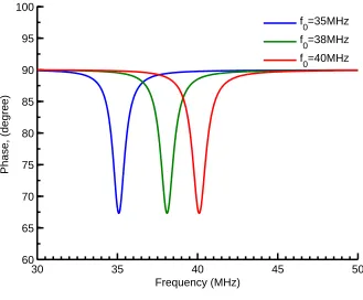
Reader coil inductance,LP 1µH Coupling coefficient,k 0.1 Implant circuit resonant frequency,f0 35, 38, 40M H z

Sensor coil quality factor,Qs 40

tion(3.15)[2]

∆φ∼=arctank2Qs

(3.15a)

∆φ∼₌_arctan2πM2

f0RsLr

(3.15b)

It is preferable to measure the phase of input impedance instead of the magnitude

because of measurable change in the phase in the sensor circuit resonance regime. This can

be seen in Figure 3.4 and Figure 3.5. The circuit parameters that were used to calculate the

phase and amplitude of reader coil impedance are shown in Table 3.1.

Coupling coefficient ”k" is the key factor in limiting the wireless range of inductive

telemetry sensor system. As it can seen from Eq.(3.15), the change in the phase angle (∆φ)

is proportional to square of the coupling coefficient (k) which itself is a function of mutual

inducatance and self inductances of sensor and reader coils. When the reader and sensor

coil axes are aligned, k can be approximated by equation(3.16)[3, 4].

k(z)∼= r

2

srr2

p

rsrr[ p

d2+_r2

r]3

(3.16)

By measuring the phase of the input impedance, one can see a drop in the phase angle

when operating frequency equals the sensor resonant frequency. Fonseca[1]calculated the

(45)

30 35 40 45 50 60

65 70 75 80 85 90 95 100

Frequency (MHz)

Phase, (degree)

f

0=35MHz

f

0=38MHz

f₀=40MHz

Figure 3.4: Reader coil phase

becomes the lowest to the resonant frequency of the implant circuit as

fm i n= f0

1+k

2

4 + 1 8Q2

(3.17)

W he r e, Q= ω0Ls

Rs

(3.18)

Q can also be defined as[5]

Q=2π m a x i m u m e n e r g y s t or e d

t ot a l e n e r g y l os t p e r p e r iod (3.19)

(46)

30 35 40 45 50 160

180 200 220 240 260 280 300 320 340

Frequency (MHz)

Magnitude,(

Ω

)

f

0=35MHz

f

0=38MHz

f₀=40MHz

Figure 3.5: Reader coil amplitude

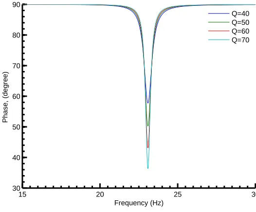
Table 3.2: Design Parameters

Reader coil inductance,LP 2.5µH Coupling coefficient,k 0.12 Implant circuit resonant frequency,f0 23M H z

implant inductor coil has high inductance and low series resistance. Figure 3.6 illustrates the

effect of Q on the phase of reader circuit impedance. The design parameters needed for the

calculation of the impedance are shown in Table 3.2.

Slight misalignment in the axes changes mutual inductance between the coils. As the

distance between coils increases, the coupling coefficient decreases which in turn lowers

the phase dip. This makes it difficult to identify the resonance frequency of sensor circuit

(47)

15 20 25 30 30

40 50 60 70 80 90

Phase, (degree)

Frequency (Hz)

Q=40 Q=50 Q=60 Q=70

Figure 3.6: Effect of Q factor on impedance phase dip

coupling. This problem becomes more acute in the design of intraocular pressure (IOP)

sensor because of the movement of the eyeball relative to the external coil. In order to design

a robust passive telemetry system, the designer needs to identify tolerable limits of coupling

coefficient so that the sensor data can be accurately measured even when the reader and

sensor coil axes are slightly misaligned.

3.2 Surface micromachined MEMS sensor fabrication

Capacitive pressure sensor is well suited to measure intraocular pressure compared to other

kind of pressure sensors such as Piezo-resistive pressure sensors. This is because capacitive

sensors exhibit monotonic response under increased applied pressure[6]. Polysilicon was

selected to be used as structural material for the sensor diaphragm because of low stress

(<1MPa) compared to other materials[7]. The low stress in the films avoids sensitivity

(48)

Figure 3.7: Finite element model of MEMS pressure sensor[9]

A capacitive pressure sensor was fabricated by utilizing a commercially available three

layer polysilicon surface micromachining process called POLYMUMPS[8]. Making use

of commercial MEMS fabrication process cuts down sensor unit cost and also provides

reproducibility because of well studied process parameters. In this process, Polysilicon is

used as the structural material, oxide layer (PSG) is used as the sacrificial layer, and silicon

nitride is used as electrical isolation between the polysilicon and the substrate. Non-planar

surface micromachined pressure sensor has reference pressure cavity above the silicon

wafer surface. The reference cavity is formed by etching away the sacrificial oxide. Since

the IOP range is very small (10 mmHg to 50 mmHg above atmospheric pressure), surface

micromachining fabrication process was deemed to be more suitable compared to bulk

micromachining process. Surface micromachining based sensor fabrication does not require

additional fabrication steps such as wafer bonding, chemical mechanical polishing (CMP).

Surface micromachined sensor also has small form factor compared to bulk micromachined

sensor.

Using the fabrication process data, a finite element model of the MEMS pressure sensor

was developed to calculate the maximum deflection of the movable plate. A plane strain

model of the capacitive pressure sensor is shown in Figure 3.7. On the top surface of sensor,

(49)

(50)

Table 3.3: Movable electrode plate deflection

Plate size,µ×µ Maximum Defleciton,µm

100µm×100µ 0.07

140µm×140µm 0.20 180µm×180µm 0.54

in a capacitive sensor of plate size 100µm×100µm is shown in Figure 3.8. The deflections

of cap sensors of different sizes were calculated from finite element analysis (Table 3.3). As

expected, 100µm×100µm cap sensor is stiffest among the three.

A wide variety of capacitive pressure sensors were fabricated by following a three layer

Polysilicon surface micromachining process. This process has the general features of a

standard surface micromachining process: (1) polysilicon is used as the structural material,

(2) deposited oxide (PSG) is used as the sacrificial layer, and silicon nitride is used as electrical

isolation between the polysilicon and the substrate.

The process begins with 150 mm n−type (100) silicon wafers of 1−2Ω−cm resistivity. The surface of the wafers are first heavily doped with phosphorus in a standard diffusion furnace

using a phosphosilicate glass (PSG) sacrificial layer as the dopant source. This helps to reduce

or prevent charge feedthrough to the substrate from electrostatic devices on the surface.

Next, after removal of the PSG film, a 600 nm low-stress LPCVD (low pressure chemical vapor

deposition) silicon nitride layer is deposited on the wafers as an electrical isolation layer.

This is followed directly by the deposition of a 500 nm LPCVD polysilicon filmPoly0.

Poly0 is then patterned by photolithography, a process that includes the coating of

the wafers with photoresist, exposure of the photoresist with the appropriate mask and

developing the exposed photoresist to create the desired etch mask for subsequent pattern

transfer into the underlying layer (Figure 3.9.1).

(51)

3.9.1 3.9.2

3.9.3 3.9.4

3.9.5 3.9.6

3.9.7 3.9.8

3.9.9 3.9.10

(52)

Figure 3.10: MEMS capacitive sensor after the removal of sacrificial oxide

(Figure 3.9.2). A 2.0µm phosphosilicate glass (PSG) sacrificial layer is then deposited by

LPCVD (Figure 3.9.3) and annealed @1050◦_{C for 1 hour in argon. This layer of PSG, known}

as First Oxide, is removed at the end of the process to free the first mechanical layer of

polysilicon. The sacrificial layer is lithographically patterned with the DIMPLES mask and

the dimples are transferred into the sacrificial PSG layer in an RIE (Reactive Ion Etch) system,

as shown in Figure 3.9.4. The nominal depth of the dimples is 750 nm. The wafers are then

patterned with the third mask layer, ANCHOR1, and reactive ion etched (Figure 3.9.5). This

step provides anchor holes that will be filled by the Poly 1 layer. After etching ANCHOR1, the

first structural layer of polysilicon (Poly 1) is deposited at a thickness of 2.0µm. A thin (200

nm) layer of PSG is deposited over the polysilicon and the wafer is annealed at 1050◦_{C for 1}

hour (Figure 3.9.6). The anneal dopes the polysilicon with phosphorus from the PSG layers

both above and below it. The anneal also serves to significantly reduce the net stress in the

Poly 1 layer.

The polysilicon (and its PSG masking layer) is lithographically patterned using a mask

designed to form the first structural layer POLY1. The PSG layer is etched to produce a

hard mask for the subsequent polysilicon etch. The hard mask is more resistant to the

polysilicon etch chemistry than the photoresist and ensures better transfer of the pattern

into the polysilicon. After etching the polysilicon (Figure 3.9.7), the photoresist is stripped

(53)

After Poly 1 is etched, a second sacrificial PSG layer (Second Oxide, 750nm thick) is

de-posited and annealed (Figure 3.9.10). The Second Oxide is patterned using two different etch

masks with different objectives. ThePO LY1PO LY2V I Alevel provides for etch holes in the

Second Oxide down to the Poly 1 layer. This provides a mechanical and electrical

connec-tion between the Poly 1 and Poly 2 layers. ThePO LY1PO LY2V I A layer is lithographically

patterned and etched by RIE (Figure 3.9.9). The ANCHOR2 level is provided to etch both the

First and Second Oxide layers in one step, thereby eliminating any misalignment between

separately etched holes. More importantly, the ANCHOR2 etch eliminates the need to make

a cut in First Oxide unrelated to anchoring a Poly 1 structure, which needlessly exposes the

substrate to subsequent processing that can damage either Poly 0 or Nitride. The ANCHOR2

layer is lithographically patterned and etched by RIE in the same way asPO LY1PO LY2V I A.

The second structural layer, Poly 2, is then deposited (1.5µm thick) followed by the

deposition of 200 nm PSG. As with Poly 1, the thin PSG layer acts as both an etch mask

and dopant source for Poly 2. The wafer is annealed for one hour at 1050◦_{C to dope the}

polysilicon and reduce the residual film stress. The Poly 2 layer is lithographically patterned

with the seventh mask (POLY2). The PSG and polysilicon layers are etched by plasma and RIE

processes, similar to those used for Poly 1. The photoresist then is stripped and the masking

oxide is removed (Figure 3.9.10).

3.2.1 Sensor Release

The final deposited layer in the PolyMUMPs process is a 0.5µm metal layer that provides

for bonding, electrical routing. The wafer is patterned lithographically with the eighth mask

(METAL) and the metal is deposited and patterned using lift-off. The final, unreleased

Design and Optimization of Passive Wireless Intraocular Pressure Sensor.

ABSTRACT

DEDICATION

BIOGRAPHY

ACKNOWLEDGEMENTS

TABLE OF CONTENTS

LIST OF TABLES

LIST OF FIGURES

ONE

GLAUCOMA

1.1 Glaucoma

1.2 Standard Techniques for IOP Measurement

1.2.1 Applanation (Goldmann) Tonometry

1.2.2 Non-contact Tonometry (Pneumotonometry)

1.3 Need for Continuous IOP Measurement

1.4 Continuous IOP Measurement

1.4.1 Inductively Coupled Telemetry

Passive Devices

Other IOP Measurement Techniques

1.5 Thesis Outline

REFERENCES

TWO

IOP SENSOR DESIGN SPECIFICATIONS

2.1 Implant Location

THREE

SINGLE COIL SENSOR DESIGN

3.1 Single Coil Passive IOP Sensor

3.2 Surface micromachined MEMS sensor fabrication

3.2.1 Sensor Release