Abstract
Mattos, Leonardo Serra. The EvBot II: An Enhanced Evolutionary Robotics Platform Equipped with Integrated Sensing for Control. (Under the direction of Edward Grant.)
The research presented in this thesis describes the design and development of the EvBot II, a small, computationally powerful, and robust evolutionary robotics
platform equipped with an acoustic array system. The EvBot II represents the next generation of autonomous robots for distributed robot-colony research, and its design
has expanded the sensing capabilities and the overall performance of the EvBot robots by the incorporation of two microcontroller units, shaft encoders and a complete acoustic array system for tracking and navigation purposes. The design,
development and test of this new robot is described in detail throughout this thesis, including the design of an USB data acquisition system capable of simultaneously
sampling eight audio channels as required for the realization of the added acoustic array system. Experiments designed to evaluate the performance of this new robot and its components are also described in this thesis, as well as experimental results
T
HEE
VB
OTII
A
NE
NHANCEDE
VOLUTIONARYR
OBOTICSP
LATFORME
QUIPPED WITHI
NTEGRATEDS
ENSING FORC
ONTROLby
L
EONARDOS
ERRAM
ATTOSA thesis submitted to the Graduate Faculty of the North Carolina State University
in partial fulfillment of the requirements for the Degree of
Master of Science
E
LECTRICAL ANDC
OMPUTERE
NGINEERINGRaleigh
April 2003
Biography
Leonardo Serra de Mattos was born December 17, 1974 in Red Bank, New Jersey, and shortly after moved to Brazil with his family. From education received
there he earned his Technical degree in Electronics from the State University of Campinas (UNICAMP) in 1992, and a Bachelor of Science degree in Electrical
Engineering from the University of São Paulo (USP) in 1998. Once again living in the United States, he received his Master of Science degree in Electrical Engineering from the North Carolina State University in 2003. Leonardo is a member of the IEEE
Acknowledgments
I wish to thank my wife Daniela and my parents José Carlos and Theresinha for their love, long support and patience. Together with my brothers and sisters and the rest of my family, they are the ones that give me the strength to grow and always
try to do my best.
I also would like to thank my advisor, Dr. Edward Grant, for accepting me
into the Center for Robotics and Intelligent Machines and for his confidence, enthusiasm and provided assistance. His guidance and friendship are much appreciated. I am also grateful to Dr. John Muth for his assistance, and to my other
committee members, Dr. Troy Nagle and Dr. Mark White for their support and patience.
I also wish to express my gratefulness to Andrew Nelson and Greg Barlow for their help with almost everything related to the EvBots, Kyle Luthy and Chris Braly for their help with acoustic arrays, and all of the members of the CRIM for their
Table of Contents
List of Figures...vi
List of Tables ...ix
List of Abbreviations...x
Chapter 1 – Introduction ...1
Section 1.1 – Thesis Outline ... 3
Section 1.2 – Thesis Goals ... 4
Chapter 2 – Literature Review ...5
Chapter 3 – The EvBot II Platform...10
Section 3.1 – The EvBot II Base ... 11
Section 3.2 - The Encoder Circuitry ... 13
Section 3.3 - The Motor Driver Circuitry ... 16
Section 3.4 – Design of the Utility Printed Circuit Board ... 18
Section 3.6 - The PC/104 Stack ... 22
Section 3.7 – Calibration of the Motion System ... 23
Chapter 4 – Acoustic Array Sensor ...24
Section 4.1 – Quick Background ... 25
Section 4.1.1 – Background on Sound... 25
Section 4.1.2 – Background on Beamforming... 27
Section 4.1.3 – Background on Triangulation ... 28
Section 4.1.3.1 – Triangulation by Solving Simultaneous Equations ... 29
Section 4.1.3.2 – Triangulation by the Voting Method... 31
Section 4.2 – Acoustic Array Software ... 33
Section 4.2.1 – Creating a Representation of the Array Geometry... 34
Section 4.2.2 – Simulating the Directional Sound Intensity Sensed by an Acoustic Array ... 36
Section 4.2.3 – Simulating Beamforming ... 38
Section 4.2.4 – Passive Sonar Simulation and Waterfall Plot... 40
Section 4.2.5 – Simulating Triangulation – Error Plots... 41
Section 4.2.6 – Testing the EvBot’s Tracking Sonar... 44
Section 4.3 – The EvBot’s Acoustic Array Configuration ... 46
Chapter 5 – The USB-DAQ8 Data Acquisition System ...48
Section 5.1 – Commercially Available Data Acquisition Systems ... 50
Section 5.2 – USB-DAQ8 Overview ... 52
Section 5.3 – USB-DAQ8’s Amplifier Circuit ... 54
Section 5.4 – USB-DAQ8’s Low-Pass Filter... 56
Section 5.5 – USB-DAQ8’s Analog-to-digital Converter... 59
Section 5.6 – USB Interface and Controller ... 61
Section 5.7 – The USB-DAQ8’s Timing and Control Circuit... 62
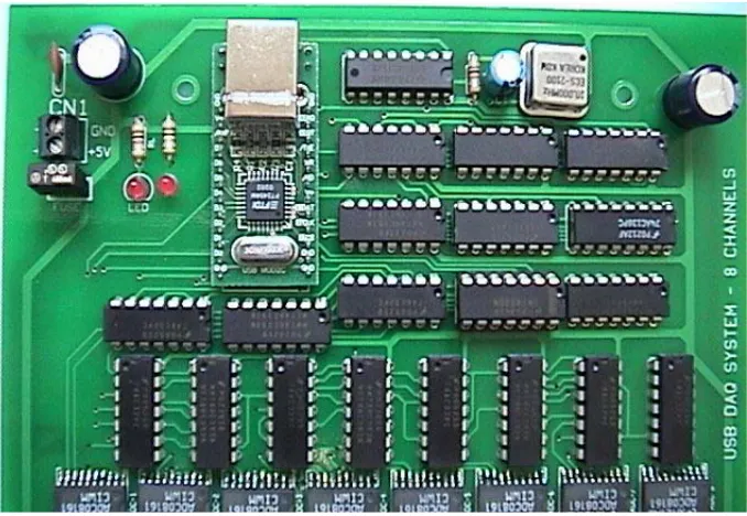
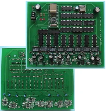
Section 5.8 – USB-DAQ8’s Circuit Board... 66
Section 5.9 – Design Fault and Solution ... 68
Chapter 6 – Experimentation and Results...70
Section 6.1 – Experiments with the EvBot II Platform ... 70
Section 6.1.1 – Calibration of the Open Loop Speed Control ... 71
Section 6.1.2 – Calibration of the Closed Loop Speed Control... 74
Section 6.2 – Experiments with the Data Acquisition System ... 80
Section 6.2.1 – Test of the Low Pass Filter Frequency Response ... 80
Section 6.2.2 – Test of the ADC Linearity and Frequency Distortion... 81
Section 6.2.3 – Test of the Data Transfer Speed... 84
Section 6.2.4 – Acquiring Data with the USB-DAQ8... 88
Section 6.3 – Experiments with the Acoustic Array... 92
Section 6.3.1 – Beamforming by Different Array Configurations ... 92
Section 6.3.2 – Evaluation of the EvBot’s Acoustic Array System... 96
Section 6.3.3 –Using the Acoustic Array as a Tracking Sonar ... 98
Section 6.4 – EvBot’s Navigation by Sound ... 101
Chapter 7 – Conclusion and Future Research ...102
Section 7.1 – Concluding Remarks ... 102
Section 7.2 – Future Research... 104
References ...105
Appendix 1 – Experimental Data ...110
Section A1.1 – Calibration of the Open Loop Control System ... 110
Section A1.2 – EvBot II Speed Control Experiments ... 112
Section A1.3 – Low-Pass Filter Characterization ... 120
Section A1.4 – ADC Linearity and Frequency Distortion... 120
Section A1.5 – USB-DAQ8 Data Transfer Rate Test ... 122
Appendix 2 – Commands for the BasicX MCU’s...124
Appendix 3 – Datasheets ...134
A3.1 – MZ104 computer... 135
A3.2 – DiskOnChip 2000... 136
A3.3 – PCM-3115B PCMCIA Module... 138
A3.4 – PCMCIA Wireless Card ... 139
A3.5 – BasicX24 Microcontroller ... 141
A3.6 – ENS-1J-B28 Rotary Optical Encoder... 142
A3.7 – HCTL-2016 Quadrature Decoder... 144
A3.8 – HS-300BB Servo Motor ... 146
A3.9 – L298 Dual Full-Bridge Driver... 148
A3.10 – UC3610 Dual Schottky Diode Bridge... 150
A3.11 – 74HC165 Parallel-in / Serial-out Shift Register... 152
A3.12 – MIC29501 Voltage Regulator... 154
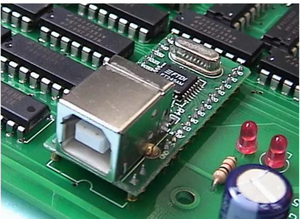
A3.13 – USB MOD2 ... 156
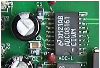
A3.14 – ADC8161 Analog to Digital Converter ... 158
A3.15 – LMX324 Quad Operational Amplifiers ... 160
A3.16 – LTC 1563-3 Active Lowpass Filter ... 162
A3.17 – WM-52B Omnidirectional Electret Microphone ... 164
A3.18 – 74VHC112 J-K Flip-Flop ... 165
A3.19 – 74AC74 D-Type Flip-Flop ... 167
A3.20 – 74VHC393 Dual 4-Bit Binary Counter... 169
A3.21 – 74AC32 Quad 2-Input OR Gate... 171
A3.22 – 74AC138 1-of-8 Decoder ... 173
A3.23 – 74HC30 8-input NAND Gate... 175
List of Figures
Figure 3.1: The Bedlam, used as the EvBot II base... 11
Figure 3.2: Encoders installed on the EvBot II base using a custom designed bracket. ... 12
Figure 3.3: Motor-Encoder Assemblage... 13
Figure 3.4: Encoder circuitry in the utility board. ... 15
Figure 3.5: Motor driver circuit in the utility board... 17
Figure 3.6: Top layer of the utility board... 19
Figure 3.7: Bottom layer of the utility board. ... 19
Figure 3.8: The manufactured utility board. ... 20
Figure 3.9: The EvBot II completely assembled, showing the utility board and the PC/104 stack mounted on the top the threaded base... 22
Figure 4.1: Sound waves in air (reproduced from [38]). ... 26
Figure 4.2: Constructive and destructive interference (reproduced from [38]). ... 27
Figure 4.3: Setup for formulation of the triangulation problem (reproduced from [18])... 29
Figure 4.4: Setup for formulation of the triangulation problem. ... 31
Figure 4.5: (A) MATLAB running the program CreateAcArray.m and (B) created array. ... 35
Figure 4.6: Example of simulated acoustic signals. (A) Signal at the sound source. (B) Delayed signals arriving at the microphones. (C) Resulting signal showing destructive interference cause by linear combination of the sensors’ signals. ... 37
Figure 4.7: Example of directional gain plots generated by the ArrayPolarPlot program. ... 38
Figure 4.8: Simulated image of a beam that was formed for a look-angle of 45° azimuth and 0° elevation... 39
Figure 4.9: Graphics generated by the program TrackingSonar... 41
Figure 4.10: Simulated Error plots from the use of the EvBot’s acoustic array to estimate the direction of a sound source. (A) Matrix method. (B) Voting method. ... 43
Figure 4.11: Directional sound magnitude as viewed by the EvBot. The green line marks the azimuth of maximum magnitude. The plot’s title displays the generated movement command. ... 45
Figure 4.12: Graphics generated by the program EvBot_TrackingSonar when a helicopter’s sound was being reproduced near the robot... 45
Figure 4.13: Acoustic array configuration for the EvBot II... 46
Figure 4.14: Simulation of the directional sound magnitude sensed by the EvBot’s acoustic array due to a 1 KHz sound source at azimuth 45°... 47
Figure 4.15: The EvBot II equipped with its acoustic array and data acquisition board. ... 47
Figure 5.1: The USB-DAQ8 block diagram. ... 53
Figure 5.3: Waveforms at the input (Ch 1) and output (Ch 2) of the amplifier circuit.
... 56
Figure 5.4: Gain and phase frequency response of the USB-DAQ8’s active filter. ... 58
Figure 5.5: A single low-pass filter seen on a section of the USB-DAQ8 printed circuit board. ... 58
Figure 5.6: Analog-to-digital converter on a section of the USB-DAQ8 board... 60
Figure 5.7: The USBMOD2... 61
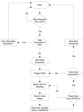
Figure 5.8: USB-DAQ8’s functional block diagram ... 64
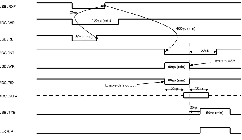
Figure 5.9: Timing diagram for the USB-DAQ8 data acquisition system. ... 65
Figure 5.10: Logic circuit for timing and control on the USB-DAQ8 board. ... 66
Figure 5.11: CirCAD drawing of the USB-DAQ8’s top layer. ... 67
Figure 5.12: CirCAD drawing of the USB-DAQ8’s bottom layer. ... 67
Figure 5.13: The USB-DAQ8’s printed circuit board. ... 68
Figure 6.1: Open loop calibration points for linear motion. Error bars show ±5% error at each calibrated speed. ... 72
Figure 6.2: Open loop calibration points for clockwise rotations. The y axis represents the product of PMW values and active time of the rotation commands. The error bars show ±5% error at each calibrated point... 73
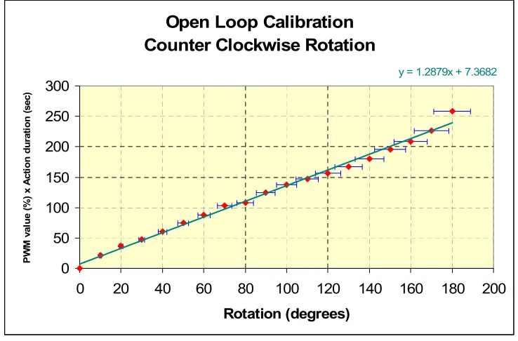
Figure 6.3: Open loop calibration points for counter clockwise rotations. The y axis represents the product of PMW values and active time of the rotation commands. The error bars show ±5% error at each calibrated point... 73
Figure 6.4: Distance traveled by the EvBot II for different speed commands when using closed-loop speed control... 75
Figure 6.5: Response of the speed control system to different commanded speeds obtained from experimental data. ... 76
Figure 6.6: EvBot II traveling through the maze in search of the red goal (two trials). ... 78
Figure 6.7: Two generations of EvBots playing together... 79
Figure 6.8: Simulated world with simulated EvBots running the same neural network controllers as the one used by the real robots (courtesy of Andrew Nelson, CRIM)... 79
Figure 6.9: Frequency response USB-DAQ8’s low-pass filter. ... 81
Figure 6.10: Results from the linearity test performed on the IC ADC08161C. ... 82
Figure 6.11: Results from the linearity test performed on the IC ADC08161C. The expected error reflects the ±0.02V resolution (5V / 256 levels)... 82
Figure 6.12: Results from the frequency distortion test performed on the IC ADC08161C and data acquisition system. ... 83
Figure 6.13: Errors measured during the frequency distortion test performed on the IC ADC08161C and data acquisition system. ... 84
Figure 6.14: Total number of bytes transferred as a function of sampling time... 86
Figure 6.15: Transfer rate in bytes per second as a function of the sampling time. ... 86
Figure 6.19: USB-DAQ8 acquiring a 4.53 KHz signal. ... 90 Figure 6.20: The program USBscope displaying data simultaneously sampled from all eight input channels of the USB-DAQ8. ... 91 Figure 6.21: Beamforming simulation for a frequency of 1 KHz using a planar array
that would fit on the top of the PC/104 stack... 93 Figure 6.22: Beamforming simulation for a frequency of 1 KHz using a 3-D array
configuration that could fit on the EvBot II body... 94 Figure 6.23: Beamforming simulation for a frequency of 1 KHz using the final array
configuration selected for the EvBot II... 95 Figure 6.24: Comparisons between beam patterns obtained from real data (right) and
simulated data (left) for the following sound frequencies: (A) 200 Hz. (B) 500 Hz. (C) 1000 Hz... 97 Figure 6.25: Comparisons between beam patterns obtained from real data (right) and
simulated data (left) for the following sound frequencies: (A) 1200 Hz. (B) 1500 Hz... 98 Figure 6.26: Acoustic array system being used to track the sound of truck reproduced
by a nearby moving speaker. ... 99 Figure 6.27: Acoustic array system being used to track a single-tone sound source.100 Figure 6.28: Path taken by the EvBot II to find the sound source... 101 Figure A1.1: Measured distance traveled versus time for a commanded speed of one
inch/second. ... 114 Figure A1.2: Plot of velocity versus time for a commanded speed of one inch/second.
... 114 Figure A1.3: Measured distance traveled versus time for a commanded speed of two
inches/second. ... 115 Figure A1.4: Plot of velocity versus time for a commanded speed of two
inches/second. ... 115 Figure A1.5: Measured distance traveled versus time for a commanded speed of three
inches/second. ... 116 Figure A1.6: Plot of velocity versus time for a commanded speed of three
inches/second. ... 116 Figure A1.7: Measured distance traveled versus time for a commanded speed of four
inches/second. ... 117 Figure A1.8: Plot of velocity versus time for a commanded speed of four
inches/second. ... 117 Figure A1.9: Measured distance traveled versus time for a commanded speed of five
inches/second. ... 118 Figure A1.10: Plot of velocity versus time for a commanded speed of five
inches/second. ... 118 Figure A1.11: Measured distance traveled versus time for a commanded speed of six
inches/second. ... 119 Figure A1.12: Plot of velocity versus time for a commanded speed of six
List of Tables
Table 3.1: Control signals for the motor driver L298... 17
Table A1.1: Calibration values obtained for linear motion. ... 110
Table A1.2: Calibration values obtained for rotations... 111
Table A1.3: Measured speed versus time for different commanded speeds... 112
Table A1.4: Measured distance traveled versus time for different commanded speeds ... 113
Table A1.5: Measured values for gain and phase as a function of frequency. ... 120
Table A1.6: Values obtained during the linearity test performed on the IC ADC08161C. ... 121
Table A1.7: Values obtained during the frequency distortion test performed on the IC ADC08161C. ... 122
Table A1.8: Results from data transfer tests performed while using a sampling frequency of 78.125 KHz. The values in the table represent and average of 100 trials performed for each acquisition time. ... 123
List of Abbreviations
ADC = Analog to Digital Converter AI = Artificial Intelligence
ATA = Advanced Technology bus Attachment
CRIM = Center for Robotics and Intelligent Machines DIP = Dual Inline Package
DOC = DiskOnChip
GPS = Global Positioning System GUI = Graphical User Interface I/O = Input/Output
IEEE = Institute of Electrical and Electronics Engineers MCU = Microprocessor Control Unit / microcontroller NCSU = North Carolina State University / NC State PCB = Printed Circuit Board
PCMCIA = Personal Computer Memory Card International Association PnP = Plug-and-Play
PWM = Pulse Width Modulation RF = Radio Frequency
RSTA = Reconnaissance, Surveillance and Target Acquisition SAR = Search and Rescue
SDRAM = Synchronous Dynamic Random Access Memory SONAR = Sound Navigation and Ranging
Chapter 1 – Introduction
Researchers in the areas of distributed and evolvable robotics have recently started to use physical platforms to validate concepts developed in simulation, but one
of the problems that they have been facing is to overcome limitations imposed by unsuited robotic systems. We believe that the current need in this area is for robot
platforms that are small enough to be used within research laboratories, yet robust and computationally power enough to implement complex machine-learned controllers in the real world. The EvBot robots were developed to bridge the gap that exists
between cumbersome commercial platforms featuring powerful central processing units (CPUs) and extensive sensing capabilities, and small inexpensive robots with
limited capabilities. The original EvBot measures only eight inches in diameter and is an autonomous system equipped with a Pentium class microcomputer system. This robot has proven to be an extremely useful platform for advanced experimentation in
robot colony behaviors and evolutionary robotics, but experimentation also indicated that the original EvBot platform still needed additional sensor capabilities to improve
position and velocity control. The research reported upon in this thesis concentrates on specifying the design of, and the implementation of, an improved and flexible hardware architecture for hosting and integrating data from a variety of sensor types,
robots acting as part of a colony. To support this effort, circuitry was designed to enable the incorporation of shaft encoders and the closed loop control of up to three motors. A USB hub was also introduced to allow uncomplicated incorporation of
extra sensors if and when such sensors are required. The USB hub allows “plug and play” sensor addition, and was used for the integration of an acoustic array system
specially developed for this robot. The development of the mentioned acoustic array system was the second major focus of the research described in this thesis, and it involved the design of a custom data acquisition system (the USB-DAQ8) and several
associated software programs. The EvBot II autonomous robot that emerged from this research work extends the possible application areas of EvBots, e.g., evolutionary and
distributed robotics to undertake surveillance, reconnaissance and security applications. Experimentation with the EvBot II robotic platform demonstrated that, in addition to be completely compatible with the original EvBot, it is able to make
successful use of the shaft encoders to control its traveling speed. Experiments also confirmed that the developed data acquisition system can effectively perform the simultaneous sampling of eight audio channels at a rate of 9600 samples per second
Section 1.1 – Thesis Outline
The design and development of the EvBot II platform and its custom acoustic array system are described in this thesis. Chapter 2 presents a review of the literature,
including a summary of autonomous robots currently in use in the areas of distributed and evolutionary robotics, and an overview of past and current research focused on the use of acoustics by mobile robots. The development of the new hardware and
software for the EvBot II, including the design of the encoder systems and the new circuitry to drive the motor, is presented in Chapter 3. The following chapter presents an introduction to acoustic arrays and describes software developed for simulation
and use on such systems. Chapter 5 provides an in depth description of the data acquisition system USB-DAQ8, which was developed to realize the acoustic array.
The experimental results from tests of the robot platform and acoustic array system are presented in Chapter 6. Lastly, Chapter 7 presents some ideas for further improvements of the EvBot platform, as well as ideas for future experiments with the
Section 1.2 – Thesis Goals
The objectives of this thesis are to describe the:
• Design and construction of the EvBot II, a small but computationally
powerful autonomous robot created as an enhanced version of the original
EvBot.
• Development of the software used to design and make use of the
acoustic array system implemented on the EvBot II.
• Design of the USB-DAQ8, a data acquisition system custom
developed to realize the EvBot’s acoustic array system.
• Demonstration of the robot’s enhanced performance and use of the
Chapter 2 – Literature Review
The concept of robots is a very old one in our society and has always been related to automatic machines that can perform tasks in the manner of a human. Although their history is frequently said to have started around 270 BC with the water
clocks and organs made by the Greek engineer Ctesibus, it was only in the early 1920’s that term “robot” appeared. It was introduced by the Czech writer Karel
Capek, who derived the term from the Czechoslovakian word for slave (robotnik) and used it in the play “Rossum’s Universal Robots”.
From the beginnings, one of the main functions of robots in our society has
been to free humans from repetitive, difficult or harmful tasks. Industrial robots were the first ones to appear in large scale and, since their first demonstration in 1959 by
the M.I.T. Servomechanisms Lab, they have been improving the quality of life of humans across the globe. In recent times mobile robots have also started to be designed to help humans in a diverse quantity of tasks, from household work to
exploration of hazardous environments. However, unlike industrial robots, mobile robots are required to have intelligence, the capability to adapt to different
[4] [8], security monitoring [24] [27] [32] and search and rescue (SAR) in disaster areas [6] [23].
The first autonomous robots appeared in the research community in the early
1950’s when the neurophysiologist W. Grey Walter [29] introduced his “Machina Speculatrix”, which was a three wheeled vehicle equipped with a two vacuum tube
analog computer. This robot had the tendency to wonder around exploring the environment and this was the first proof that intelligent and autonomous robots can evolve and develop practical functions. Though it was only it the late 1980s that
researchers would expand that idea to groups of robots that evolve together, originating in what is now known as distributed robotics [10] [2] [1] [30]. About that
same time the artificial intelligence (A.I.) research community was introduced to the subsumption architecture proposed by Rodney Brooks [3] and started using its essence to build physical platforms to realize and test intelligent systems that
previously had only existed in simulations.
From the early work up to recent days, many of the physical autonomous robots developed to test evolvable and distributed systems were unsophisticated and
carried little onboard processing, such as the common Kephera robot [35], which has been used by innumerous research groups as mentioned in [21]. Even though these
Recently autonomous robots with large processing capabilities have appeared in the distributed robotics literature, such as the Urban II and the ATRV-2 developed by iRobot Corporation and used by Hogg et al. [12] and Budulas et al. [4]. These
robots use powerful hand-held computers for processing of sensor data and control, but are relatively large, heavy and expensive. Another example of a powerful robot is
the RATLER, which is a medium-sized all-electric vehicle containing a PC104 stack for computation, control and sensing. The RATLER was originally developed at the Sandia National Laboratories as a prototype vehicle for lunar missions, and some of
these robots are currently in distributed robotics research [8] [16].
Other research groups are experimenting with evolvable and distributed
systems using small and inexpensive robots, like the GROWBOT from Parallax [39], which was used in the Idaho National Engineering and Environmental Laboratory (INEEL) by a research group working on large-scale micro-robotic forces [7]. Even
with the limited processing power and limited sensorial capabilities provided by GROWBOT’s Basic Stamp 2 microcontroller, the researchers were able to demonstrate evolution and interaction between robots.
The robot EvBot developed in the Center for Robotics and Intelligent Machines (CRIM) at the NC State University [11] fits well into the mid-range of
robots [35], the EvBot uses a PC104 stack equipped with a Pentium class processor, and it also features low power consumption, being able to continuously operate for more than two hours on a single 7.2V/3000mAh Ni-MH battery.
In general, it is seen that the research community in the area of distributed and evolvable robotics requires robotic platforms that allow the implementation of
computationally complex controllers from a wealth of data. This is especially true when the robots are designed to leave the research laboratories and undertake “real-world” tasks. In the “real-“real-world” the usefulness of such robots is usually directly
proportional to the diversity of their onboard sensors, i.e. the larger the variety of sensors one robot has, the higher is the number of possible tasks it can perform, or the
higher is the precision of the tasks it can perform. For that reason, this research area needs robot platforms whose architecture is open and expandable, thus providing a capability for the addition of new sensors as needed. Robots being developed for
military applications, such as urban warfare, are very good examples of systems with these needs [16] [19]. They are usually required to have video camera, radar, GPS, RF transceivers and other specialized sensors, like chemical detectors or acoustic
sensors.
Recently the researchers in the area of robotic RSTA started to revisit the
acoustic field and the use of sound as tactical information has been regaining importance. This field started to become very popular by the end of the World War I, when the first sonar devices were developed to detect submarines. Since them the
acoustic arrays and related technologies, such as systems that perform spatial filtering by beamforming [28], target localization and classification [13] and estimation of sound source location [5] [18]. Acoustic array research is still active and producing
knowledge, especially in the area of sensor array data processing [14] [25].
Recent trends in security and in RSTA are also bringing the attention back to
passive acoustic array systems due to the fact that such systems can provide important strategic information without being easily detected. For that reason, acoustic array systems are being studied as part of RSTA robots [31] and as unattended ground
sensors (UGS) [17].
In conclusion, it is seen that the research in the area of autonomous mobile
robotics is growing substantially and strengthening in the area of distributed robotics. This is particularly the case where a team of robots may contribute cooperatively and overperform an individual robot. As a result, small and sophisticated robot platforms
Chapter 3 – The EvBot II Platform
The original Evolutionary Robots (EvBots) [11] have always performed well,
but they needed more on-board sensors to increase their perception and control. For example, they needed the addition of shaft encoders to ensure closed-loop speed
control. Without encoders it is not possible for the robot to perform precise movements, or move at a constant speed, or realize that it is not moving at all. Without shaft encoders each EvBot has to go through a difficult and time-consuming
calibration process to ensure the robot controller makes precise decisions related to desired actions, e.g., turning a desired amount or moving at a desired speed.
So, the addition of shaft encoders became the first priority in the design of the new EvBot robot platform, the EvBot II. The encoders along with their associated circuitry were the first major design change initiated for expanding the robot colony. Because the EvBot II colony was to be based on the Radio Shack Bedlam product
(see Figure 3.1), a certain amount of redesign was needed to its hardware, e.g., replacement of the driving motors and the removal of the extra gears. Only then
could the new circuit design required for motor control and enhanced sensing be specified. To expand the connectivity of the original EvBot systems, a USB hub was also included on the EvBot II robot platform. Doing this ensured that the new system
The specification and the design of all hardware and software for the new generation of EvBots will be fully described in the remaining sections of this chapter.
Section 3.1 – The EvBot II Base
The base used for the EvBot II came from the radio-controlled car Bedlam, from Radio Shack. Driving the car showed that it operated at high speeds, using its
tank-like traction system for forward and backward motion, and spins. However, this vehicle also includes a third axis that can provide transverse motion, which makes an
interesting platform for studying the use of biologically inspired actions, subsumption architectures, and evolutionary robotics.
Figure 3.1: The Bedlam, used as the EvBot II base.
which were kept as the basis of the EvBot II platform. The shaft encoders were then installed in the base using a custom designed support (Figure 3.2) and the motor wire loom were extended to ensure that they would be able to connect to the newly
designed driver board.
Figure 3.2: Encoders installed on the EvBot II base using a custom designed bracket.
After the changes to the mechanical drive system were made to the Bedlam vehicle, it now became the basis of the EvBot II robot platform. Speed control tests
carried out with the Bedlam drive system showed that the original motors operated too fast for all practical purposes. It therefore became necessary to reduce the speed of the drive system, which the tests showed could not be solely achieved by simply
reducing the motor’s voltage. Because the radio-controlled car was design to move at high speed, the gearing does not provide a sufficient enough reduction to keep the
motor in its operating range, particularly when the robot is required to move slowly. New motors having built-in reduction gears were specified to overcome this problem. The selected motor was the HS-300BB made by Hitec (Appendix A3.8). Once these
they could not be installed without another design alteration being made to the Bedlam body. The final design of the bracket supported the drive motors and the encoders, and is shown in Figure 3.3.
Figure 3.3: Motor-Encoder Assemblage.
Section 3.2 - The Encoder Circuitry
The addition of shaft encoders to each of the robot’s motors required the
development of dedicated hardware and software capable of handling the data from these two sensors. To achieve this, encoder circuitry was specially designed, tested
The encoder circuit is based on the integrated circuit HCTL-2016 from Agilent, see the data sheet in Appendix A3.7. This integrated circuit (IC) is a quadrature decoder/counter set up to be directly controlled by a microcontroller chip,
which in this case is the BasicX24. The data sheet of the HCTL-2016 shows that the chip outputs a 16-bit word to an 8-bit parallel bus. This is achieved by breaking the
16-bit word into two 8-bit bytes, i.e., a high byte and a low byte. The output byte is selected by control lines of the microcontroller, but due to the limited number of I/O pins on the BasicX a parallel to serial converter had to be employed to get the
appropriate data control action. A shift register, IC MM74HC165, was selected for this task. Adopting this design means that only one control line is now required from
the BasicX microcontroller.
The encoders selected for this application are the optical encoder ENS-1J-B28 from Bourn, see Appendix A3.6. This encoder provides a 2-bit gray code as output
and its the maximum shaft speed is 3000 RPM. After the encoders, the only other required component for the new circuitry is a clock oscillator. This needs to be connected to the decoder and it should be fast enough to allow proper functioning of
the system at the maximum desired speed. Given the maximum operating speed of the encoder, the selected clock oscillator was an ECS100AC, which is a 1.22MHz
oscillator from ECS International Inc.
The BasicX microcontroller is equipped with internal timers and circuitry that is capable of driving two simultaneous pulse width modulation (PWM) outputs.
shaft encoders on the EvBot platform. The final circuit design for the shaft encoders, see Figure 3.4, has the two shaft encoder systems working in parallel to ensure maximum operating efficiency.
Figure 3.4: Encoder circuitry in the utility board. Clock
Oscillator
Decoders
Shift Registers
Section 3.3 - The Motor Driver Circuitry
This part of the EvBot II system design deals with the speed control of a DC motor using pulse width modulation (PWM). The PWM signals, which are a train of square waves where the aspect ratio can be altered, are generated in the EvBot II by
the BasicX microcontroller and are used to control the speed of the DC motors. By introducing an H-Bridge driver into the circuit for power amplification, power can be supplied to drive the DC motors and the control of forward/reverse direction of
rotation of the motor is easily implemented.
To make use of the BasicX microcomputer’s capability of producing two
simultaneous PWM outputs, the Dual Full Bridge Driver L298 was selected. This is a compact but powerful IC capable of driving two DC motors with current up to 4A, see Appendix A3.9. Each of the two halves of the L298 driver has an enable pin and
two input pins that can accept the TTL level signals produced by the BasicX. The input pins are used to select the direction of rotation and the enable pin receives the
Table 3.1: Control signals for the motor driver L298.
Input 1 Input 2 Enable A Motor
X X Low Free running
High Low High Turn clockwise
Low High High Turn counter-clockwise Low Low
High High Illegal / Not Possible
To ensure that the signal on the Input 2 pin is always the inverted signal of the Input 1 pin, the inverter IC 7404 was used. DC motor back-EMF protection was also
included in the circuit through the addition of the small signal Schottky diodes encapsulated on the IC UC3610 chip from Texas Instruments, see Appendix A3.10.
Figure 3.5: Motor driver circuit in the utility board. Microcontrollers
Motor Drivers (L298)
Section 3.4 – Design of the Utility Printed Circuit Board
The utility board in the EvBot II integrates several functions. First, it is
responsible for powering the PC/104 stack, which contains the central processing unit (CPU). Second, it is responsible for all interface connections, such as the mouse, keyboard, speaker, reset button and a USB port access to the CPU. Other than these
utility functions, the board design also incorporates two BasicX microcontrollers and all the necessary circuitry for driving the DC motors and interfacing to the shaft
encoders.
The utility board was designed to conform to the geometry of the Bedlam vehicle’s base, to the extent that it uses the pre-existing holes in the vehicle for
attachment. The board has two wiring layers and was drawn using the software CirCAD. Images of the CAD design of top and bottom layers of the utility board are
Figure 3.8: The manufactured utility board.
Section 3.5 –CPU to
M
icrocontroller
C
ommunication
S
ystem
As in the original EvBot design, all communications between the CPU (PC/104-based) and the microcontrollers (BasicX-based) in the EvBot II design are
made using the RS232 communications standard. The main difference between the communications system design between the original and the new systems is that there
of design it was decided to use only one of the serial ports in the CPU for data transfers. To solve this problem a communications chain was developed.
The communications system starts on the serial port 1 of the PC/104 stack.
That port is directly connected to the first BasicX microprocessor, which is called the Master BasicX. The second link is made using the BasicX chip to support and handle
extra serial ports. A second RS232 port is thus defined in the Master BasicX and I/O pins are allocated to communicate serially to the second microcontroller, called the Slave BasicX.
All the commands in this communication system originate in the CPU and are sent to the Master BasicX. This microcontroller is responsible for determining if
received commands should be executed locally or if they should be forwarded to the Slave BasicX for execution. All system commands are one-byte in length, which can be extended to include arguments if necessary (see Appendix 2). All system
Section 3.6 - The PC/104 Stack
The PC/104 stack contains the MZ104, the central processing unity (CPU) of
all EvBot’s. It is based on the integrated circuit ZFx86, a Pentium-class processors whose main features include: 32 bit CPU core with 100 MHz operation; Full desktop AT compatibility; 64 MB of SDRAM; Fail-safe boot ROM; Dual watchdog timer;
Two serial ports; One parallel port; One USB port; Drive interfaces and support for a solid state flash memory device (DiskOnChip).
The second component in the PC/104 stack is a PC/104 interface module with two built-in PCMCIA card slots. It is used to hold additional memory (128 MB in a flash card) and a wireless network card.
A detailed description of the hardware and custom software developed for the PC/104 system for the EvBots’s can be found in [11]. That work also presents the configuration of the network environment were the EvBot’s operate and the Infinity
Atom Linux, the custom operational system developed for the EvBot platform.
The only improvements on the PC/104 system implemented in the EvBot II
were the expansion of memory size. The flash memory card was upgraded from 96MB to 128MB and the DiskOnChip size was increased from 8MB to 32MB. The remainder of the PC/104 system was kept as specified for the original EvBot’s
platform.
Section 3.7 – Calibration of the Motion System
Although the EvBot II incorporates shaft encoders, calibrations of the motion
system were necessary to guarantee a reliable performance of the robot. The calibrations were performed for the open-loop and closed-loop control modes and
Chapter 4 – Acoustic Array Sensor
Acoustic arrays are passive sensor systems that can have several uses with a robot platform [4] [13]. They are composed by a group of acoustic sensors placed in known geometrical locations that can, in connection with a processing unit, perform a
number of audio related functions. Just like our ears, acoustic arrays can be used for communications, for navigation purposes, or as passive sonar for monitoring,
tracking, object identification and triangulation.
One of the advantages of acoustic arrays is that they offer increased acoustical sensitivity when compared to single sensor systems, but the main reason to use such
an array of sensors is the possibility to perform beamforming and triangulation with the acquired audio data. Both of these functions are based on phase differences
between the multiple audio signals. Beamforming provides a way to implement spatial filtering and directional listening, while triangulation can be used to pinpoint the coordinates of a sound source with respect to the sensors array. Both functions
will be detailed later in this chapter.
Acoustic arrays started to gain importance when the first sonar devices were
developed by the end of the World War I. Since then they have been widely used in the field of surveillance and target acquisition. Recently the use of acoustic arrays started to be extended to autonomous mobile robots being designed for applications in
usefulness for target detection and situation awareness, such as location of snipers or detection of door slam [31].
The goal of the development of an acoustic array for the EvBot II is to expand
its sensorial capabilities and to enable the investigation of the uses of sound as another source of information about the robot’s surrounding world. With this
objective, a small area acoustic array with eight microphones was designed in simulation and later implemented as a shield that can be attached to the robot body.
This chapter briefly presents the background theory involved in acoustic array
systems, and presents simulation programs developed to help the understanding and design of such arrays. The programs include software to analyze acoustic array
configurations for beamforming and triangulation purposes, and programs developed to use and analyze real acoustic arrays. As a group the developed programs provide the means to validate simulation data and to demonstrate the usefulness of an acoustic
array system to the EvBot II.
Section 4.1 – Quick Background
Section 4.1.1 – Background on Sound
Sound propagates through air as a longitudinal wave, which is characterized by the medium being displaced in parallel to the propagation of the wave. As an example, “a single-frequency sound wave traveling through air will cause a sinusoidal
pressure variation in the air. The air motion which accompanies the passage of the sound wave will be back and forth in the direction of the propagation of the sound”
[38].
Figure 4.1: Sound waves in air (reproduced from [38]).
The propagation speed of sound is determined by the properties of the
medium and, as most other types of waves, follows the relationship v = f λ, where v is
the propagation velocity, f is the wave frequency and λ is the wavelength. In the case
of dry air, the speed of sound can be approximated by vsound ≈331.4+0.6T m/s, where T is the Celsius temperature. As an example, for dry air at 21°C the sound
speed is 344 m/s and the audible sound waves have wavelengths from 0.0172 meters
Section 4.1.2 – Background on Beamforming
Beamforming is a method used to implement spatial filtering of signals in an
array of sensors. It is realized by beamformer systems that collect spatially propagating waves and exploit the principle of interference in order to receive a signal radiating from a specific location and attenuate signals from other locations.
Interference is a phenomenon that can occur between waves propagating in the same medium, and may be constructive or destructive. Constructive interference
occurs when the interfering waves are “in phase” and their amplitudes add. If the waves are “out of phase” and the amplitudes subtract the interference is called destructive.
Figure 4.2: Constructive and destructive interference (reproduced from [38]).
signals coming from other directions to interference destructively. This effectively amplifies the signals coming from the listening direction and attenuates signals from other directions.
Typically a beamformer is a digital processing system that contains a data acquisition system to translate the analog input data into digital information by means
of a sampling process. In such a beamformer the sampled time series obtained from each sensor is shifted and linearly combined to generate a single output time series, which is taken as the signal coming from the specific listening direction.
Section 4.1.3 – Background on Triangulation
Triangulation is a term used to indicate the calculation of the coordinates of a
signal source based on multiple sensors’ data (or the coordinates of the receiver based on multiple sources’ signals). In the case of acoustic arrays, the coordinates of the sound source can be calculated based on the coordinates of each sensor in the array
and on the time delays between the signals received by each sensor. Different algorithms can be used to perform such calculation, and they usually provide different
Section 4.1.3.1 – Triangulation by Solving Simultaneous Equations
The triangulation method described in this section was called “Matrix Method” and its formulation is relatively simple. As described in [18], the solution
can be developed from the case where there is one signal transmitter and four receivers (sensors):
Figure 4.3: Setup for formulation of the triangulation problem (reproduced from [18]).
To start the formulation, consider that the position of the sound source (u,v) is
unknown, but the coordinates of the sensors are known and have the values R1 (x1,y1),
R2 (x2,y2), R3 (x3,y3) and R4 (x4,y4). Also consider that we can measure time delays
between the received signals and assume sensor number 1 as the reference. So the time delays are given by ∆T12, ∆T13 and ∆T14. Now, considering that the sound
+ c∆T13) and (d + c∆T14), where c is the speed of the sound. At this point we already
have a set of equation, which is: (x1 – u)2 + (y1 – v)2 = d2
(x2 – u)2 + (y2 – v)2 = (d + c∆T12)2
(x3 – u)2 + (y3 – v)2 = (d + c∆T13)2
(x4 – u)2 + (y4 – v)2 = (d + c∆T14)2
Now, by solving the first equation for d2 and performing some substitutions, the final set of equations can be written:
− − + + ∆ − − + + ∆ − − + + ∆ = ∗ ∆ − − − ∆ − − − ∆ − − − 2 4 2 4 2 1 2 1 2 12 2 2 3 2 3 2 1 2 1 2 13 2 2 2 2 2 2 1 2 1 2 12 2 14 4 1 4 1 13 3 1 3 1 12 2 1 2 1 2 2 2 2 2 2 2 2 2 2 2 2 2 2 2 y x y x T c y x y x T c y x y x T c d v u T c y y x x T c y y x x T c y y x x
These simultaneous equations can be solved for the sound source coordinates
(u,v) and for the distance d between the transmitter and the sensor number 1 provided that we know the velocity of the sound. If that velocity also needs to be calculated, the addition of a fifth sensor can provide an extra equation and a new set of equations
can be found and solved. This formulation can also be extended to three-dimensional arrangements (see [18] for details).
This algorithm was tested in simulation and it was found that it is sensitive to errors in the sensors coordinates and in the time delays measurements. It also presents many singular points for planar arrays, so a new algorithm was developed to try to
Section 4.1.3.2 – Triangulation by the Voting Method
This algorithm was developed to approximately determine the azimuth angle of an emitting sound source and can be applied to arrays of arbitrary number of
sensors and arbitrary configurations. The formulation of the triangulation problem for this method can be better understood by analyzing an acoustic array composed of 3 microphones positioned on the same plane:
Figure 4.4: Setup for formulation of the triangulation problem.
For the development of the equations, consider the reference microphone to be the mic 1, the microphone with the smallest measured time delay. Now, remembering
d3,1m d3m d2,1 d2,m θss,3 θ3,1 mic 1
(x1,y1)
t1
α
β
mic 3 (x3,y3)
t3 mic 2 (x2,y2)
t2
Y
X
d3,1= distance between mic 3 and
reference mic
θ3,1= azimuth of the vector from mic 3 to
reference mic
d3,m= calculated distance based on time
delay between mic 3 and reference mic.
θss,3= bearing of the sound source from
d3,1), as well as the azimuth of the vectors from each microphone to the reference (θ3,1
and θ2,1), relative time delay measurements can be used to calculate the distances d2,m
and d3,m. The formula for these calculations are based on the speed of the sound and
given by:
) ( 2 1
,
2 V t t
d m = sound ∗ −
) ( 3 1
,
3 V t t
d m = sound∗ −
If we consider that the acoustic array is in the far field of the sound source, square angles can be assumed as shown in Figure 4.4, and using geometrical relations we can
get to the following equations:
2 1 3 2 1 3 1 ,
3 (x x ) (y y )
d = − + − 2
1 2 2 1 2 1 ,
2 (x x ) (y y )
d = − + −
= − 1 , 3 , 3 1 cos d d m α = − 1 , 2 , 2 1 cos d d m β − − = − 3 1 3 1 1 1 , 3 tan x x y y θ − − = − 2 1 2 1 1 1 , 2 tan x x y y θ α θ
θss,3 = 3,1± θss,2 =θ2,1±β
The above equations can be used to solve for the azimuth of the sound source as viewed from each microphone, but ambiguities arise. The approach taken by this
array has n microphones, the total number of votes will be 2*(n-1), from which (n-1)
votes will go to angles that are close to the correct bearing of the sound source. At he end of the voting process, the algorithm selects the angle with more votes as the most
probable azimuth of the sound source.
This algorithm was tested in simulation and proved to work well, see Section 4.2.5. Although it does not provide the precise resolution obtained by the solution of
simultaneous equations, it does not generate singularities and provide a reliable estimate of the sound source bearing by using data from all sensors available.
Section 4.2 – Acoustic Array Software
The beamforming processing in acoustic arrays is realized in the digital world, using digital signal processing techniques. Therefore one of the main parts of acoustic array systems is the processing computer and the code running on it.
The use of software code for simulation is also very important for acoustic arrays analysis. Simulations can help in the design of array geometry by providing an
During the research performed in this area simulation and application
programs were developed. The main characteristic of these programs is that they are general in respect to the acoustic array geometry, enabling any two-dimensional or
three-dimensional array configurations to be analyzed. Each of the developed software is a MATLAB program and will be presented in the following sections.
Section 4.2.1 – Creating a Representation of the Array Geometry
The program CreateAcArray.m was developed to gather geometrical information about a new acoustic array configuration and create a file containing the configuration data of that array. The main objective is the generation of a
computational representation of the desired acoustic array to be used for simulation and data analysis.
CreateAcArray.m was developed to accommodate for 2-D and 3-D array configurations and accepts parameters in inches, feet or meters. The program gathers the necessary information by questioning the user, starting with the number of sensors
in the array. From there, the geometrical coordinates of each microphone relative to a user-defined origin of a cartesian coordinate system are requested.
configuration text file with the sensors coordinates, saving the entered information so
other programs can use it.
A view of the MATLAB window running the CreateAcArray.m program is
shown in Figure 4.5(A) and an example of plot generated is shown in Figure 4.5(B).
Figure 4.5: (A) MATLAB running the program CreateAcArray.m and (B) created array. (A)
Section 4.2.2 – Simulating the Directional Sound Intensity Sensed by an Acoustic Array
After the geometrical configuration of an acoustic array is created, one of the
main questions that arise is: How well does it work in terms of beamforming? The MATLAB program ArrayPolarPlot.m was created to answer this question through simulation.
The ArrayPolarPlot.m program simulates the directional sound intensity sensed by a general acoustic array for a specific sound source location and frequency,
which are user defined. To perform that task, the program uses the azimuth and elevation angles of the sound source to generate simulated sound signals with appropriate delays at the microphones and then calculates the directional sound
intensity for every look-angle.
In the ArrayPolarPlot.m program the look-angles consist of a combination of
azimuth and elevation angles having a pre-specified resolution of one degree. For every look-angle, ideal delays that would put signals coming from that direction in phase are calculated and added to the sound signals at the microphones. Those signals
are then added together and, due to the included delays, constructive or destructive interference occurs. The result is a signal whose RMS value is proportional to the
Figure 4.6: Example of simulated acoustic signals. (A) Signal at the sound source. (B) Delayed signals arriving at the microphones. (C) Resulting signal showing
destructive interference cause by linear combination of the sensors’ signals.
The output of this simulation program is a figure with two plots, each representing the RMS value of the sum-signal at the look-angles. The values are
normalized and understood as gains, so the plots are described as directional gain plots for the acoustic array.
The first plot in the created figure is a surface plot representing the gain of the
Figure 4.7: Example of directional gain plots generated by the ArrayPolarPlot program.
This program also outputs the azimuth and elevation angles of the direction that corresponds to the maximum RMS value of the sum-signal, offering an easy way to check that the maximum value corresponds to the direction of the sound source.
Section 4.2.3 – Simulating Beamforming
A simulation program was created as a variation of the ArrayPolarPlot.m
look-angle fixed and varying the position of the simulated sound source. This program was
called ArrayBeamformer.m and it allows the user to define the sound source frequency and the acoustic array’s look-angle. An example of the plots generated by
the ArrayBeamformer.m is shown on Figure 4.8.
Section 4.2.4 – Passive Sonar Simulation and Waterfall Plot
With the objective of implementing more sophisticated and realistic
simulations, a program that simulates the use of acoustic arrays as sonar devices was developed. The program was called TrackingSonar.m and was developed by extending the program ArrayPolarPlot.m to introduce of a moving simulated sound
source. A waterfall plot of the directional sound intensities and a waterfall plot of the signal’s frequency components were also included in this program.
The TrackingSonar.m lets the user specify the sound source frequency and them it rotates the source around the array. For each position of the sound source, the program scans all azimuth angles and calculates the sensed directional sound
intensities, using the data to produce two plots: (1) A polar plot as described in the previous sections, and (2) a flat surface plot of the sound intensities versus azimuth
angle versus time, which is called waterfall plot. In this plot different colors are used to represent the various intensity levels and the time is implicit in the scan cycle index.
The same idea is used to create a waterfall plot of the frequency components of the sound signals received by the array. In this case, the plot is a flat surface of
frequency components magnitude versus frequency versus time. The main use of a plot like this includes object identification by analysis of the frequency signatures, but it can also provide complimentary information about the movement of the sound
The TrackingSonar.m program also creates a movie of each simulation, making it easy to store the analysis and simulation results for different combinations
of acoustic array configuration and sound frequency. An example of the generated output is show in Figure 4.9.
Figure 4.9: Graphics generated by the program TrackingSonar.
Section 4.2.5 – Simulating Triangulation – Error Plots
allow the user to specify the sampling rate of a simulated data acquisition system, and
both implement a moving sound source in order to generate plots of the errors in position estimation.
The error plots were used to compare the performance of the triangulation algorithms and it was found that the precision of the time delay measurements is the key factor for obtaining correct estimates. This is especially noticeable in the case of
the matrix method, where lower-resolution time measurements cause the appearance of larger errors in the position estimations. Examples of the error plots are shown in
Figures 4.10. The poor simulation performance of both algorithms at the sampling frequency used by the EvBot’s data acquisition system (9600 Hz) discouraged further developments of triangulation software, so no actual implementation of the
Figure 4.10: Simulated Error plots from the use of the EvBot’s acoustic array to estimate the direction of a sound source. (A) Matrix method. (B) Voting method.
(A)
Section 4.2.6 – Testing the EvBot’s Tracking Sonar
The program EvBot_TrackingSonar.m was developed to test the acoustic array
installed on the EvBot II by commanding the robot to turn and move towards a sound source. It works like the TrackingSonar.m, but instead of simulating the sound signals it gathers real data from the microphones in the array. The data is then processed and
after the direction with maximum magnitude is found, the program sends commands to move the robot. This program was tested successfully and some results from
experimentation can be found in Chapter 6.
With the objective of better testing the acoustic array system, a second version of the program EvBot_TrackingSonar.m was developed to generated graphics of what
the robot was actually seeing. Due to the fact that the EvBot doesn’t have a display, the control of the robot was transferred to a desktop computer programmed to act as
its CPU, thus enabling the generation of plots from real data gathered from the array. The figures created by this new version of EvBot_TrackingSonar.m are comparable to the simulation plots generated by the programs ArrayPolarPlot.m and
Figure 4.11: Directional sound magnitude as viewed by the EvBot. The green line marks the azimuth of maximum magnitude. The plot’s title displays the generated movement command.
Section 4.3 – The EvBot’s Acoustic Array Configuration
The design of the acoustic array configuration for the EvBot II was mostly empirical and based on the developed simulation programs described in the previous
section. During this design process a decision was made to install the microphone on the robot’s shield (see Figure 4.15), so some constraints were imposed by the size of the robot body and the shield itself. The use of simulation programs enabled the
analysis of beamforming characteristics for different array configurations, resulting in the decision to implement a 3-D arrangement of the sensors. The selected array configuration is shown in Figure 4.13 and the expected beam formed for a sound
frequency of 1 KHz is shown in Figure 4.14. A comparison of the simulated performance obtained for this array configuration along with its measured
performance will be later considered and is presented in Chapter 6.
Chapter 5 – The USB-DAQ8 Data Acquisition System
A data acquisition system is the equipment responsible for collecting data from the exterior world sensors, translating that data into a structure, and linking it to a computer where digital processing turns it into useful information. To perform
sensor data capture and data organization tasks, a data acquisition system is commonly designed to accommodate the type of data coming from external world
and to accomplish specific requirements of the data collection process. It is an important link in the intelligent connection of perception to action. The manner of the connection to the processing computer and the communications parameters are
two very important design characteristics of any data acquisition system because they must accommodate for hardware limitations and guarantee mutual understanding.
The need for the development of a data acquisition system for the EvBot II came from the necessity to collect audio signals from an acoustic array of microphones, which is included on the new robot as part of an enhanced sensory
capability, so that processing and analysis could be performed. Possible benefits seen from including an acoustic array of sensors are: increased sensor sensitivity,
long-term an increased sensory capability was intended to give the EvBot II better
localization and control capabilities.
The designed data acquisition system was named USB-DAQ8 and it is
capable of receiving the analog signals coming from the eight audio microphones to be mounted on the EvBot II. The USB-DAQ8 can simultaneously sample those eight audio channels, what is very important to preserve inter-channel phase relationships.
The necessary connection to the CPU is made via a USB link, because of its plug-and-play capabilities and the physical availability of a USB communication’s port.
USB was chosen over the RS232C serial ports for this task based solely on communication speed requirements.
So, the circuitry developed for acoustic array data acquisition consisted of
eight input channels equipped with signal amplifiers and anti-aliasing low-pass filters. Each input channel has its own track-and-hold (T/H) and analog-to-digital converter
(ADC) circuit, which are activated simultaneously, thus providing simultaneous sampling of all eight channels. The sampling frequency selected for the task was 78.125 KHz, resulting in 5 million bits of data being sent to the CPU every second (5
Mb/s). Knowing that the EvBot II would generate a large amount of data from its enhanced sensory capability a USB link became a natural choice, after all it is
Section 5.1 – Commercially Available Data Acquisition Systems
Data acquisition systems are a huge market and out-of-the-self systems can be easily found for any type of application one might think of. The only problem is that
those systems tend to be expensive and most of the times require to be connected to a desktop computer as the CPU host. Most of the systems on the market are also too large and consume too much power to be useful for the EvBot II application. A study
of commercially available data acquisition systems indicated that not a single one had the required size, capability, e.g., eight channels with simultaneous sampling, and
Linux operating system (OS) compatibility to comply with the EvBot II specification. A review of the literature indicated that the data acquisition systems that would be most suited to the EvBot II specification are manufactured by National
Instruments, Quatech, and MicroDAQ. National Instruments has the SCXI-1140 module that has eight simultaneously sampled input channels, and it is easily
programmed and controlled by LabView programs. Although this system has been used by other research groups working in the area of acoustic arrays [22], it is not applicable to the EvBot II project because: the price of the system is prohibitive, and
it has large dimensions and large power consumption. A fully functioning system based on SCXI-1140 would cost in excess of US$ 2,000.00, and this was considered
excessive for the EvBot II.
The second company mentioned above, Quatech, produces compact PCMCIA data acquisition cards with good specifications, like the DAQP-208. However, this
simultaneous sampling nor did it support the Linux operating system, two key design
requirements for all EvBot robot platforms.
The third company mentioned above, MicroDAQ, produces a data acquisition
systems that uses a USB connection, and this attracted attention to the product during the search phase. The USB-30 model was considered first of all, but once again there was a problem with a lack of: support for the Linux OS, simultaneous sampling, and
economic price (US$ 570.00/unit). Lastly, it’s power requirements were also a factor in the decision to discount this device, since they consume typically 1A at 9 VDC.
After the search of the commercially available data acquisition systems was completed, and found to be unsuccessful, the obvious conclusion was that it would be necessary to design a customized data acquisition system for the EvBot II. It is this
Section 5.2 – USB-DAQ8 Overview
As briefly mentioned earlier, the data acquisition system specification to be used for data collection of the acoustic array of sensors includes:
• The amplification of sensors signals
• A low-pass filter, to allow audio signals only to be processed and to serve
as an anti-aliasing filter
• The simultaneous track-and-hold of eight channels
• Fast analog-to-digital conversions, to enable ideally 40K samples per
second per channel
• An ADC resolution of at least 8 bits per sample
• A USB link to the data processing CPU
• Low power consumption
The developed USB-DAQ8 system accomplishes the requirements above by
having eight complete analog-to-digital converter circuits working in parallel and consuming only 1 Watt (200mA at 5V). Unlike typical multi-channel ADC’s that use
an input multiplexer and convert one input channel at a time, the designed system implements multiple ADC’s and performs parallel conversions on all the channels simultaneously. This design specification that was selected due to the fact that no