Abstract
Larin, Sergei Yurievich
Exploiting Program Redundancy to Improve Performance, Cost
and Power Consumption in Embedded Systems
Under direction of Prof. Thomas Conte
Exploiting Program Redundancy to Improve Performance, Cost and
Power Consumption in Embedded Systems
by
Sergei Y. Larin
A dissertation submitted to the Graduate Faculty of North Carolina State University
In partial fulfillment of the Requirements for the Degree of
Doctor of Philosophy
Department of Electrical and Computer Engineering North Carolina State University
Raleigh, North Carolina
August 2000
Approved by:
__________________________ ___________________________
Prof.
Thomas
Conte Prof.
Eric
Rotenberg
Chair of Advisory Committee
Biography
Acknowledgments
Following the age-old tradition I would like to thank everybody who made this work possible.
The first and the most important are my parents Yuriy Alexeevich and Ludmila Vladimirovna Larin who made everything possible and supported me on each step of the way. Thank You.
As my parents granted me physical existence, my advisor Thomas Conte granted me the ‘academic life’. Without his careful guiding and encouraging this thesis would never materialize. Thank You.
Next my thanks are going to my wife, Elena Vasiluevna Larina who helped and supported me in every possible way.
Table of Contents
1 Introduction ... 1
1.1 Introduction and Motivation... 1
1.2 Previous work... 5
1.2.1 Previous Work in Code Compression for Embedded Systems ... 5
1.2.2 Previous Work in Bus Optimization ... 7
1.3 Target Architecture Description ... 9
2 Code Segment Redundancy Reduction ... 11
2.1 Motivation ... 11
2.2 Measuring the Available Redundancy... 16
2.3 Code Compression Techniques ... 18
2.4 Tailored Encoding ... 22
2.5 Instruction Fetch Mechanism Issues ... 27
2.5.1 Instruction Fetch Organization and Modification of the Instruction Cache... 27
2.5.2 Program Layout ... 29
2.5.3 Compiler Optimizations to Enhance Code Layout... 31
2.6 Address Space Conversion... 35
2.6.1 Branch Target Address Randomization ... 35
2.6.2 Base Line Instruction Cache Design ... 40
2.7 Compressed Instruction Cache Hardware Implementation ... 44
2.7.1 The Instruction Cache Design for Compressed Encoding ... 44
2.7.2 The Instruction Cache Design for the Tailored ISA... 48
2.7.3 Decoding Complexity Evaluation ... 51
3 Data Segment Redundancy Reduction ... 57
3.1 Available Redundancy and Compression Strategy ... 57
4 System Data Bus Redundancy Utilization ... 74
4.1 Motivation and Experimental Setup... 74
4.2 Data Bus Coding Algorithms ... 80
5 Compressed Data Cache Hardware Implementation... 85
5.1 Motivation ... 85
5.2 Compressed Data Cache Architecture... 86
5.3 Dynamic Decoding Structure ... 96
5.4 Variations on the Compressed Data Cache Design... 102
5.5 Final Configuration for the Compressed Data Cache ... 111
6 Conclusions and Future Work... 114
References ... 118
Table of Figures
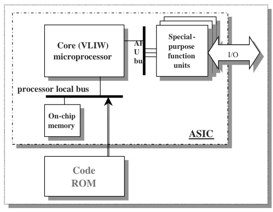
Figure 2.1 Traditional ASIC Design ... 11
Figure 2.2 Proposed Approach to Embedded System Design... 14
Figure 2.3 Zero-NOP Encoding Example ... 17
Figure 2.4 Stream-based Huffman Encoding ... 20
Figure 2.5 Tailored Encoding Example ... 22
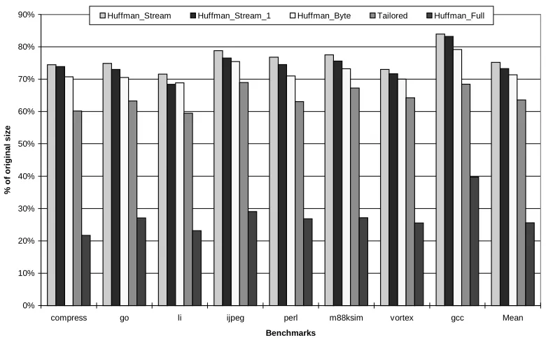
Figure 2.6 Comparison of Different Compression Techniques (code segment only). ... 23
Figure 2.7 Traditional Distribution of Miss Rate ... 27
Figure 2.8 Entropy Based Distribution... 28
Figure 2.9 Atomic Fetch Block Structure ... 29
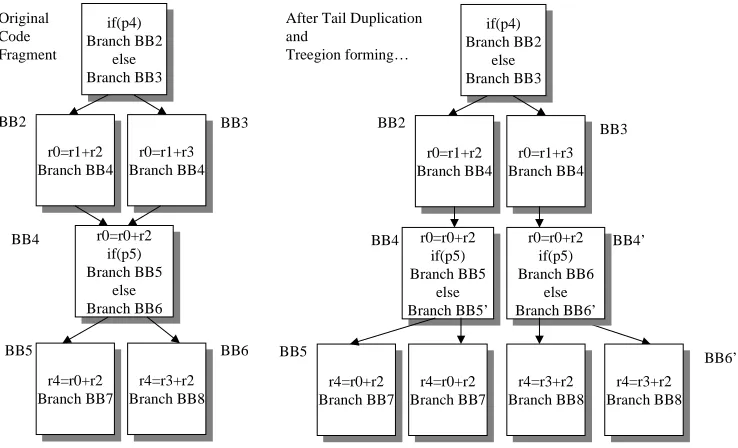
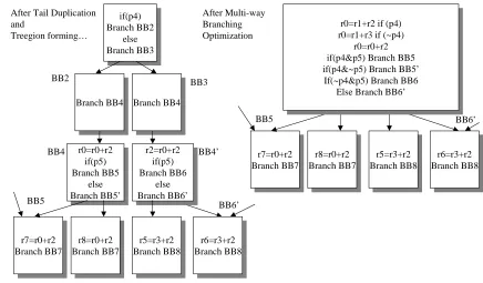
Figure 2.10 Treegion forming Example ... 31
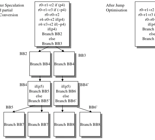
Figure 2.11 Jump Optimization Example ... 32
Figure 2.12 Multi-way Branching Example ... 33
Figure 2.13 Branch Target Randomization ... 35
Figure 2.14 ATB Miss Ratio ... 36
Figure 2.15 Compression Including ATT Size ... 39
Figure 2.16 Banked Cache Architecture ... 41
Figure 2.17 Instruction Cache Structure for Compressed Encoding ... 45
Figure 2.18 Instruction Cache Structure for the Tailored Encoding ... 46
Figure 2.19 Cache Study Summary. Instruction Delivered per Cycle... 48
Figure 2.20 Instruction Memory Bus Traffic Summary... 49
Figure 2.21 Verilog Code for Decoder Example (Custom – left, Byte Based Huffman – right) 50 Figure 2.22 The Huffman Tree Decoder Structure ... 51
Figure 2.23 Estimated Huffman Decoder Complexity... 53
Figure 2.25 Estimated to Real Size Comparison for the Byte Based, Full Compression and
Custom Coding Schemes (for the Compress Benchmark)... 55
Figure 3.1 Dynamic Compression for M88ksim... 62
Figure 3.2 Dynamic Compression for Go ... 62
Figure 3.3 Dynamic Compression for Vortex ... 63
Figure 3.4 Dynamic Compression for Gcc... 63
Figure 3.5 Dynamic Compression for Perl... 64
Figure 3.6 Dynamic Compression for Ijpeg ... 64
Figure 3.7 Dynamic Compression for Li... 65
Figure 3.8 Dynamic Compression for Compress ... 65
Figure 3.9 Summary of Data Segment Compressibility... 66
Figure 3.10 Entropy Change Due to Compression... 67
Figure 3.11 Dynamic Compression for M88ksim in presence of a Data cache ... 68
Figure 3.12 Dynamic Compression for Li in presence of a Data cache ... 70
Figure 3.13 Dynamic Compression for Perl in presence of a Data cache ... 71
Figure 3.14 Effect of Data Cache on Data Stream compressibility... 72
Figure 4.1 Traditional. Bus Encoding Experimental Setup... 74
Figure 4.2 Bus Blocks and Tuples Structure ... 75
Figure 4.3 Busy Bus Cycles ... 76
Figure 4.4 Entropy Changes due to Caching... 77
Figure 4.5 Oracle Block Distribution ... 78
Figure 4.6 Density of the Switching Activity on Compressed Data Bus ... 80
Figure 4.7 Transaction Intensity... 81
Figure 4.8 Transaction Density ... 82
Figure 5.1 Compressed Data Cache Architecture ... 85
Figure 5.2 Block Placement Example - Expanded Block Placement... 87
Figure 5.3 Block Placement Example - Reduced Block Placement... 88
Figure 5.4 Read Pipeline. Multiple Set storage... 89
Figure 5.5 Read Pipeline. Two cycle access ... 90
Figure 5.8 Logical Structure of the Reprogrammable Huffman Decoder ... 93
Figure 5.9 Dual Bank RAM Implementation of the Huffman Decoder... 94
Figure 5.10 Multiple Symbol Decoding Example... 95
Figure 5.11 Biased Huffman Tree Example... 96
Figure 5.12 Restricted Huffman Decoder Structure... 97
Figure 5.13 Profile Point Selection ... 98
Figure 5.14 Compression Dependence on Profile Point Selection. Memory side vs. Processor Side... 99
Figure 5.15 Miss Ratio Dependence on Profile Point Selection. Memory side vs. Processor Side ... 102
Figure 5.16 Compression Dependence on Profile Point Selection. Memory side vs. Storage Contents... 103
Figure 5.17 Miss Ratio Dependence on Profile Point Selection. Memory side vs. Storage Contents... 104
Figure 5.18 Two Level Compressed Data Cache ... 105
Figure 5.19 Miss Ratio for Two-Level Cache compared with the Original Implementation.... 106
Figure 5.20 Reference Hit Breakdown for the Original Compressed Data Cache... 107
Figure 5.21 Reference Hit Breakdown for the Two-Level Data Cache ... 108
Figure 5.22 Two Level Cache Size Variation (Logarithmic Scale) ... 109
Figure 5.23 Miss Ratio Comparison between Compressed and Uncompressed Caches ... 110
Figure 5.24 Absolute Dynamic Compression for Storage Profile Scheme ... 111
1 Introduction
1.1 Introduction and Motivation
The importance of embedded systems today is easy to underestimate. During the last 15
years embedded systems have grown rapidly in complexity and performance to a point where they now rival the design challenges of desktop systems. This evolutionary trend is known as
the fifth era of computing: from main frames to minicomputers to microcomputers followed by PC or desktop era and finally into the embedded system age. In the last year the number of
embedded processors sold actually exceeded the amount of general-purpose units sold. And the trend is growing. With the popularity comes the challenge. Embedded systems are now targets
for contradictory requirements: they are expected to occupy a small amount of physical space (e.g., low package count), be inexpensive, consume low power and be highly reliable. However,
they are asked to take on more complex functions [3],[17],[47]. The digital image processing, DVD and third generation cell phone base station require server-like performance from
embedded processors and most of the time they stand up to the challenge.
Regardless of the decades of intensive research and development, there are still areas that
can promise significant benefits if further researched. One such area is the quality of the data which embedded system operates upon. This includes both code and data segments of an
application. Designers spend a long time on logical optimization and minimization of
taken for data accommodation and processing. As a result, most of the time the code and data
used on embedded systems contains a significant amount of redundancy.
The presence of this redundancy would degrade the potential performance of any
processor. The Flynn’s bottleneck [32] is one of the toughest frontiers in high performance system design. It receives increasing amount of attention as the core vs. memory speed gap
multiplies. An elaborate design approaches and compiler techniques are taken to reduce this gap. Nevertheless few designers actually pay attention to the fact that information contents of
data transferred through those elaborate units is relatively low.
As the complexity and size of applications increase, the traditional method of hand
coding applications for embedded systems is quickly becoming obsolete. Although hand coding is still practiced for critical regions of a program, and is very popular for simple DSP
applications, optimizing compilers starting to play a major role in the overall process[3],[28]. But, those compilers are normally built to compile a relatively wide spectrum of applications.
So, compilers have to tolerate some redundancy in the code they produce in order to support the numerous applications encountered. For some real world applications (like the SpecInt95
benchmarks [45] compiled with the optimizing GCC compiler –O2 option for HP PA architecture) entropy ranges between 0.75 and 0.80, which means that the spilt between two possible symbols is 70 to 30%. On the other hand compilers have extensive information about
the application being compiled which could be effectively utilized.
This work presents a unified, compiler-drive approach to solving the redundancy problem.
It attempts to increase quality of the data stream that embedded systems are operating upon while preserving the original functionality. Moreover, some of the proposed methods offer
effect of high redundancy data and ultimate benefits that could be achieved by removing it.
There are three major components of embedded system front end considered in this thesis. - Instruction fetch mechanism and instruction cache design;
- System bus;
- Data fetch mechanism and data cache design;
The first part considers reduction in static size of code segment and alternative design for instruction cache. It is primarily targeted at reduction of the instruction memory size
requirements for System On Chip (SOC) architectures. It is achieved by compression or customization of the original instruction set to meet the needs of each particular application.
Several prior approaches to this problem have either defined new instruction-set architectures (e.g., the ARM Thumb Instruction Set [26] or SGI MIPS16 [27]) or defined elaborate
compression schemes without taking the impact on instruction fetch into account (e.g., IBM CodePack [9], Cooper and McIntosh [12]). The main contribution of this study is a unified,
compiler-driven approach to the problem. It presents both code compression strategies and their corresponding instruction fetch mechanisms along with compiler techniques to facilitate them.
The instruction cache is also reconsidered, and it is allowed to hold the high entropy
representation of the original code segment. This fact significantly increases instruction cache effective capacity and ultimately results in a higher performance.
The second part of this work pays attention to communication issues within the memory hierarchy and front end of embedded processors. Following many previous researches in the
area [33],[34],[49] this thesis research utilization, throughoutput and power consumption on memory and system buses in SOC. The improvement is achieved through dual coding of the
For some configurations the ultimate goal of shorter transaction time with lower switching
activity is attained.
The last, but not least, considered component is the data cache. Even with a perfect
instruction cache, a processor can only operate as fast as data could be delivered to it.
Unfortunately dynamically accessed data contains a significant amount of redundancy, which
reduces the effectiveness of the data fetch mechanism. The quality of this data could be
significantly improved by dynamic compression, if a practical scheme can be invented to exploit
this data quality. It is no surprise that dynamically accessed data is compressible. Research into value prediction hints at high rates of redundant data accesses [51]. However, exploiting this
property to yield a performance benefit has been difficult so far. With the help from compiler and the run time profiling we can double performance (miss ratio) of the data fetch path. But it
can only be truly effectively explored if the data cache is permitted to hold compressed blocks. This fact in turn introduces serious design challenges.
To summarize the proposed solutions to the above-mentioned problems it is necessary to state the following. In any embedded system, especially in those based upon the VLIW
architecture, static (or compile time) part of design cycle gains greater importance very rapidly. This offers unique opportunity to improve performance of the available hardware base with minimal dedication of some logic complexity and maximum utilization of the compile
technology. The target of optimization is the available redundancy in application. The beneficiary is the front end of an embedded system. The gain is lower physical space, higher
1.2 Previous work
1.2.1 Previous Work in Code Compression for Embedded Systems
This study would not be complete without first mentioning previous research in this area.
As was briefly mentioned in the introduction, in the past there were several studies regarding the reduction of the ROM size in an embedded system [1],[9],[10],[12],[17],[18],[47].
In several works by Wolfe, et al. [1],[17],[18], a technique to execute compressed programs on an embedded RISC architecture (MIPS was used as an example) was studied. The
initial motivation involved reducing the code size difference between the RISC and CISC embedded processors. Besides the diversity in target architecture, one of the major differences
from the current study was in the unified approach to the compression. Wolfe’s studies used the Huffman algorithm for compression, but only one common histogram was built for a set of all
experimental benchmarks and only byte-based alphabet was considered. In addition to that a fixed-size 32-byte blocks were considered an atomic unit of compression. The goal was to
create a single encoding for a fixed architecture and satisfy some range of applications. This single encoding scheme is important when building a general-purpose system, but seems less
effective for embedded applications with their unique code base. In the Wolfe’s work [1] code is uncompressed at the instruction cache miss path, and the study does not discuss further details
of instruction cache design. A special hardware structure (called Cache Line Address Lookaside Buffer) was provided to guarantee dynamic conversion between compressed and original
Several industrial solutions to the code segment size problem include the IBM CodePack
[10],[42], the ARM Thumb [26], and the SGI MIPS16 [27]. The first one uses the dictionary Huffman compression scheme, while the latter two of these provide special compact subsets of
the original instruction set architecture (ISA). Truncating the original ISA reduces its flexibility, which ultimately results in increased instruction count and, in general, slower running
applications. The CodePack also has the disadvantage of keeping the instruction cache uncompressed. The consequences of this decision are discussed in this study in great details.
Recently some design issues regarding instruction fetch mechanism for IBM’s PowerPC 405 (which uses Code Pack) were revisited by Lefurgy in [48]. The important achievement was the
fact that after certain improvement to existing hardware structures (instruction fetch pipeline architecture) the compressed code exhibit better performance then the native program.
A work by Yoshida et al. [47] specifically concentrates on low power embedded system processor design. They are using a compression method to reduce power consumption of an
embedded chip. It is specifically targeted at I/O interface by means of substituting original 32-bit instructions to a set of references in transform table (which resided on chip). This way by
execising tradeoff between silicon area and encoding complexity they significantly decrease I/O load and executable size. For ARM610 used in experiments, for some benchmarks 12-bit pseudo instructions we reported to be sufficient to substitute original 32-bit operations.
Cooper and McIntosh [12] spend most of their effort reorganizing code at the assembly level via suffix-tree code compression. They reported a very moderate level of compression (5
to 15% reduction). In either way this study is orthogonal to the approach taken in this work. A series of works by Fraser, et al. [9],[13] considers elaborate compression algorithms at
experimental results in this thesis show that neglecting instruction fetch performance in the
presence of compression may lead to incorrect conclusions about the appropriate scheme to implement.
A recent series of publications by Lefurgy [25],[43],[44] describes a way to manage the compressed code segment with software. In the [44], authors proposed software managed
decompression tightly coupled with the instruction cache. The compression granularity in [44] is a single cache line, as opposed to a single basic block used in this thesis.
An interesting study by Liao, et al. [15] employs an effective compression algorithm (External Pointer Model by Storer and Szymanski [24]) at the assembly level. In essence this
method introduces a micro procedure calls to a common regions of code. Liao reported an average of 30% code size reduction. Two implementations, software-only and ‘call-dictionary’
are considered. Both increase the number of branches in the code and (reportedly
insignificantly) the operation count. Also due to high granularity, some opportunities for
compression are missed, and as with the CodePack and many others instruction fetch schemes use decompression at miss time and uncompressed cache.
1.2.2 Previous Work in Bus Optimization
The next set of relevant research deals with bus power consumption. A number of researchers addressed power consumption on address buses. It is understandable since address
the time address (Next PC) is merely an increment of the previous value. Combined with
normally high spatial locality of references, this accounts for very low information contents. There were several researches in the area, and the most relevant are as follows. The
work by Su et al. [38] used the Gray Coding for address generation in RISC-like VLSI-BAM. The idea was to make program counter produce Gray codes as oppose to normal increment.
Certain care had to be taken of branch target addresses and reported savings were up to 58% switching activity reduction. The next work by Musol et al [41] concentrated on improving the
Address bus Gray coding by proposing a Working-Zone Encoding. This approach is based on observation that different address space areas exhibit different behavior. For some cases authors
reported up to 65% switching activity reduction.
In the domain of data buses coding the following work deserves attention. The work by
Stan and Burleson [33] concentrated on special encoding for terminated off-chip broad –level busses and tri-state on-chip buses for low-power communication. Authors considered not one
but several different techniques for minimizing transaction activity. Those methods included not only logical minimization (via compression and special coding) but also by phase
modulation of bus signals. Several techniques combining various encoding models were proposed. For their experimental setup savings of up to 68% were achieved. The same authors in [34] also proposed a Bus-Invert method which tradeoff performance and area for low power
dissipation.
1.3 Target Architecture Description
All experiments in this work are based on the TEPIC (TINKER EPIC) VLIW embedded architecture [11]. It is a 40-bit version of the HP PlayDoh VLIW machine specification [21],
adapted for embedded system use. It is important to note that the TEPIC ISA encoding is very similar to the Intel/HP 64 ISA, since the PlayDoh was one of the major influences for the
IA-64. For a core processor configuration, we assume a six-wide issue machine, with four execution units that can execute any instruction except for memory access, and two universal
units (that can perform any instruction including memory accesses). The register files are fixed to 32 general-purpose, 32 floating point and 32 predicate registers. The detailed encoding
formats for operations are shown in the Appendix Table 1.
A special compact encoding is used to encode a single VLIW Operation (MultiOP or
MOP for short – it combines all the instructions that must be issued in the same cycle). This compact encoding is known as Zero-NOP encoding and was originally designed to decrease the
size of the VLIW code segment as compared to an equivalent RISC code [7]. Each operation in the original ISA is equipped with a dedicated bit, which is set only for the last operation in a MOP (See example in Figure 2.3). This encoding allows exclusion of the empty instructions
(NOPs) in the final scheduling, which are normally the major contributors to the traditional VLIW code size explosion.
Generally speaking, TEPIC is a very powerful architecture, and a rather aggressive approach to an embedded system implementation. But with the current rate of progress,
the target architecture does not obscure the importance of the code and data compression in the
current work, which might prove even more relevant for smaller systems.
As was mentioned before, the LEGO optimizing compiler [7] is used to schedule and
optimize the code. The LEGO compiler employs standard optimizations and global instruction scheduling using Treegion [4],[5],[6] block forming. A modified version of the original
TINKER assembler is used to generate custom encoding, compressed object file as well as the synthesizeable Verilog for the decoder. The compiler is able to output an intermediate code
(Rebel) that is executed via the TINKER YULA emulation tool. Annotations are added by the compiler to emit an instruction address or load/store trace for simulations (these annotations are
not included when determining the instruction addresses or performing compression). All the studied hardware structures are modeled via simulators using an execution-driven trace.
2 Code Segment Redundancy Reduction
2.1 Motivation
The instruction fetch process is a well-known bottleneck for any architecture, and is a crucial process for embedded systems. Initial analysis shows that most of the time the
information contents in typical applications is as low as 20 -30% [50]. This means that the expensive instruction fetch mechanism 80-70% of the time performing redundant operations.
The code segment’s size can be reduced as much as 50% [50], by modifying the original ISA design and adjusting the design of the instruction cache. As a result the new program can be
executed at the same, or even faster rate, when compared to the original (native) code. By
Figure 2.1 Traditional ASIC Design
Core (VLIW) microprocessor Core (VLIW) microprocessor
On-chip memory
On-chip memory
Code ROM Code ROM processor local bus
AP U bus
ASIC Special -purpose function units
Special -purpose function units
tuning the instruction fetch pipeline, not only the performance but also the embedded system’s
overall size, cost and, indirectly, the power consumption are improved, without reducing
original functionality. The key feature is that the original ISA is uniquely adjusted for the
specific conditions of each particular application. The ISA could be either custom tailored or compressed. Once the code is compressed, it is kept this way throughout the whole instruction
fetch pipeline, from the code ROM to the decoding stage of the processor. An important and unique contribution to the previous research in this area is the fact that the instruction cache
itself is kept compressed, which significantly increases its effective capacity.
One commonly employed approach in building an embedded system is by using an
Application-Specific Integrated Circuit (ASIC) [3],[27],[28],[42] design. It is commonly known as a System On Chip (SOC). Such a system is normally composed of several building blocks
taken from a component library. All application code is stored in a ROM and an off-shelf on-chip core processor is used for execution [3],[52],[53] (see Figure 2.1). This method is a
flexible and powerful way to quick implementation of an embedded system with minimal resources. At the same time, due to the inherited flexibility, a number of high level architectural
enhancement are possible, which makes it easy to put into operation techniques and solutions described in this thesis.
First and probably the most important problem with modular ASIC approach and
off-shelf core processor is that the instruction memory ROM size multiplies with the growth of the device’s functionality. The ROM size will soon become the major cost defining factor and
bottleneck for the instruction fetch (IFetch) mechanism [1],[3],[14],[27],[28],[50] as well as overall system implementability. As a result, the code ROM often has to be implemented on a
fetching and off-die power consumption. One of the many challenges of an embedded system
design is to reduce the size of the ROM without sacrificing the functionality and performance of the system. As have been mentioned before, the approach taken in this work for the code
segment is trying to reduce redundancy of the code stored in the ROM by customizing the original ISA or by utilizing compression to modify the existing code. This increases the
utilization of the entire instruction fetch pipeline and in turn reduces the ROM size. This effect can only be achieved if a substantial amount of redundancy indeed exists in the code.
With the growth of embedded systems application complexity far beyond familiar embedded DSP applications, as have been mentioned before, the traditional methods of hand
coding and optimizing are becoming less and less effective and increasingly time consuming. In addition market’s requirements of a short design cycle and increased reliability have become a
limiting factor. A practical way to use a high level programming language, while maintaining optimal target code quality is needed [3]. This calls for developing a sophisticated compile
technology and majority of vendors invested tremendous amount of time and effort in doing that. For example, the TI 320Cxxx series of DSP processors has been successful in large part
due to the vendor-supplied optimizing compiler [28]. This work follows this trend by focusing on compiler-driven code design and data optimization for embedded systems applications. The compiler used for this study is the optimizing LEGO compiler developed in the Tinker group at
North Carolina State University (NCSU) [4],[5],[6],[11]. This is a highly optimizing speculating compiler targeted to a wide range of very long instruction word (VLIW)
architectures including the Intel IA-64 prototype. It uses Treegion-based scheduling [4],[5],[6] and provides a comprehensive set of traditional optimizations. While being a research compiler
In general an important feature of embedded systems is their specific code base. Since
an embedded system is likely to execute the same code base throughout its life span, the compiler can customize the original instruction set architecture. After scheduling and
optimization, once the final image is available, the compiler generates an efficient
custom-tailored instruction set architecture and decoder structure, which can interpret it. In other words
this study is not bounded by the rigid traditional instruction set architecture. As have been
mentioned before, traditional ISA’s are normally designed to fit a wide spectrum of applications. In this study, the instruction set architecture is a parameter and is optimized for space and cache
performance. In general the ISA could also be improved for power consumption, branch/data prediction accuracy, and various other design goals. Nevertheless only code size is considered
at this point. Another closely coupled possibility is compression of the original ISA. The result is a compressed set of original instructions that need to be uncompressed prior to execution.
The code could remain compressed all the way down to the instruction cache, with obvious advantages in the amount of required space. (See Section 2.3 for a more detailed discussion).
Figure 2.2 Proposed Approach to Embedded System Design.
Core (VLIW) microprocessor
On-chip memory
Code ROM
processor local bus
AP
U
b
u
s
ASIC Special-purpose function units
I/O
Decoder
Application
Another element of this work involves the justification of use of VLIW architectures for
embedded systems in general. Obviously the VLIW architecture seems to be a natural fit for the embedded system environment since many traditional VLIW problems do not affect embedded
systems. There is almost no code compatibility problem between generations. The use of relatively simpler hardware leads to a higher performance and low power consumption, when
compared to an equivalent issue-width superscalar architecture. And one of the foremost advantages for this work is the primary role of compiler in producing the code. Since normally
extensive information is available about the dynamic behavior of the program, high quality schedules can be produced by the optimizing compiler. All these statements were proven to be
accurate at the design of the commercial TI DSP processors [28]. The familiar challenges present are the static code size and effective high bandwidth instruction fetch. The object code
size difference between the VLIW and the superscalar architectures is first reduced by using the Zero-NOP encoding [7] and restricted code duplication in the LEGO compiler to the lower
RISC-like levels. Then the code is further optimized for required space by reduction on an individual operation size through tailor customization or compression. The instruction fetch
related issues for the Zero-NOP encoding have been discussed in [7],[8] and are further extended in this work. The decoder’s structure for the optimized encoding is produced by the compiler, which has all of the information needed – logical functionality, in- and output
connectors along with the required control signals. The overall structure of such a system is presented in Figure 2.2. Thus the compiler now plays a major role in dictating not only the
2.2 Measuring the Available Redundancy
In order to estimate the amount of useful information in a data set we should choose a way to measure the present redundancy. The available redundancy could be measured by calculating
the entropy of the code as it was defined by Shannon in [29]. In the Equation 1, Px(x) is the
probability of alphabet character x in the set. The base of the logarithm only matters for convenience of presentation and is normally set to ten.
) ( log ) ( )
(
0 ) ( ,
x Px x
Px x
H
x Px x
b
∑
≠ −
= (Equation 1)
For a binary system (see Equation 2), P is the probability of zero and 0 P is the probability of one 1
in the set (or embedded system application executable code in our case). It is also more convenient to use logarithm base two to represent results.
H =−(P0log2 P0 +P1log2P1) (Equation 2)
So for the logarithm base two, when the entropy is equal to zero this means that all probabilities but one are equal to zero (just one symbol in the set) and information contents is none. On the
other hand, when the entropy is equal to one, all symbols in the set are equally probable and the amount of information contents is at the maximum. Once it was proven that there is sufficient
redundancy (or increasing its entropy in different terms). One is the reduction of the number of
redundant assembly operations in the code [9],[12],[13],[15],[27], and the other is the reduction of the operation size [1],[10],[28]. Generally, these two approaches are both trying to achieve
the same goal – to increase the entropy of the code, but it is achieved in different ways. This means that applying both of them to the same portion of code obviously will not result in better
compression. (Nevertheless different areas of code could be optimized with different methods.) It is important to notice that this statement is assuming that all traditional optimizations (like
constant propagation, redundant computation and dead code removal) have been done and code does not contain any logically redundant operations or computations. This work chiefly
concentrates on the latter approach - reducing the operation size.
There are two methodologies for reducing operation size: tailoring the ISA or
compressing the code. The tailored ISA is a new and unique encoding, which is generated for
one particular program/application and best fits its characteristics. After decoding a tailored
Figure 2.3 Zero-NOP Encoding Example
nop nop Op_A_2 nop Op_A_4 nop nop nop
Op_B_0 nop Op_B_2 nop nop nop
nop nop nop nop
Traditional encoding
TINKER Zero-NOP encoding 0
8
16
Op_B_5 Op_B_6
Op_C_0 Op_C_2 Op_C_4 Op_C_7
0 Op_A_2 1 Op_A_4
0 Op_B_0 0 Op_B_2 0 Op_B_5 Op_B_6
0 Op_C_0 0 Op_C_2 0 Op_C_4 Op_C_7
0
2
6
Total 960bit, 560bit are in NOPs
1
1
OpType
operations are getting different sizes, which affects the branching mechanism (this topic will be
discussed in greater details in Section 2.4).
On the other hand, compression of the code segment takes an existing encoding (ISA),
and, according to the static frequencies of elements in the source code, determines the best way to pack it. Once a compressed operation is uncompressed at execution time, it still needs to be
decoded to obtain internal processor signals. Theoretically tailoring the ISA should yield better performance (e.g., no intermediate decompression needed), while compression should yield a
smaller code size. This work finds that this intuition holds, even when the improved instruction cache performance from caching compressed code is taken into account (see Section 2.7).
2.3 Code Compression Techniques
Let us first discuss compression of the original instruction set. In general, the
compression circumstances for embedded systems code segment are very favorable, since the entire code image is available statically for the compression algorithm and compression
objectives are to reduce the static size of the code. A fast hardware decoder could be used for decompression and interpretation. The main issue is the complexity, and therefore size and
speed, of the decoder. There are virtually thousands of potential compression algorithms to choose from. First, we can safely eliminate dynamic compression algorithms since we need to
store compressed code and also fully utilize its static availability. Here it is important to reemphasize that since we are concerned only with the static size of code (ROM size), we only
dynamic data sets, as we will soon see. Also if code segment would be optimizing for dynamic
interpretability, it might involve dynamic profiling and analysis. Nevertheless for the static environment, the Huffman lossless compression algorithm [2],[30] produces near optimal results
for an integer number of code bits. It is an entropy-bounded code and will use Ni =−log2 Pi
bits to encode character i in the range 1≤i≤NTotalNumberOfCharacters. It also allows reasonably fast
decompression (FSM or table lookup) at a realistic real estate price [17],[18]. For similar reasons, the Huffman compression algorithm was used in several previous studies [1],[9]. The
closest rival to the Huffman compression scheme is the Arithmetic Coding compression [55],[30],[46] algorithm (or simply arithmetic coding), which could use a fractional number of
code bits to encode the original symbol. Nevertheless, the arithmetic coding compression algorithm is much harder to decode in hardware and also might need some additional overhead
for stop symbols on a low granularity compression [46].
In addition to the described methods, a new and unique compression algorithm could be
created if a precise cost function would be defined, and this is reserved as a future work. Meanwhile for the rest of this work we will be using variations of the Huffman compression algorithm.
There were three major variations considered. They all differ in ways of composing the input alphabet for the Huffman compression algorithm. The first variation is the traditional
byte-based method [1],[2]. The code segment is treated as a stream of bytes and compressed
accordingly. As we will see shortly, this method produces the smallest decoding table and the
simplest decoder.
Second variation is the stream-based approach. The idea behind it is that certain fields
compression streams, than when combined with other fields (see Figure 2.4 and Table 2 in
Appendix). For example OpType and OpCode fields of the TEPIC operation encoding are set to ‘INT_OpType’ and ‘ADD_OpCode’ very often (up to 30% in some applications). The same is
true for the predicate field, which is most of the time (except for the if-converted code) is set to predicate register number one which in the TEPIC architecture is hard-wired to ‘true’ and means
unconditional execution of the operation. According to that observation, alphabet streams are fixed at certain operation field boundaries, as shown in Figure 2.4. The initial boundary
selection was made manually after careful examination of the generated assembly code.
Nevertheless, there were several experiments conducted in order to prove this selection and they
will be discussed shortly. However, stream based encoding is not entirely new. A similar observation was made in the IBM CodePac [10],[42] instruction set architecture and used there
as a base assumption for further Huffman table-compression scheme.
The last approach to alphabet selection for the Huffman input alphabet composition is to
Figure 2.4 Stream-based Huffman Encoding
Integer ALU Operation
Integer Compare-to-Predicate Operation
T S OPT OPCODE PREDICATE
1 1 2 5 5 5 2 8 5 1 5
T S OPT OPCODE PREDICATE
1 1 2 5 5 5 2 3 5 5 1 5 Src1 Src 2 BHWX Reserved Dest L1
Src1 Src2 BHWX D1 Reserved Dest L1
Stream 0 Stream 1 Stream 2 Stream 3
0
39
39 0
Load Operation
T S OPT OPCODE PREDICATE
1 1 2 5 5 2 2 1 2 3 5 5 1 5
consider the whole operation as a compression unit. Theoretically this alphabet might have up
to 40
2 entries (since operation size is 40 bit long), but in practice this number is significantly
smaller. This method produces the largest decoding table, but surprisingly enough, has the greatest potential for compression. This result becomes more understandable when one
examines the generated Huffman codes. Even with a large number of dictionary entries, the size of the popular ADD instruction often went down from 40 to six bits. Furthermore, none of the
Huffman codes for the full compression model has exceed the original operation size. In contrast, the maximum degree of compression of either stream approach is the sum of the
maximum compression of all (four in our case) streams, which easily exceeds six bits in most cases. From another perspective the whole operation compression method (Full Huffman from
now on) should take us as close to the entropy of the code as possible. If all possible bit combinations for all the possible instructions in the code would be determined (extract all
unique instructions), and then encoded with the least number of bits according to their absolute frequency, we will get virtually perfect (or bottom line) compression while still having separate
instructions in the code.
One additional detail of Huffman compression involves the maximum symbol length.
For some inputs, the Huffman algorithm produces very long output codes that might exceed the original operation size and become incompatible with the instruction fetch hardware (like instruction bus weight for example). The compiler keeps track of such events, and either
alternates the compression process (similar to the Bounded Huffman code described by Wolfe [1], where some additional encoding is required to guarantee the size) or substitutes the rare
2.4 Tailored Encoding
The main idea behind the Tailored encoding is to provide to an operation as much space
as it really needs in the contents of the current application, but not to compress it otherwise. At the same time we need to guarantee that within the same operation type/code instruction field
boundaries remain at fixed locations. This requirement does not impose critical limitations on size reduction but significantly simplifies the decoder. As we will soon see, the tailored
encoding method still gets significant space savings compared to the original instruction set
architecture, but avoids the intermediate decompression stage entirely. As a tailor-encoded instruction is decoded, the core processor’s internal control signals are obtained directly. In this
Figure 2.5 Tailored Encoding Example
a) Original ADD Operation
T S OPT OPCODE PREDICATE
1 1 2 5 5 5 2 8 5 1 5 Src1 Src 2 BHWX Reserved Dest L1
39 0
b) Tailored ADD Operation
T S OPCODE
1 1 6 5 5 2 5 1 Src1 Src 2 BHWX Dest L1
25 0
c) Original Store Operation
T S OPT OPCODE PREDICATE
1 1 2 5 5 5 2 2 11 1 5 Src1 Src 2 BHWX TCS Reserved L1
39 0
d) Tailored Store Operation
T OPT OPCODE
1 2 5 4 1 1 5 Src1 Src 2 L1 Dest
real hardware structure.
The algorithm for generating the Tailored encoding is rather straightforward. First, the entire code segment is ‘logically’ profiled/analyzed. The profiling information includes the
number of operations used within each operation type, the maximum number of registers simultaneously live, the size of absolute field values (like addresses and immediate values
included into operation body), and some others. If for example the application uses less than eight floating-point operations the floating point OpCode field only needs three bits. If a literal
in an immediate field of some operation exceeds some threshold value (16 bits in the current
study), this operation is separated into a Load Immediate instruction followed by the original operation with register use instead of an immediate value. Similarly, after the register
allocation, if no more than four different registers of some type are live at the same time in some source position, the source position needs only two bits to encode. The result is an
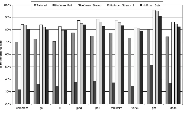
Figure 2.6 Comparison of Different Compression Techniques (code segment only).
Compression
0% 10% 20% 30% 40% 50% 60% 70% 80% 90%
compress go li ijpeg perl m88ksim vortex gcc Mean
Benchmarks
%
o
f o
rig
in
al size
uncompressed, but compact version of the original program nearly optimal for this particular
application (see Figure 2.5).
As have been mentioned at the beginning of this section, while forming the Tailored
instruction set architecture, some enhancements are possible for the decoding stage. Indeed it is a big issue, because if we overly aggressive follow the minimum requirements for operation
field we might end up with as many unique encodings (or masks) as there are different instructions in the application. That is why some size reduction needs to be sacrificed to
guarantee interpretability of the customized code. For instance, if every instruction has its Tail bit, OpType and OpCode fields (see Figure 2.5) in a fixed position (and possibly of a fixed size)
within the custom operation, decoding is significantly simplified. In addition to this, those fields could be grouped together for a MOP and placed at a certain location. Since the compiler is the
one who generates the encoding and decoder, it looks for opportunities like this when it creates the Tailored ISA.
A comparison between all of these methods is presented in Figure 2.6 for the code segment only (see Section 3.3 below for more discussion). It should also be noted that for the
stream based encoding, in addition to just choosing different fields for a stream, we could permute and combine them. This could potentially result in N! different combinations, where N is number of bits in uncompressed instruction (40 bit for the TEPIC). In order to select the
optimal stream for all the benchmarks a variation of genetic algorithm have been used. From all the considered possibilities, only six different stream configurations were selected, and the two
best performers are shown in Figure 2.6. The streams presented here were selected for the smallest average code size (stream_1) and for the smallest average decoder size (stream) among
While analyzing the compression study results, several interesting points could be noted.
The firs, and the most important one is that a significant amount of redundancy does exist in the code segment. It is quite understandable since an ISA is designed for a broad range of
applications, and the application under consideration might use only a small fraction of the presented possibilities, it is intuitive that redundancy would be present. The second obvious
conclusion is that not all compression algorithms are equally successful in removing this redundancy. The traditional byte-wise compression method could be used as a base line to
evaluate others. This algorithm views the image as a byte stream with no other considerations, which yielding an approximate 25% size reduction. The antipode of the byte-based compression
method is the Full Huffman encoding scheme, which compresses the image on an operation per operation level (40bit at a time). Note the remarkable code size reduction with the Full Huffman
compression scheme (less than 30% of original size or 70% reduction on average). As have been mentioned before, this method approaches the entropy limit of the program’s information
contents. But, as we will see in Section 2.7.3, it produces a very large decoder, which in turn might prevent the use of this algorithm as the primary compression algorithm. This fact leads us
to the final conclusion that there exists a tradeoff between the degree of compression and the complexity of the decoder. The tailored ISA approach produces code on the order of 64% of the original size, which can have favorable results for very little additional hardware overhead, so it
is represents a middle point between high complexity of decoding and low compression effectiveness.
The results presented in the Figure 2.6 neglect the branch target table overhead, which is an integral part of the compression scheme. The goal thus far has been to address the
2.5 Instruction Fetch Mechanism Issues
2.5.1 Instruction Fetch Organization and Modification of the Instruction Cache
A significant component of this work is the joint consideration of the instruction encoding and instruction fetch organization. Once original ISA has been modified the whole
instruction fetch pipeline must be adjusted. In order to interpret new instructions, the core decoder must be changed, cache design adjusted and system bus design reconsidered. All of it is
done with the help from the compiler. But most importantly of all those components, the organization of instruction cache must be reconsidered. In order to utilize the new low-entropy
encoding throughout the whole instruction fetch pipeline (and not only as ROM size-reducing
Figure 2.7 Traditional Distribution of Miss Rate
Capacity
0 0.02 0.04 0.06 0.08 0.1 0.12 0.14
1K 2K 4K 8K 16K 32K 64K 128K
technique) the instruction cache must be allowed to hold newly encoded blocks of instructions.
For simplicity of discussion let us disregard the method of encoding and just call those instructions compressed.
The fact that the instruction cache holds compressed instructions increases its capacity and, as a result, the overall throughput. It is important to stress that we are breaking a
fundamental limitation of current cache technology: the capacity miss ratio which is normally only attempted to be approached by a multi-way associativity and similar improvements. Figure
2.7 is adapted from Gee et al. [31]. The figure presents a breakdown of a miss component for caches of different associativity. The fundamental limit of a cache is compulsory (or first-seen)
misses. Compulsory misses cannot be eliminated, unless some sophisticated prefetch scheme is
used. Traditionally, the next limit was always considered the capacity misses, which only depends on the physical size of the cache storage. Finally, conflict misses are normally defeated
by a higher associativity and intelligent replacement policies.
Now with the compressed cache storage we are approaching the next fundamental limit:
Figure 2.8 Entropy Based Distribution
Capacity
EntropyCapacity
0 0.02 0.04 0.06 0.08 0.1 0.12 0.14
1K 2K 4K 8K 16K 32K 64K 128K
the entropy capacity (see Figure 2.8). In this notation, no storage is wasted due to the low
entropy of data being stored. This fact leads us to a paradoxical conclusion that we can improve the overall performance of a system by applying the compression technique, even though more
work must be done to interpret the code. A disadvantage is that the cache controller needs to be designed differently to handle the compressed contents. However, on the positive side, the
cache’s data path design is not dependent on any particular encoding and could be generalized. This independence in turn makes modular core processor design possible.
2.5.2 Program Layout
Let us now define an atomic fetch block as a sequence of instructions guaranteed (or likely to be) executed sequentially once we start execution of the first instruction in the block.
The simplest example of an atomic block is the Basic Block (a region of code with a single entry
Figure 2.9 Atomic Fetch Block Structure { A
B } BB_1:
{ C D } { E F G }
BB_2: { X
Y } { Z } BB_9:
a b
c d
f g
x y z
Alignment Boundarys (Byte Align) Random Placement
a) Original DAG b) Compressed Memory layout e f
m
At most 7 bits for Byte Aligned
Atomic Fetch Unit
x
n {...} - VLIW
and a single exit point). More sophisticated examples include a sequence of basic blocks with
no side entrances, but multiple side exits (like Superblocks [22] or Fisher-style Traces [16]). Let us consider the simplest type for now, the basic block (BB).
As have been said before, the basic block can be treated as an atomic unit of instruction
fetch (see Figure 2.9). This implies that cache can be accessed initially for only the first
operation in the basic block. After this, the cache can supply operations in a streaming (pipelined if needed) fashion, until the end of the basic block is reached. This approach is
completely transparent for the processor – it might keep on supplying each MOP address to the cache, but the cache controller does not need it to serve a miss. It starts to issue the MOP that is
only going to be requested by the processor in the next cycle. This short term ‘looking ahead’ is a valid approach for the following reasons. First, control transfer can only occur to the first
operation of a basic block (branch target). Second, a basic block should always be executed from the beginning to the end unless an interrupt has occurred, and even then its execution will
be completed after the interrupt has been handled (here subroutine calls are considered to be branches that end a basic block). All the necessary NextPC computations local to the basic
block are done within the cache, and are insignificant for the processor core, as long as correct VLIW group (MOP) is forwarded to the core decoder every cycle. Nevertheless this mechanism might be implementation specific and could depend on each particular embedded system
The use of more complicated blocks as atomic units is a matter of performance, not
correctness. If the block is permitted to have side exits, we should guarantee that they are not taken frequently (or the instruction cache will get over-polluted). This requirement is true for
superblocks [22] and Fisher-style traces [16], which are formed at compilation time with the use of profile information. But it is also true that for complex blocks some additional invalidation mechanism is needed. Nevertheless, in this study, only basic block atomic units are considered.
(Note however that the code was scheduled by first building trees of basic blocks [i.e., treegions,] and then decomposed into basic blocks after the global scheduling pass.)
2.5.3 Compiler Optimizations to Enhance Code Layout
There are a number of possible code enhancements that could be performed in order to
Figure 2.10 Treegion forming Example
r0=r0+r2 if(p5) Branch BB5 else Branch BB6 r0=r0+r2 if(p5) Branch BB5 else Branch BB6 BB2 BB4 r4=r0+r2 Branch BB7 r4=r0+r2 Branch BB7 BB5 r0=r1+r2 Branch BB4 r0=r1+r2
Branch BB4 Branch BB4r0=r1+r3 r0=r1+r3 Branch BB4 BB3 if(p4) Branch BB2 else Branch BB3 if(p4) Branch BB2 else Branch BB3 r4=r3+r2 Branch BB8 r4=r3+r2 Branch BB8 Original Code Fragment BB6 r0=r0+r2 if(p5) Branch BB5 else Branch BB5’ r0=r0+r2 if(p5) Branch BB5 else Branch BB5’ BB2 BB4 r4=r0+r2 Branch BB7 r4=r0+r2 Branch BB7 BB5 r0=r1+r2 Branch BB4 r0=r1+r2
Branch BB4 Branch BB4r0=r1+r3 r0=r1+r3 Branch BB4 BB3 if(p4) Branch BB2 else Branch BB3 if(p4) Branch BB2 else Branch BB3 r4=r3+r2 Branch BB8 r4=r3+r2 Branch BB8 After Tail Duplication
and Treegion forming… BB6’ r0=r0+r2 if(p5) Branch BB6 else Branch BB6’ r0=r0+r2 if(p5) Branch BB6 else Branch BB6’ r4=r0+r2 Branch BB7 r4=r0+r2
Branch BB7 Branch BB8r4=r3+r2 r4=r3+r2 Branch BB8
include traditional optimizations as well as some specific actions. Since VLIW architecture
chiefly depends on the compiler to achieve a high level of performance, it is essential to be aware of this matter during the scheduling.
The first enhancement is the Intelligent Code Layout to increase spatial reference locality. This optimization places the most commonly used sequences of basic blocks in close
proximity of each other in the memory. In order to determine which basic blocks are more commonly used and in which order they should be laid out, the optimization requires some
profiling information. This profile information is collected through execution of the application with some representative input data set and recording some run time statistics. The most
important of those are number of times a basic block has been executed, and order in which most executed basic blocks were visited. In addition to that, if memory paging is used, the
layout optimization also attempts to reduce the number of pages needed to execute commonly used parts of the program. This optimization increases spatial locality and is normally used to
Figure 2.11 Jump Optimization Example
if(p5) Branch BB5 else Branch BB5’ if(p5) Branch BB5 else Branch BB5’ BB2 BB4 Branch BB7 Branch BB7 BB5 Branch BB4
Branch BB4 Branch BB4Branch BB4
BB3
r0=r1+r2 if (p4) r0=r1+r3 if (~p4)
r0=r0+r2 r4=r0+r2 if(p4) r4=r3+r2 if(~p4) if(p4) Branch BB2 else Branch BB3
r0=r1+r2 if (p4) r0=r1+r3 if (~p4)
r0=r0+r2 r4=r0+r2 if(p4) r4=r3+r2 if(~p4) if(p4) Branch BB2 else Branch BB3 Branch BB8 Branch BB8 After Speculation and partial If-Conversion if(p5) Branch BB6 else Branch BB6’ if(p5) Branch BB6 else Branch BB6’ Branch BB7
Branch BB7 Branch BB8Branch BB8
BB4’
BB6’
r0=r1+r2 if (p4) r0=r1+r3 if (~p4)
r0=r0+r2 if(p4) Branch BB7
else Branch BB8
r0=r1+r2 if (p4) r0=r1+r3 if (~p4)
increase instruction cache performance and has been proven to be effective.
The next set of compile time optimization is the Jump optimization and Multi-way branching. These optimizations are related to the code layout enhancement, but are more
specific for the Treegion scheduling.
As have been mentioned before, the LEGO optimizing compiler conducts aggressive
static scheduling of VLIW code. An integral part of the scheduling process is instruction
speculation [37],[36]. Sometimes after instruction speculation by the scheduler, some basic
blocks ‘loose’ all of their instructions except for the branch (see Figure 2.10 and Figure 2.11).
This loss leads to multiple ‘back to back’ branches, which are hard to handle in the instruction fetch pipeline and often are logically redundant. Jump optimization tries to replace long chains
of jumps (with no computations in between) to shorter ones by removing redundant branch
Figure 2.12 Multi-way Branching Example
r0=r0+r2 if(p5) Branch BB5 else Branch BB5’ r0=r0+r2 if(p5) Branch BB5 else Branch BB5’ BB2 BB4 r7=r0+r2 Branch BB7 r7=r0+r2 Branch BB7 BB5 Branch BB4
Branch BB4 Branch BB4Branch BB4 BB3 if(p4) Branch BB2 else Branch BB3 if(p4) Branch BB2 else Branch BB3 r5=r3+r2 Branch BB8 r5=r3+r2 Branch BB8 After Tail Duplication
and Treegion forming… r2=r0+r2 if(p5) Branch BB6 else Branch BB6’ r2=r0+r2 if(p5) Branch BB6 else Branch BB6’ r8=r0+r2 Branch BB7 r8=r0+r2
Branch BB7 Branch BB8r6=r3+r2 r6=r3+r2 Branch BB8 BB4’ r7=r0+r2 Branch BB7 r7=r0+r2 Branch BB7 BB5 r5=r3+r2 Branch BB8 r5=r3+r2 Branch BB8 After Multi-way Branching Optimization r8=r0+r2 Branch BB7 r8=r0+r2
Branch BB7 Branch BB8r6=r3+r2 r6=r3+r2 Branch BB8
BB6’
BB6’
r0=r1+r2 if (p4) r0=r1+r3 if (~p4)
r0=r0+r2 if(p4&p5) Branch BB5 if(p4&~p5) Branch BB5’
If(~p4&p5) Branch BB6 Else Branch BB6’
r0=r1+r2 if (p4) r0=r1+r3 if (~p4)
r0=r0+r2 if(p4&p5) Branch BB5 if(p4&~p5) Branch BB5’
The multi-way branching on the other hand allows more then one branch to be executed
in a single cycle. For a VLIW architecture this branching scheme allows multiple branches a in a single VLIW instruction with priority given in left-to-right order. For control flow graph
(CFG) multiple branches translate into multiple control edges from a single basic block. Since each branch instruction has an explicit conditional register (a predicate) associated with it, the
sequence of branches is guaranteed to execute correctly. Besides obvious performance enhancement from these optimizations, they allow a reduction in the total number of basic
blocks in the program which directly correlates to the size of the static address translation tables as will be described shortly.
Standard optimizations like common subexpression elimination (CSE), strength
reduction and constant propagation [36],[37] generally contribute to logically compact code and
undoubtedly are important for the current work. For example strength reduction might substitute a complicate uncommon instruction by a sequence of simpler, more common
operations. Normally, all of these optimizations are performed prior to scheduling the code. On the other hand, in the context of code size reduction, many of the traditional
optimizations like loop peeling and unrolling [36] become less favorable. It is an important tradeoff between extracting or increasing the available instruction level parallelism (ILP) in a program and keeping the program size moderate. Since our primary goal in this study is the
2.6 Address Space Conversion
2.6.1 Branch Target Address Randomization
A critical issue for the execution of any compressed program is the change in branch
target addresses [1],[27],[42]. Every attempt to bound compressed instruction location to certain
boundaries constrains compression. For instance, if the first instruction of a basic block would be aligned to the nearest byte boundary, compression degradation will range between one and
three percent. If every instruction would be bounded, compression degradation would become unacceptable (more than ten or fifteen percent). If a high degree of compression is desired, each
option must be considered and least bounded scheme selected. Once this is accepted, it should be realized that once different instructions obtain different length of codes, the original branch
Figure 2.13 Branch Target Randomization 0000
0020 0040 0060 0080 00A0 00C0 00E0
0000 0020 0040 0060
Before Compression Aligned at 32bit addresses
unbounded compression is absolutely chaotic (see Figure 2.13). Clearly, some kind of branch
target address recalculation or translation must be performed.
First and the simplest solution is to convert the original branch targets to the compressed
targets at compilation. This process could be performed in two passes. In the first pass a new code layout and new target addresses are generated (with enough space left for later ‘plug in’ of
new targets in relative branches). On the second pass, new addresses are ‘plugged’ or ‘inserted’ into the target slots and jump tables are updated. This method is a better fit for the Tailored ISAs than for code compression schemes, because compressed code with new targets will have
to be recompressed with certain restrictions. Branch instructions could also remain uncompressed in which case a special ‘escape’ symbol should be added.
Another solution to the branch target problem is to leave the original target addresses the way they are, unchanged (just compress them along with the rest of the code) and provide a
dynamic translation mechanism at run time. This approach is very well known in general
Figure 2.14 ATB Miss Ratio
0.0% 1.0% 2.0% 3.0% 4.0% 5.0% 6.0% 7.0% 8.0%
compress go li ijpeg perl m88ksim vortex gcc Mean
Benchmark
AT
B M
iss Rat
Translation Lookaside Buffer (TLB). Similar hardware named the Cache Lookaside Buffer
(CLB) is also employed in studies by Wolfe, et al. [1],[17] and has proven to be effective. We use a similar approach to map the original address space into the compressed space with aid
from the compiler. The hardware structure is called the Address Translation Buffer (ATB) and the static table is the Address Translation Table (ATT). The ATB holds pairs of addresses,
which maps the original address space to the compressed space along with information to aid decoding, decompression and Next PC computation. The ATT has one entry for each atomic
compression block (currently a basic block). ATT is generated by the compiler and stored in memory in compressed form. The additional information stored in the ATB includes the
number of memory lines that need to be fetched in order to get the whole block, and the number of operations in the block (or simply the number of VLIW multiops in the block. Portions of the
ATT are uploaded to the ATB as needed. Due to the normally high spatial locality, the ATB has very low level of contention (see Figure 2.14) and the ATT has a tolerable static size (see Table
1). The Table 1 shows the results for Tailored instruction set encoding only. The overhead results for custom compression schemes are similar since they are not dependent on the
compression algorithm employed. Nevertheless, the ATT does add some overhead to the final storage. In general, when number of basic blocks is not optimized, the ATT adds on average 15% to the compressed size of the ROM. This fact calls for a solution to minimize its size. As
have been discussed before, the easiest way to reduce the size of ATT is to minimize the number of atomic units in the code through a compiler optimization known as the multi-way branching
(this optimization was described in greater details in section 2.5.3) or use different atomic blocks. When the multi-way branching only is performed, the total overhead of the ATT table is
granularity, the overhead could be reduced even further, but this process needs a deeper
investigation and is rserved as a future work.
ATT
Entries
ATB Miss
ratio
ATT Size
(compressed,
bytes)
Tailored ISA
Code
Segment size
Degree of
Compression
without ATT
(%)
Degree of
Compression
including ATT
(%)
compress 352 0.0016 1,223 5,260 60.16% 74.14%
go 14,036 0.0029 51,853 199,420 63.32% 79.78%
li 4,027 0.0629 12,879 44,484 59.49% 76.72%
ijpeg 8,792 0.0004 32,570 176,252 68.95% 81.69%
perl 18,130 0.0764 72,012 259,736 63.04% 80.52%
m88ksim 8,413 0.0012 30,241 148,752 67.25% 80.92%
vortex 30,699 0.0830 117,421 629,636 64.25% 76.23%
gcc 98,564 0.0842 404,664 1,468,500 68.50% 87.37%
Mean 22,877 0.0018 91,758 366,505 66.47% 83.11%
Average: 64.60% 80.05%
Briefly, at run time the ATB will provide the following information: the address of the requested block in compressed memory, the PC offset of the last operation in the block, and the
predicted PC of the following fetch block. This information is enough to fetch atomic blocks in