Efficient Computational Methods for Large Spatial Data

(1)

ABSTRACT

PARKER, RYAN JEREMY. Efficient Computational Methods for Large Spatial Data. (Under the direction of Brian J. Reich.)

Due to continued advances in technology, the ability to collect and store large data

sets are commonplace. In this dissertation we focus on spatial data collected through

technologies such as remote sensing, satellites, and computer model output. These data

are found in a variety of areas, such as research on the climate or environment, or in

areas where complex computer codes are constructed to simulate a scientific process.

The traditional methods used to analyze these data can either be very time consuming

to run on current computing platforms, or, in some cases, they can be too massive for

traditional approaches to even be considered. We propose methods that allow for efficient

computing in three different areas of spatial statistics: massive computer model output

used in climate research that is observed on a rectangular grid; estimating a nonstationary

spatial covariance observed on an irregular grid; and emulating complex computer codes

having a high-dimensional input space.

The first problem we consider is that of assessing value added within climate model

research. Climate models have emerged as an essential tool for studying the earth’s climate,

and it is common to run computationally expensive global models for study at a coarse

spatial resolution. Regional models are run with boundary conditions taken from the

global model to achieve a finer spatial scale for local analysis. These regional models add

to the computing expense, and it is of interest to know how much value the finer scale

adds over the coarser scale. We propose a new method for assessing the value added by

these higher resolution models, and we demonstrate the method within the context of

(2)

Assessment Program (NARCCAP) project. Our spectral approach using the discrete

cosine transformation (DCT) is based on characterizing the joint relationship between

observations, coarser scale models, and higher resolution models to identify how the finer

scales add value over the coarser output. The joint relationship is computed without

cumbersome matrix operations by instead estimating the smaller covariance of our data

sources at different spatial scales with a Bayesian hierarchical model. Using this model

we can efficiently estimate the value added by each data source over the others.

The second method we propose allows us to efficiently estimate nonstationary

spa-tial covariance parameters. Nonstationary covariance models require a large number

of parameters, and we develop a fused lasso approach to this problem. We do this by

partitioning the domain into a fine grid of subregions, with each subregion having a

covariance parameter. Then, we penalize the differences of these parameter values for

neighboring subregions. When the L1 norm is used to penalize the absolute differences of

parameter values, we achieve fusion that allows us to estimate stationary subdomains.

We evaluate this technique with a simulation study and demonstrate it on a data set for

tropospheric ozone in the US.

Finally, we develop a computationally efficient method for emulating the output from

deterministic computer codes within a designed experiment. By assigning observations

to blocks, we develop estimating equations that allow us to estimate Gaussian process

model covariance parameters quickly by reducing large matrix operations and exploiting

parallelization. We evaluate block assignment strategies with simulation studies for

estimation and prediction, finding that assuming independence for larger block sizes

works well for estimation. Also, we find that a subset approach for prediction should be

preferred in many cases. This approach is demonstrated on an inverse dynamics model

(3)

(4)

Efficient Computational Methods for Large Spatial Data

by

Ryan Jeremy Parker

A dissertation submitted to the Graduate Faculty of North Carolina State University

in partial fulfillment of the requirements for the Degree of

Doctor of Philosophy

Statistics

Raleigh, North Carolina

2015

APPROVED BY:

Alyson G. Wilson Christopher M. Gotwalt

Donald E. K. Martin Hua Zhou

Brian J. Reich

(5)

DEDICATION

To Nikki

For being a loving and understanding wife,

A patient and dedicated mother,

(6)

BIOGRAPHY

Ryan was born on March 10, 1983 in Charleston, South Carolina. As the son of a teacher,

his mother, Diane, gave him everything he needed early on to be a great learner. Although

he excelled in school, he taught himself how to program, and his desire to never attend

school again became strong. Because of this, he graduated high school a year early,

thinking he would never step foot in a classroom again. After high school he married his

wife, Nikki, and spent seven great years working at Northrop Grumman as a programmer,

developing software for the United States Marine Corps. But it was during this time

that he reignited his childhood love for basketball with an unexpected source: math.

This helped spark a desire to return to school, resulting in another great seven year run,

starting with attending the College of Charleston, where he earned a BS in Mathematics

in 2010. He then left his hometown of Charleston for Raleigh, North Carolina to study

statistics at North Carolina State University, where he earned a Master of Statistics

(7)

ACKNOWLEDGEMENTS

First I must thank my wife, Nikki. You have trusted and supported me from the very

beginning, when I left a good job to return to school. We have had plenty of ups and

downs during this long journey, but you have always been there for me and supported

me. And even though I still had work left to do to finish this research, you gave me the

sweetest gift of all, our precious Rory Douglas. Know that your ability to fight through

adversity and continue to endure difficult situations has not only helped us get to this

rewarding point, but also inspired me to be as strong as you are.

None of the research in this dissertation would have been possible without my advisor,

Dr. Brian Reich. Your guidance on the work here, as well as all of the other projects we

have worked together on, has helped continue my growth as a statistician. You always

seem to be available to answer any questions I have, as well as provide valuable insight

that, had I just tried it your way first, would have likely saved me a lot of time and

frustration. Thank you for everything.

Also, Steve Sain (Chapter 2), Jo Eidsvik (Chapter 3), and Chris Gotwalt (Chapter 4)

all provided guidance on one of the three projects in this dissertation. I appreciate the

time you have all taken to help with these projects, no matter how big or small.

The entire faculty and staff in the Statistics Department at NC State has been

incredible. I have been provided with incredible committee members in Dr. Alyson Wilson,

Dr. Donald Martin, and Dr. Hua Zhou. You have all provided valuable feedback to

me during the entire process. I have also had the backing of fantastic support staff in

Alison McCoy, Adrian Blue, Lanakila Alexander, Terry Byron, and Chris Waddell. This

department does so much for us all and is greatly appreciated.

(8)

Computational Statistics Fellowship. I would like to thank John Sall for funding this

opportunity. Your generosity provided me with the freedom of study few students enjoy,

and I believe I am a more well rounded statistician because of it. This fellowship has

also given me the opportunity to intern as a student statistical developer at JMP. My

manager at JMP, Chris Gotwalt, has played an important role in my statistical training.

You have given me challenging projects to work on, and when I have run into a problem

your ideas for solutions have enhanced my growth as a statistician. JMP has also given

me the opportunity to learn alongside other great statisticians, like Clay Barker, Michael

Crotty, and Laura Lancaster. Clay Barker in particular has been someone I go to often.

You seem to always have an answer for any question I ask, no matter how simple or

ridiculous it is.

I would like to thank the Mathematics Department at the College of Charleston for

giving me a great start when I returned to school. I would especially like to thank my

advisors, Dr. Martin Jones and Dr. Amy Langville. Not only did you both help me find

the area I was most interested in, statistics, but you also played a key role in preparing

me for graduate school research. Martin, your common-sense teaching style resonated well

with me, and it helped to lay a foundation that I am able to rely on when I am faced

with a difficult problem. Amy, you were always very open and encouraging of my research,

no matter the subject. Your research groups and willingness to participate in independent

studies were unparalleled.

Last, but certainly not least, I would like to thank my family and friends that provided

encouragement and support along the way. Thank you for helping me through challenging

(9)

LIST OF TABLES

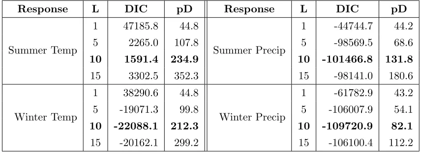
Table 2.1 DIC values and associated effective number of parameters, pD, for

models fit withL= 1,5,10,15 to each response type. Rows in bold

indicate the preferred model based on smallest DIC. . . 20

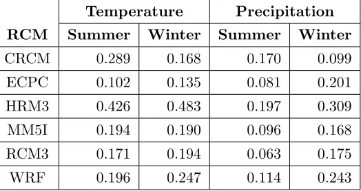
Table 2.2 The total value added (Section 2.3.3) by each RCM for the four

response types. The HRM3 performs the best in this metric in all cases, suggesting it adds the most value out of this collection of RCMs. 22

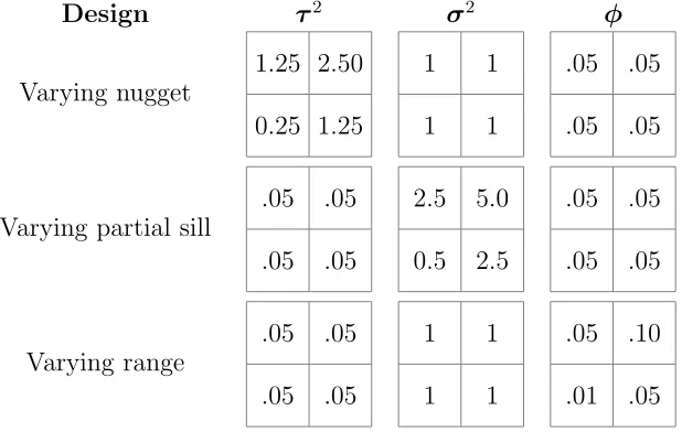
Table 3.1 Nonstationary covariance structures used to simulate data with the

nugget (left), partial sill (center), and range (right) varying by region. 38

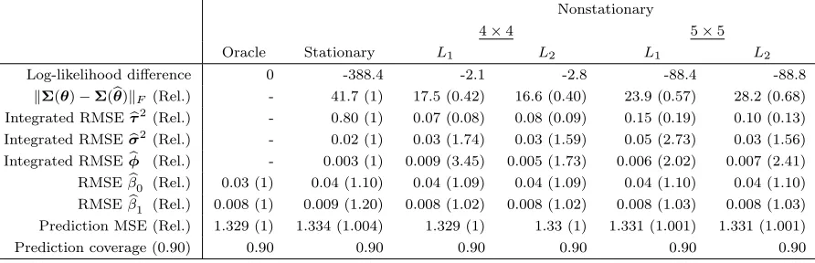
Table 3.2 Simulation study results when the nugget varies over space. The

relative factors shown in parenthesis highlight the proportional dif-ferences between the methods and the Oracle. The Oracle model uses the true values of the covariance parameters, so for metrics evaluating covariance parameters the differences are relative to the stationary model. . . 41

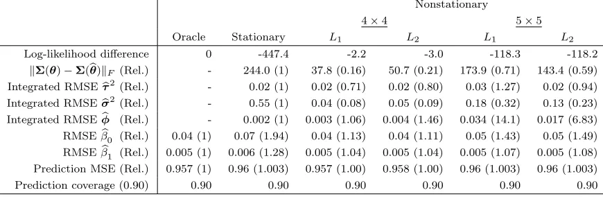
Table 3.3 Simulation study results when the partial sill varies over space.

The relative factors shown in parenthesis highlight the proportional differences between the methods and the Oracle. The Oracle model uses the true values of the covariance parameters, so for metrics evaluating covariance parameters the differences are relative to the stationary model. . . 42

Table 3.4 Simulation study results when the range varies over space. The

relative factors shown in parenthesis highlight the proportional dif-ferences between the methods and the Oracle. The Oracle model uses the true values of the covariance parameters, so for metrics evaluating covariance parameters the differences are relative to the stationary model. . . 42

Table 3.5 A comparison between the stationary (S), L1 nonstationary, andL2

nonstationary covariance models. This table compares log-likelihood of the validation set (LL) along with prediction error (Pred MSE) and prediction standard deviations (Pred SD) over sites in the val-idation set for the entire United States, excluding California, and only in California. Note the prediction MSE and SD are computed on a centered and scaled version of the original data so that the

(12)

Table 4.1 Results for n= 500 that compares the full model (Full) to assuming independent (Ind) versus dependent (Dep) blocks, with observations assigned using stratified (S) or cluster (C) assignment for a varying number of observations per block (250, 100, 50, and 25). These results compare the RMSE of parameter estimates (RM SE(bθ)), predictions

(RM SE(_by₀)), and sensitivity indices (RM SE(Sb_T)), as well as how

often the three most important inputs are selected (% Top 3) and

the time it takes to estimate parameters (Mins). . . 65

Table 4.2 Results forn = 1,000 that compares the full model (Full) to assuming independent (Ind) versus dependent (Dep) blocks, with observations assigned using stratified (S) or cluster (C) assignment for a varying number of observations per block (250, 100, 50, and 25). These results compare the RMSE of parameter estimates (RM SE(bθ)), predictions

Table 4.3 Results forn = 2,500 that compares the full model (Full) to assuming independent (Ind) versus dependent (Dep) blocks, with observations assigned using stratified (S) or cluster (C) assignment for a varying number of observations per block (250, 100, 50, and 25). These results compare the RMSE of parameter estimates (RM SE(bθ)), predictions

Table 4.4 The prediction RMSE, relative RMSE, timing, and relative timing

comparing making predictions with all of the data to our alternative methods of local prediction, independent blocks, dependent blocks, and subset prediction. The relative RMSE (b) and timings (d) are relative to the full model. . . 71

Table 4.5 Comparison of estimation timing and prediction error between the

(13)

LIST OF FIGURES

Figure 2.1 The CRU observations, NCEP reanalysis data and CRCM output

before transformation for each of the four summer/winter and

temperature (◦C)/precipitation (mm/day) responses. . . 10

Figure 2.2 Filtered data plots created by only keeping the (a) low wavenumber

data (10 or more grid boxes apart) and (b) medium wavenumber data (3 to 10 grid boxes apart). We also plot the NCEP trans-formed data (Z) versus the CRU transformed data to illustrate the

correlation between the data sources at this spatial scale. . . 13

Figure 2.3 Filtered data plots created by only keeping the (a) low wavenumber

data (10 or more grid boxes apart) and (b) medium wavenumber data (3 to 10 grid boxes apart). We also plot the CRCM trans-formed data (Z) versus the CRU transformed data to illustrate the

correlation between the data sources at this spatial scale. . . 14

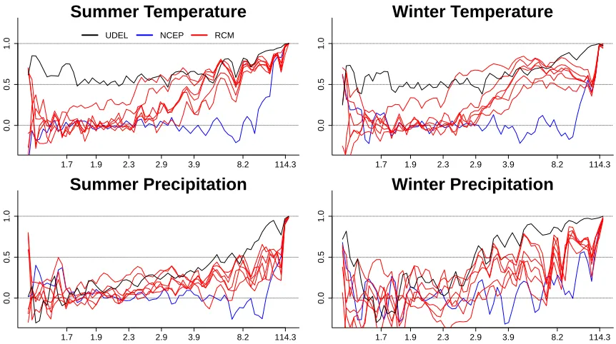
Figure 2.4 Sample correlation of the CRU data with UDEL data source (black),

NCEP data (blue), and RCMs (red) on the transformed Z scale

versus distance between grid boxes. The x-axis is in terms of grid boxes per cycle that are associated with theδ’s. . . 15

Figure 2.5 Estimated log standard deviation (pointwise 95% credible intervals

in gray) for the UDEL (solid black), CRU (dashed black), NCEP

(blue), and RCMs (red). . . 21

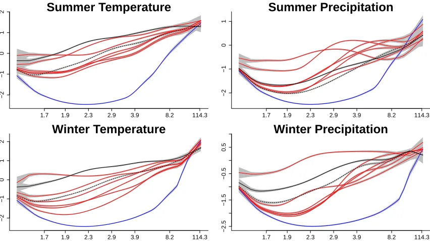
Figure 2.6 Estimated marginal correlations (joint 95% credible intervals in

gray) for CRU data with UDEL (black), NCEP (blue), and RCMs

(red) using the chosen model for each of the four response types. 22

Figure 2.7 CRU data and filtered reconstructions based on model output by

removing wavenumbers estimated to have no marginal correlation with the data. . . 23

Figure 2.8 Estimated conditional correlations (joint 95% credible intervals in

gray) for CRU data given the NCEP and an RCM using the chosen

model for each of the four response types. . . 24

Figure 3.1 Location of observations s1, . . . ,sn (a), the subregion grid having

a covariance parameter in each subregionR1, . . . ,RR (b), and the

BCL grid B1, . . . ,BB (c). . . 45

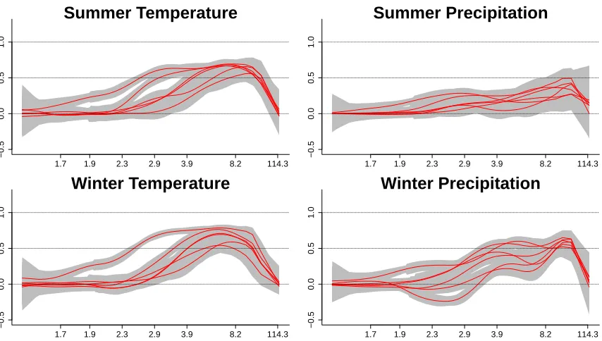
Figure 3.2 Estimated parameter values for the nugget (a), partial sill (b), and range (c) for the L1 andL2 nonstationary covariance models along

(14)

Figure 3.3 Predictions and associated prediction standard deviations (in terms of ppb) for the United States (a-b) and California (c-d) using

the stationary covariance along with the L1 and L2 regularized

nonstationary covariance models. Also included are the differences in predictions (a and c) as well as the prediction SD ratios (b and d). 50

Figure 4.1 An example of the SARCOS robot arm used to collect these

data. This SARCOS robot arm is used at the University of South-ern California Computational Learning and Motor Control lab:

http://www-clmc.usc.edu/Research/ExperimentalEquipment 73

Figure 4.2 Plots of estimated covariance parameter values for each method,

associated sensitivity indices, and a plot for the most important inputs. The covariance parameter estimates are from the residuals, and they describe the contribution of the inputs to the covariance of these residuals. The sensitivity indices are in [0,1], showing the total importance of each input to the inverse dynamics. These indices highlight the first and fourth accelerations as being the most important, and we plot the log counts ofy for each of these inputs

(15)

Chapter

1

Introduction

Modern data collection techniques, such as remote sensing, satellites, and computer model

output, make collecting massive data sets possible. These data are available in many fields,

such as climate research, environmental research, or in areas where complex computer code

can simulate a scientific process. In many of these settings the goal is to make predictions

at new locations where data is unobserved. Gaussian process models are used extensively

in these areas, as they are widely used in nonparametric regression to fit a response

surface. These Gaussian process models are ideal because they allow for flexible mean

and covariance structures to describe these data that can be used for making predictions.

Although these models work well for making these predictions, they can be difficult to

work with because of the computational limitations with large data sets.

In this chapter we introduce three spatial problems from these areas and overview

the efficient computational methods that we have developed for them. These problems

cover three different areas of spatial statistics. The first problem involves spatial data

on a rectangular grid, with multiple responses observed at each grid box. We develop a

(16)

context of climate model output. The second is the problem of estimating a nonstationary

spatial covariance model from data on an irregular grid. These models have a large

number of parameters, and we develop a method that uses variable fusion to reduce

the effective number of parameters to more efficiently estimate nonstationary covariance

parameters. Finally, we evaluate techniques for blocking observations from computer

experiments. When there are a large number of observations, blocking can dramatically

speedup the estimation of Gaussian process models for these data while maintaining

statistical efficiency for predictions and sensitivity analysis. In the sections below we

expand on each of these problems to give background for the remaining chapters.

1.1 Estimating the value added by climate models

In Chapter 2 we use climate data from the North American Regional Climate Change

Assessment Program (NARCCAP) to motivate the development of a method for evaluating

the relationship between climate model output observed on a rectangular grid in the

United States. Some of these climate models are run on a global scale, with this global

information used as inputs to models run on a finer scale. The finer scale models are more

costly to run, but they provide useful information at a finer resolution. Of interest is

evaluating how much information these finer scale models provide over the global models.

This concept is known as value added, and we gain insight into value added by estimating

the relationship between each of the climate models.

To estimate this relationship we first transform the gridded data to a wavenumber scale

using the discrete cosine transformation (DCT). This transformation removes the need for

cumbersome matrix operations and allows us to analyze subtle features in these massive

(17)

independent across resolution, we can focus on the dependence between the climate model

output at each resolution. We formulate a Bayesian hierarchical model to model this

dependence structure, and it allows us to estimate a smooth change in this relationship

over wavenumber. Using this model we can directly estimate the value added of a finer

scale model after accounting for the coarser model output. This is a unique contribution

to the study of value added by climate models.

1.2 Fusion for nonstationary covariance estimation

In spatial statistics, astationary covariance model does not change over space. That is,

the covariance between two locations only depends on their relative location. For example,

in a stationary model, two locations in the east have the same covariance if they are

simply relocated to west, as long as they have the same relative location. This is not

true for nonstationary covariance models, as they are designed to model the geographic

differences in covariance that occur in real world data. We would, for example, expect the

covariance structure for precipitation or temperature at locations in a coastal region to

differ from locations in a mountainous region.

These nonstationary spatial covariance structures are more difficult to work with

compared to the simpler stationary models due to the large number of parameters needed

to represent them. For an analysis of a large and diverse spatial domain, simplifying

assumptions such as stationarity are questionable and standard computational algorithms

are inadequate. We propose a method for efficient estimation of a nonstationary spatial

covariance using fusion in Chapter 3.

In this approach we partition the spatial domain into a fine grid of subregions and

(18)

number of parameters, and to stabilize the procedure we impose a penalty to spatially

smooth the estimates. By penalizing the absolute difference between parameters for

adjacent subregions, the solution can be identical for adjacent subregions and thus the

method identifies stationary subdomains. The method is applied to tropospheric ozone in

the US to demonstrate how the method can identify these subdomains.

1.3 Blocking observations in computer experiments

We evaluate and apply the idea of blocking observations to data from computer experiments

in Chapter 4. Deterministic computer codes can provide insight into scientific processes,

but these computer codes can be costly to run. Hence experiments are developed over the

potentially high-dimensional input space, and a sample of observations are collected for

analysis. Traditionally, Gaussian process models are built to interpolate these observations

and make predictions at untried inputs.

When, however, the number of experimental runs is large, these models are costly

to estimate. Motivated by the block composite likelihood for low-dimensional spatial

data developed by Eidsvik et al. (2014), we propose blocking observations from computer

experiments to perform efficient estimation in these situations. We evaluate how a variety

of blocking techniques perform in terms of estimation time, prediction error, and sensitivity

analysis. After identifying promising blocking techniques, we apply them to estimate an

inverse dynamics model from a 7 joint robot arm having a 21-dimensional input space and

over 40,000 observations. This is a problem that is otherwise intractable with traditional

(19)

Chapter

2

Estimating the Value Added by Regional

Climate Models

2.1 Introduction

Earth system models (ESMs) simulate weather as it responds to various forcings, including

both natural (e.g., solar or volcanoes) and anthropogenic (e.g., greenhouse gasses), over

long periods of time, and it is from these long time series that various climate properties

can be inferred. These models are continually evolving and modern ESMs not only include

components for atmosphere and ocean but also the cryosphere or land surface. While

ESMs have become invaluable tools for studying the earth’s changing climate (e.g., Stocker

et al., 2013), their relatively coarse spatial resolution hinders direct application for many

impacts studies requiring more regional and local climate information. There is also the

need to examine the role of processes that exist at finer spatial scales.

This need for higher resolution has spawned numerous approaches for downscaling

(20)

bound-ary condition data on a coarser scale. Mearns et al. (2014) offer a comprehensive review

of downscaling, including performance of both statistical approaches as well as dynamic

downscaling over North America. Statistical downscaling incorporates empirical

rela-tionships between the output from coarser models and local variables while dynamic

downscaling uses high-resolution models. Regional climate models (RCMs), for example,

can achieve much higher resolution but only on a limited spatial domain and require

time-dependent lateral boundary conditions from a global dataset.

Mearns et al. (2014) point out that one of the key issues when considering downscaling

approaches is added value (Flato et al., 2013, Section 9.6.4), which is the additional climate

information that is gained from employing an RCM or other type of downscaling. A number

of papers have addressed value added by examining biases or correlations (e.g., Pr¨ommel

et al., 2010; Feser et al., 2011; Racherla et al., 2012). Others have created new measures

to assess added value. Feser (2006) examines spatial correlations on different spatial scales

while Paeth and Mannig (2013) adapt an optimal fingerprint technique. Kanamitsu and

de Haan (2011) create an added value index based on spatial characteristics while Di

Luca et al. (2012, 2013) examine an index based on a type of a variance decomposition.

In this chapter we propose a new method for assessing value added. Our approach is

to decompose the data into different spatial scales, and then model the joint relationships

between data sources at each scale using a Bayesian hierarchical model. Using this joint

relationship, we evaluate the value added in three ways, with (1) the marginal correlations

between the RCM output and observations, (2) the conditional correlation between the

RCM output and observations after accounting for the coarser output, and (3) a measure

of the total value added using these conditional correlations (see Section 2.3.3). In our

analysis of data from the North American Regional Climate Change Assessment Program

(21)

and RCMs. Like Feser (2006), we use a multi-resolution spectral approach to analyze these

relationships. This allows us to assess the value added by RCMs separately by spatial

scales, e.g., global, regional, and local scales. Our approach differs from Feser (2006) in

several ways. First, rather than studying correlation between RCMs and the observations

at different spatial scales, we study the correlation between RCMs and the observations

conditional on the driving reanalysis data. This allows us to more directly assess the value

added by the RCM in terms of signal that can be explained by the RCM but not the

coarser information. In addition, our fully Bayesian approach allows us to quantify the

uncertainty of the value added by RCMs and hence perform formal statistical inference.

This chapter proceeds as follows. In Section 2.2 we introduce the NARCCAP data

that we will use to assess the value added by RCMs. For our study we summarize this

data to be the average temperature and precipitation values over summer and winter.

The methodology we use to assess added value is described in Section 2.3. In this section

we review the discrete cosine transformation (DCT) and the hierarchical model we use to

analyze the transformed data. In addition, we describe how we assess value added with

this model. We analyze the NARCCAP data with our method in Section 2.4 and conclude

with a discussion in Section 2.5.

2.2 Data

To illustrate our approach to assessing added value, we analyze data from the North

American Regional Climate Change Assessment Program (Mearns et al., 2009). NARCCAP

is a large-scale program using multiple RCMs and multiple GCMs to produce regional

climate change projections over North America and to examine the uncertainties in these

(22)

Regional Spectral Model (UC San Diego/Scripps; Juang et al., 1997) 2) CRCM: Canadian

Regional Climate Model (Canadian Centre for Climate Modelling and Analysis; Caya and

Laprise, 1999), 3) RCM3: Regional Climate Model version 3 (Abdus Salam International

Center for Theoretical Physics; Giorgi et al., 1993a, Giorgi et al., 1993b, Pal et al.,

2000, Pal and Coauthors, 2007), 4) WRF: NCAR Weather Research and Forecasting

model (National Center for Atmospheric Research; Skamarock et al., 2005), 5) MM5I:

NCAR/PSU Mesoscale Model 5 (National Center for Atmospheric Research/Pennsylvania

State University; Grell et al., 1993), and 6) HRM3: Hadley Regional Model 3 (Met

Office Hadley Centre; Jones et al., 2003). In Phase I of NARCCAP (Mearns et al.,

2012), boundary conditions were provided by the global NCEP-DOE Reanalysis 2 dataset

(Kanamitsu et al., 2002). Phase II of NARCCAP (Mearns et al., 2013) used boundary

conditions from four different GCMs to provide both a 30-year current (1970-2000) and

a 30-year future (2040-2070) ensemble of model output. The future runs use the A2

emissions scenario (Nakicenovic et al., 2000).

Our focus here is on the output from Phase I. In particular, we analyze the mean

surface temperature and precipitation for the summer and winter over the span of 20-years

(1980-2000). These means are computed over the days in the months of the summer

(June, July, and August) and winter (December, January, and February) during this

20-year time period. For comparison, we use version 2.01 of the University of Delaware

(UDEL) temperature and precipitation values (Willmott and Matsuura, 1995) as well as

version 2.10 Climatic Research Unit (CRU) temperature and precipitation values (Mitchell

and Jones, 2005) from the summer and winter. We use both the UDEL and CRU data

because there are often differences that arise due to differences in the data sources or

methodologies used when creating these reconstructions.

(23)

data are interpolated to a common 50km grid mesh. For convenience, this grid is the same

as the CRCM model. Data were interpolated using thin plate splines (McGinnis et al.,

2010; Loikith et al., 2014, Section 5b), a kriging algorithm implemented in thefastTps

routine (Fields Development Team, 2006). CRU and UDEL data sets were interpolated

similarly. Thin plate splines, and splines in general, are well-studied tools for interpolation

and smoothing; see, for example, Green and Silverman (1994).

Reanalysis combines observations from many different sources and numerical models

to produce spatially and temporally complete datasets. The NCEP-DOE Reanalysis 2

(Kanamitsu et al., 2002) corrects a number of errors in the NCEP-NCAR Reanalysis 1

(Kalnay et al., 1996), and, as Mearns et al. (2009) notes, using this data set for boundary

conditions is an approximation to using actual observations, if such would actually exist, to

drive the regional models. This reanalysis has a 2.5 x 2.5 degree resolution (approximately

250km).

Figure 2.1 plots a subset of the data sources to illustrate the differences between the

observational data, NCEP reanalysis, and RCM output (CRCM was arbitrarily chosen

simply to highlight the general differences for RCMs). We can see from these plots that

the NCEP reanalysis is smoother than the RCM output, and we are interested in knowing

how much more added information the RCMs bring over this driving reanalysis, as the

RCMs appear to identify more small-scale features.

2.3 Methodology

In this section we describe the methodology we use to characterize the joint relationship

of the observational data, driving reanalysis, and RCM output. We will let Y be the

(24)

Summer Temp: CRU Data

10 15 20 25 30

NCEP

10 15 20 25 30

CRCM RCM

10 15 20 25 30

Winter Temp: CRU Data

−10 0 10 20

NCEP

−10 0 10 20

CRCM RCM

−10 0 10 20

Summer Precip: CRU Data

2 4 6 8 10

NCEP

2 4 6 8 10

CRCM RCM

2 4 6 8 10

Winter Precip: CRU Data

2 4 6 8 10 12

NCEP

2 4 6 8 10 12

CRCM RCM

2 4 6 8 10 12

Figure 2.1: The CRU observations, NCEP reanalysis data and CRCM output before

transformation for each of the four summer/winter and temperature (◦C)/precipitation

(25)

(described in Section 2.2) from one of the observational, driving reanalysis, or RCM data

sources, where Y(i, j) is the value in row i and column j. In Section 2.3.1 we review the

discrete cosine transformation, which we use to perform an orthogonal transformation on

Y to obtain Z so that we have data on a scale that is more tractable to work with. Using

this transformed data we formulate a Bayesian hierarchical model (Section 2.3.2) for

modeling the covariance between each of our data sources at each resolution. We conclude

by outlining the techniques we use to summarize this covariance and assess added value

in Section 2.3.3.

2.3.1 Discrete cosine transformation

Rather than model the data sources directly, we transform Y to Z using the

two-dimensional discrete cosine transformation (DCT, Ahmed et al., 1974). This transformation

allows us to isolate signals at different spatial scales. Our motivation for choosing the

DCT over the fast Fourier transformation comes from the DCT’s close connection to the

common spatial statistical model for gridded data, as described below in Section 2.3.2.

More importantly, Denis et al. (2002) demonstrate that the DCT is preferred for the

atmospheric fields we are working with because of their aperiodic structure.

The DCT transforms Y toZ with

Z(m, n) =ambn N1−1

X

i=0

N2−1

X

j=0

cos

π m

N1

i+1

2

cos

π n

N2

j+ 1

2

Y(i, j), (2.1)

form= 0, . . . , N1−1 andn= 0, . . . , N2−1, wheream = 1/

√

N1ifm= 0 andam =

p

2/N1

if m >0, and bn= 1/

√

N2 if n = 0 and bn=

p

2/N2 if n > 0. EachZ(m, n) is a linear

combination of the data that measures the signal with a different spatial wavenumber. The

(26)

corresponds to the average of the columns of Y (representing the longitudes) formed by the linear combination with coefficients that are a cosine with period 2N2/n. Z(m, n)

corresponds to the feature with wavenumber ω = (ω1, ω2), where ω1 = m/(2N1) is the

one-dimensional wavenumber in the latitudes and ω2 =n/(2N2) is the one-dimensional

wavenumber in the longitudes. These correspond to periods 2N1/m in the latitudes and

2N2/n in the longitudes.

To illustrate how the transformation can allow us to examine data at different spatial

scales, we plot filtered data over the ranges of grid boxes per cycle of greater than 10 (low

wavenumbers) and between 3 and 10 (medium wavenumbers). These plots for summer

temperature and the NCEP data are shown in Figure 2.2, and Figure 2.3 shows these for

the CRCM model output. These show that at medium wavenumbers the CRCM model

output continues to have a positive correlation with the observation data. The NCEP,

however, does not have such a relationship and is uncorrelated. At low wavenumbers we

observe that the differences are higher in the west between the NCEP and the observed

data compared to the differences between the observed data and the CRCM. It is also

interesting to see that both the NCEP reanalysis data and CRCM model output are

higher in the midwest region.

2.3.2 Bayesian hierarchical model

In this section we propose a statistical model for modeling the covariance between our

K = 9 data sources. This covariance is used to examine and quantify the value added by

RCMs. To illustrate one component of this covariance, we plot the empirical correlations

of the transformed CRU data with the UDEL data, NCEP data and RCM output in

Efficient Computational Methods for Large Spatial Data

ABSTRACT

DEDICATION

BIOGRAPHY

ACKNOWLEDGEMENTS

TABLE OF CONTENTS

LIST OF TABLES

LIST OF FIGURES

Chapter

1

Introduction

1.1

Estimating the value added by climate models

1.2

Fusion for nonstationary covariance estimation

1.3

Blocking observations in computer experiments

Chapter

2

Estimating the Value Added by Regional

Climate Models

2.1

Introduction

2.2

Data

2.3

Methodology

2.3.1

Discrete cosine transformation

2.3.2

Bayesian hierarchical model