Machine Learning Models for Sales Time Series Forecasting

(1)

Machine Learning Models for

Sales Time Series Forecasting

Bohdan M. Pavlyshenko

SoftServe, Inc., Ivan Franko National University of Lviv

* Correspondence: [email protected], [email protected]

Version November 5, 2018 submitted to Preprints

Abstract: In this paper, we study the usage of machine learning models for sales time series 1

forecasting. The effect of machine learning generalization has been considered. A stacking approach 2

for building regression ensemble of single models has been studied. The results show that using 3

stacking technics, we can improve the performance of predictive models for sales time series 4

forecasting. 5

Keywords: machine learning; stacking; forecasting; regression; sales; time series 6

1. Introduction 7

Sales prediction is an important part of modern business intelligence. It can be a complex problem. 8

Especially, in the case of lack of the data, missing data, a lot of outliers. Sales can be treated as a 9

time series. At present time different time series theories and models have been developed. We can 10

mention Holt-Winters model, ARIMA, SARIMA, SARIMAX , GARCH, etc. But their use in case of 11

sales prediction is problematic due to several reasons. Here are several of them: 12

• We need to have historical data for a long time period to capture seasonality. But often we do not 13

have historical data for a target variable, for example in case when a new product is launched. 14

But we have sales time series for a similar product and we can expect that our new product will 15

have a similar sales pattern. 16

• Sales can have complicated seasonality - intra-day, intra-week, intra-month, annual. 17

• Sales data can have a lot of outliers and missing data. We have to clean outliers and interpolate 18

data before using a time series approach. 19

• We need to take into account a lot of exogenous factors which have impact on sales. 20

Sales prediction is rather a regression problem than a time series problem. Practice shows that the 21

use of regression approaches can often give us better results comparing with time series methods. 22

Machine learning algorithms make it possible to find patterns in the time series. In papers [1–3], we 23

study different approaches for time series modeling such as using linear models, ARIMA algorithm, 24

XGBoost machine learning algorithm. 25

One of the main assumptions of regression methods is that the patterns in the past data will be 26

repeated in future. In the sales data, we can observe several types of patterns and effects. They are: 27

trend, seasonality, autocorrelation, patterns caused by the impact of such external factors as promo, 28

pricing, competitors behavior. We also observe noise in the sales. Noise is caused by the factors which 29

are not included into our consideration. In the sales data, we can also observe extreme values - outliers. 30

If we need to perform risk assessment, we need to take into account noise and extreme values. Outliers 31

can be caused by some specific factors, e.g. promo events, price reduction, weather conditions, etc. 32

If these specific events are repeated periodically, we can add a new feature which will indicate these 33

special events and describe the extreme values of the target variable. 34

In this study, we consider the usage of machine learning models for sales time series forecasting. 35

(2)

2 of 10

2. Machine Learning Predictive Models 36

For our analysis, we used store sales historical data from “Rossmann Store Sales” Kaggle 37

competition [4]. These data represent the sales time series of Rossmann stores. Calculations were 38

conducted in the Python environment using the main packagespandas, sklearn, numpy, keras, matplotlib, 39

seaborn. To conduct analysis,Jupyter Notebookwas used. 40

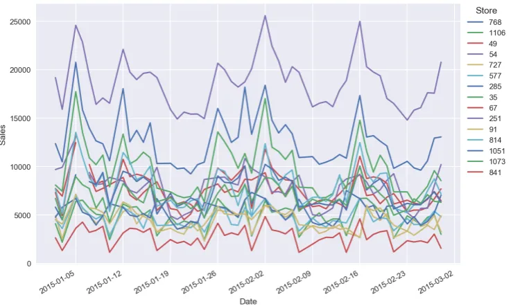
Figure1shows typical time series for sales. On the first step we conducted the descriptive

Figure 1.Typical time series for sales 41

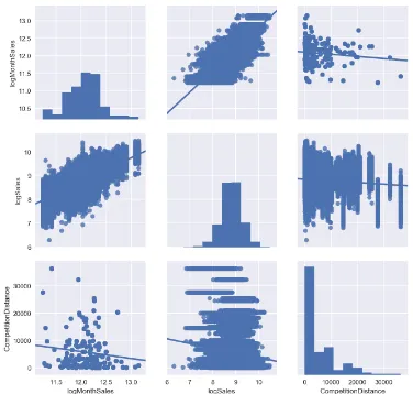
analytics, which is a study of sales distributions, data visualization with different pairplots. It is helpful 42

in finding correlations and sales drivers on which we can concentrate our attention. The figures2,3,4 43

show the results of the descriptive analytics.

Figure 2.Boxplots for sales distribution vs day of week 44

Supervised machine learning methods are very popular. Using these methods, we can find 45

complicated patterns in the sales dynamics. Some of the most popular are tree based classifiers, e.g. 46

Random Forest and XGBoost, etc. A specific feature of tree based methods is that they are not sensitive 47

to monotonic transformations of the features. It is very important when we have a set of features 48

with different nature. For example, one feature represents promo, another - competitors’ prices, 49

macroeconomic trends, customers’ behavior. A specific feature of most machine learning methods is 50

that they can work with stationary data only. We cannot apply machine learning to non-stationary 51

Preprints (www.preprints.org) | NOT PEER-REVIEWED | Posted: 5 November 2018 doi:10.20944/preprints201811.0096.v1

(3)

Figure 3.Factor plots for aggregated sales

sales with a trend. We have to do detrending of time series before applying machine learning. In 52

case of small trend, we can find bias using linear regression on the validation set. Let us consider the 53

supervised machine learning approach using sales historical time series. For the case study, we used 54

Random Forest algorithm. As covariates, we used categorical features: promo, day of week, day of 55

month, month. For categorical features, we applied one-hot encoding, when one categorical variable 56

was replaced by n binary variables, where n is the amount of unique values of categorical variables. 57

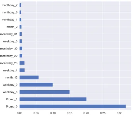
Figure5shows the forecasting for sales time series using of Random Forest algorithm. Figure6shows 58

the feature importance. For error estimation, we used a relative mean absolute error (MAE) which 59

is calculated aserror=MAE/mean(Sales)·100% . Figure7shows forecast residuals for sales time 60

series, Figure8shows the rolling mean of residuals, Figure9shows the standard deviation of forecast 61

residuals. 62

In the forecast, we may observe bias on validation set which is a constant (stable) under- or 63

over-valuation of sales when the forecast is going to be higher or lower with respect to real values. It 64

often appears when we apply ML methods to non-stationary sales. We can conduct the correction of 65

bias using linear regression on the validation set. We have to differentiate the accuracy on a validation 66

set from the accuracy on a training set. On the training set, it can be very high but on the validation set 67

it is low. The accuracy on the validation set is an important indicator for choosing an optimal number 68

of iterations of ML algorithm. 69

3. Effect of Machine Learning Generalization 70

The effect of machine learning generalization consists in the fact that a classifier captures the 71

patterns which exist in the whole set of stores or products. If the sales have expressed patterns, then 72

generalization enables us to get more precise results which are resistant to sales noise. It also gives us 73

an ability to make prediction in case of very small number of historical sales data, which is important 74

when we launch a new product or store. In the case study of machine learning generalization, we 75

(4)

4 of 10

Figure 4.Pair plots with log(MonthSales), log(Sales), CompetitionDistance

for specified time period of historical data, state and school holiday flags, distance from store to 77

competitor’s store, store assortment type. Figure10shows the forecast in the case of historical data 78

with a long time period (2 years) for a specific store, Figure11shows the forecast in the case of historical 79

data with a short time period (3 days) for the same specific store. In case of short time period, we can 80

receive even more precise results. If we are going to predict the sales for new products, we can make 81

expert correction by multiplying the prediction by a time dependent coefficient to take into account 82

the transient processes, e.g. the process of product cannibalization when new products substitute other 83

products. 84

4. Stacking of Machine Learning Models 85

Having different predictive models with different sets of features, it is useful to combine all these 86

results into one. There are two main approaches for such a purpose - bagging and stacking. Bagging is 87

a simple approach when we make weighted blending of different model predictions. Such models 88

use different types of classifiers with different sets of features and meta parameters, then forecasting 89

errors will have a weak correlation and they will compensate each other under the weighted blending. 90

Forecasting errors of these models will be of weak correlation and these errors will be compensated by 91

each other under the weighted blending. The less is the error correlation of model results, the more 92

precise forecasting result we will receive. Let us consider the stacking technic [5] for building ensemble 93

of predictive models. In such an approach, the results of predictions on the validation set are treated 94

as input regressors for the next level models. As the next level model, we can consider a linear model 95

or another type of a classifier, e.g. Random Forest classifier or Neural Network. It is important to 96

(5)

Figure 5.Sales forecasting (train set error:3.9%, validation set error: 11.6%)

Figure 6.Features importance

mention that in case of time series prediction, we cannot use a conventional cross validation approach, 97

we have to split a historical data set on the training set and validation set by using time splitting, so the 98

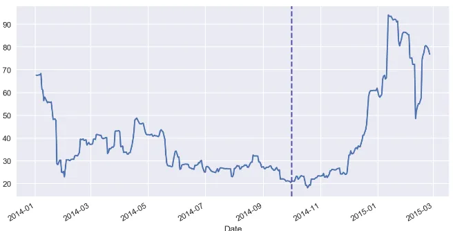
training data will lie in the first time period and the validation set - in the next one. Figure12shows 99

the time series forecasting on the validation sets obtained using different models. Vertical dotted line 100

on the Figure12separates validation set and out-of-sample set which is not used in the model training 101

and validation processes. On the out-of-sample set, one can calculate stacking errors. Predictions on 102

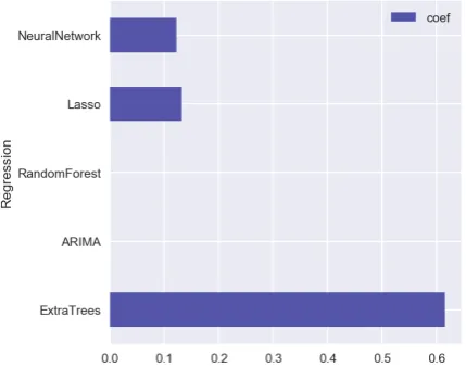
the validation sets are treated as regressors for the linear model with Lasso regularization. Figure13 103

shows the results obtained on the second-level Lasso regression model. Only three models from the 104

first level (ExtraTree, Lasso, Neural Network) have non zero coefficients for their results. For other 105

cases of sales datasets, the results can be different when the other models can play more essential role 106

in the forecasting. Table1shows the errors on the validation and out-of-sample sets. These results 107

(6)

6 of 10

Figure 7.Forecast residuals for sales time series

Figure 8.Rolling mean of residuals

Figure 9.Standard deviation of forecast residuals

(7)

Figure 10.Sales forecasting with long time (2 year) historical data, error=7.1%

(8)

8 of 10

Figure 12.Time series forecasting on the validation sets obtained using different models

Figure 13.Stacking weights for regressors

(9)

Table 1.Forecasting errors of different models

Model Validation error Out-of-sample error

ExtraTree 14.6% 13.9%

ARIMA 13.8% 11.4%

RandomForest 13.6% 11.9%

Lasso 13.4% 11.5%

Neural Network 13.6% 11.3%

Stacking 12.6% 10.2%

To get insights and to find new approaches, some companies propose their analytical problems 109

for data science competitions, e.g. at Kaggle [6]. The company Grupo Bimbo organized a Kaggle 110

competition Grupo Bimbo Inventory Demand [7]. In this competition, Grupo Bimbo invited Kagglers 111

to develop a model to forecast accurately the inventory demand based on historical sales data. I had 112

a pleasure to be a teammate of a great team ’The Slippery Appraisals’ which won this competition 113

among nearly two thousand teams. We proposed the best scored solution for sales prediction in more 114

than 800,000 stores for more than 1000 products. Our first place solution is at [8]. To build our final

XGBoost Model 1 XGBoost Model 2 Classifier m Model n Linear Model ExtraTree Model Neural Network Model w1ET+w2LM+w3N N

... Level 1

Level 2 Level 3

Figure 14.Mulitlievel machine learning model for sales time series forecasting 115

multilevel model, we exploited AWS server with 128 cores and 2Tb RAM. For our solution, we used 116

a multilevel model, which consists of three levels (Figure14). We built a lot of models on the 1st 117

level. The training method of most 1st level models was XGBoost. On the second level, we used a 118

stacking approach when the results from the first level classifiers were treated as the features for the 119

classifiers on the second level. For the second level, we used ExtraTrees classifier, the linear model 120

from Python scikit-learn and Neural Networks. On the third level, we applied a weighted average 121

to the second level results. The most important features are based on the lags of the target variable 122

grouped by factors and their combinations, aggregated features (min, max, mean, sum) of the target 123

variable grouped by factors and their combinations, frequency features of factors variables. One of 124

the main ideas in our approach is that it is important to know what were the previous week sales. If 125

during the previous week too many products were supplied and they were not sold, next week this 126

product amount, supplied to the same store, will be decreased. So, it is very important to include 127

lagged values of the target variable as a feature to predict next sales. More details about our team’s 128

winer solution are at [8]. The simplified version of the R script is at [9]. 129

5. Conclusion 130

In our case study, we considered different machine learning approaches for time series forecasting. 131

The accuracy on the validation set is an important indicator for choosing an optimal number of 132

(10)

10 of 10

classifier captures the patterns which exist in the whole set of stores or products. It can be used for 134

sales forecasting when there is a small number of historical data for specific sales time series in the case 135

when a new product or store is launched. Using stacking model on the second level with the covariates 136

that are predicted by machine learning models on the first level, makes it possible to take into account 137

the differences in the results for machine learning models received for different sets of parameters and 138

subsets of samples. For stacking machine learning models the Lasso regression can be used. Using 139

multilevel stacking models, one can receive more precise results in comparison with single models. 140

References 141

1. Pavlyshenko, B. M. Linear, machine learning and probabilistic approaches for time series analysis. In IEEE 142

First International Conference on Data Stream Mining & Processing (DSMP), Lviv, Ukraine, pp. 377-381, 143

August 23-27, 2016. 144

2. Pavlyshenko, B. Machine learning, linear and bayesian models for logistic regression in failure detection 145

problems. In IEEE International Conference on Big Data (Big Data), Washington D.C., USA, pp. 2046-2050, 146

December 5-8, 2016. 147

3. Pavlyshenko, B. Using Stacking Approaches for Machine Learning Models. In 2018 IEEE Second International 148

Conference on Data Stream Mining & Processing (DSMP) , Lviv, Ukraine, pp. 255-258, August 21-25, 2018. 149

4. ’Rossmann Store Sales’, Kaggle.Com, URL: http://www.kaggle.com/c/rossmann-store-sales . 150

5. Wolpert, D. H. Stacked generalization. Neural networks, 5(2), pp. 241-259,1992. 151

6. Kaggle: Your Home for Data Science. URL: http://kaggle.com 152

7. Kaggle competition ’Grupo Bimbo Inventory Demand ’ URL: https://www.kaggle.com/c/grupo-bimbo-inventory-demand 153

8. Kaggle competition ’Grupo Bimbo Inventory Demand’ #1 Place Solution of The Slippery Appraisals team. 154

URL:https://www.kaggle.com/c/grupo-bimbo-inventory-demand/discussion/23863 155

9. Kaggle competition ’Grupo Bimbo Inventory Demand’ Bimbo XGBoost R script LB:0.457. URL: 156

https://www.kaggle.com/bpavlyshenko/bimbo-xgboost-r-script-lb-0-457 157