A distributed virtual MIMO coalition formation framework for energy efficient wireless networks

R E S E A R C H

Open Access

A distributed virtual MIMO coalition formation

framework for energy efficient wireless

networks

Rodrigo A Vaca Ramirez

, John S Thompson

, Eitan Altman

and Victor Ramos

Abstract

In this paper, we consider a distributed virtual multiple-input multiple-output (MIMO) coalition formation algorithm. Energy savings are obtained in the reverse link by forming multi-antenna virtual arrays for information transmission. Virtual arrays are formed by finding a stable match between two sets of single antenna devices such as mobile stations (MSs) and relay stations (RSs) based on a game theoretic approach derived from the concept of the college admissions problem. Thus, power savings are obtained through multi-antenna arrays by implementing the concepts of spatial diversity and spatial multiplexing for reverse link transmission. We focus on optimizing the overall consumed power rather than the transmitted power of MSs and RSs. Furthermore, it is shown analytically and by simulation that when the overall consumed power is considered, the energy efficiency of the single antennas devices is not always improved by forming a virtual MIMO array. Hence, single antenna devices may prefer to transmit on their own when channel conditions are favorable. In addition, the simulation results show that the framework we propose provides comparable energy savings and a lower implementation complexity when compared to a centralized exhaustive search approach.

Keywords: Game theory; Energy efficiency; Distributed decision making; MIMO

1 Introduction

Energy consumption has become a major research topic due to the growing energy costs which comes along with the global increase in the number of mobile subscribers. On one hand, the data volume of communication net-works is expected to grow by a factor of 10 every 5 years, which brings a doubling of energy consumption over the same time period [1,2]. On the other hand, mobile sta-tions’ (MSs) capabilities and operation time are mostly constrained due to their limited battery resources. Most of the power expenditure of MSs in transmission mode is due to the power amplifiers and the signal process-ing module [3]. Thus, effective solutions allowprocess-ing MSs to maximize their battery life while optimizing the overall power expenditure rather than only the transmit power are an open research field [1,4-6].

The use of multiple antennas in wireless links has emerged as an effective way to reduce the power

con-*Correspondence: [email protected]

1Scientific Division, Federal Police, 01110, Constituyentes 947, Mexico City, Mexico

Full list of author information is available at the end of the article

sumption in the reverse link. It has been shown in [7] that multi-antenna systems require less transmitted power to achieve the same capacity requirements than single antenna devices. In Long-Term Evolution (LTE), a base station (BS) may support multiple antennas. However, MSs may not be equipped with more than one single antenna due to physical constraints [8,9]. Hence, imple-menting effective solutions allowing MSs to benefit from the advantages of multi-antenna systems without the extra burden of having multiple antennas physically present at the users’ side has become a major issue for current communication systems.

Cooperative communications have recently attracted significant attention as an effective way to improve the performance of wireless networks [10,11]. By the use of cooperative techniques, wireless devices are allowed to share and use the network resources in a more effi-cient way [6,10,12-16]. As an example, the authors in [14] present a cooperative method to share the network resources and manage interference among femtocells in a distributed manner. Hence, femtocells form coalitions to improve their performance by sharing spectral resources

and maximizing the spatial reuse. In [16], the authors con-sider the consequences that arise when two multi-antenna systems share the same spectrum band. They demonstrate that if cooperation between the two systems is possible, they may achieve a performance close to the maximum sum-rate.

An important application of cooperative techniques is the formation of virtual multi-antenna arrays. In this context, a number of single antenna devices may coop-erate with each other by forming virtual multiple-input multiple-output (MIMO) transmitters or receivers to reap some of the benefits of multi-antenna systems [17]. The theoretical aspects of virtual MIMO have previously been covered in [17,18]. Work on virtual MIMO which considers energy efficiency as an optimization metric can be found in [8,12,19]. The authors in [12,19] illus-trate the energy savings obtained when virtual MIMO techniques are used compared with non-cooperative approaches in wireless sensor networks. They argue that at certain ranges from the destination node, coopera-tive MIMO results in a more energy efficient solution that also reduces the total delay compared with the non-cooperative case. In [8], an approach to optimize the power allocation between transmitter and relay in order to minimize the overall energy per bit consumption is presented. Moreover, it is shown that by using an opti-mal power allocation, the virtual MIMO case achieves an energy efficiency performance close to the ideal MIMO system.

As mentioned previously, most of the current research in energy efficient virtual MIMO tackles the problem of ‘why to cooperate.’ Nevertheless, there are two questions that remain unanswered, namely ‘when to cooperate’ and ‘with whom to cooperate.’ In this work, we aim to provide an answer for both questions by providing a coalition for-mation framework that allows single antenna devices to decide with whom to cooperate in order to obtain energy savings in thereverse link transmission.

In addition, the implementation of cooperative solu-tions may face many challenges due to the large scale nature of wireless systems. Cooperation comes along with costs such as power expenditure that may limit or reduce the system’s performance. Moreover, if coopera-tion between the users is regulated by a centralized entity, a significant amount of wireless signaling overhead is required between the users and the network. Further-more, it is well known that the use of centralized tech-niques entails extra implementation costs and an increase in system’s complexity [1,20,21]. Thus, the design of effec-tive techniques that allow the single antenna devices to autonomouslydecide when and with whom to cooperate with the aim of obtaining power savings in the reverse link is a matter of vital importance in communication systems [22,23]. In this regard, game theory provides a

powerful mathematical tool for the design of distributed solutions in cooperative communications [5,10,13,22]. Through the use of coalitional game theory, the authors in [22] propose a merge and split distributed algorithm to form multi-antenna coalitions among single antenna devices. The aim of their work is to maximize the users’ rate while accounting for the cost of cooperation in terms of power. The main difference between the merge and split scheme and our proposal is that splitting may involve finding all the possible partitions of the set formed by the users in a coalition, which increases significantly the complexity of the method when compared to the scheme presented in this paper. The authors in [24] propose a relay selection method to improve the spatial diversity in the system by using the concept of amplify and for-ward. They model the cooperation in wireless networks as a Stackelberg game. Moreover, they consider as opti-mization parameters the transmitted power and the user rate. The proposal is quite novel and interesting; how-ever, they take into account the transmitted power rather than the overall power consumption. In addition, the com-munication overhead and the complexity of the method due to the use of the Stackelberg game may add an extra limitation to the system. In [5], we propose an energy-efficient solution for virtual MIMO coalition formation, where cooperation is modeled as a game theoretical approach derived for the concept of stable marriage with incomplete lists. An optimal relay is selected to jointly minimize the reverse link power expenditure. Further-more, we show that the communication overhead may be significantly reduced by using distributed techniques. Nevertheless, a major drawback of the framework pro-posed in [5] is that the number of elements able to join the coalition is constrained to a limited number, typically two.

The main contributions of this paper are as follows: (1) to provide a distributed low-complexity virtual MIMO coalition formation algorithm to reduce the energy con-sumption in the reverse link; (2) our solution can support any number of transmitters participating in the coali-tions; (3) we focus on enhancing the MS performance by forming virtual coalitions with the relay stations (RSs). Moreover, we optimize the overall power consumption of MSs and RSs for reverse link transmission; (4) we analyze our proposal from both diversity and capacity perspectives; and (5) our proposal focuses on reducing the overall device consumed power rather than the trans-mitter radio frequency (RF) power, thus we take into account the power consumption of the RF components such as the power amplifiers and the baseband (BB) module.

Section 4, our cooperative framework is shown. More-over, in Section 5, we present a theoretical analysis of the consequences arising when optimizing the overall con-sumed power rather than the transmitted power when implementing spatial diversity and spatial multiplexing in multi-antenna systems. A summary of the compari-son schemes and our simulation scenario is described in Section 6. Simulation results are presented in Section 7. Finally, Section 8 offers concluding remarks.

2 System scenario

In this section, the scenario adopted in this paper is described. We consider a system withN single antenna MSs transmitting data to a multi-antenna base station. In addition,Rsingle antenna RSs are uniformly distributed through the cell. We assumeR N, since a bigger num-ber of RSs than MSs provides better chances of having an increase in power savings due to the gains in capacity and diversity that can be obtained through the formation of virtual arrays. If the number of RSs is equal or less than the number of MSs, the performance of the system will get close to a single-input multiple-output (SIMO) system since the odds to find a suitable RS to cooper-ate may decrease. Moreover, previous work as the one presented in [25] suggests that RSs can be also solar pow-ered, thus scenarios where a significant amount of RSs is deployed can be used as a suitable option to reduce power consumption.

Regarding power computations, we consider the overall power expenditure of MSs and RSs for coalition forma-tion when forming virtual arrays. In order to improve the user’s performance, single antenna devices (MSs and RS) are allowed to cooperate by formingMt×Mrvirtual MIMO coalitions, whereMris the number of antennas at the BS, and Mt is the number of single antenna devices forming a virtual MIMO link. If cooperation is not feasi-ble, MSs will prefer to transmit on their own to the BS in SIMO mode.

In Figure 1, the orthogonal frequency division multiple access (OFDMA) scenario is shown. The system band-widthB(Hz) is divided intoXresource blocks (RBs). In order to avoid mutual interference, an RB is assigned to each user independently. An RB defines the basic time-frequency unit with bandwidthBRB=B/X(Hz).

2.1 Virtual MIMO link

Figure 2 shows a virtualMt×MrMIMO link implement-ing spatial multipleximplement-ing. At the first time slot, the MS forwards the information vector sto its peers by using the cooperative link. In the subsequent slot, the MS and RSs will transmit the information vectorsat the reverse link through the MIMO channelH. We use decode-and-forward which is an obvious method for multiple trans-mitters cooperating to send data to a multiple antenna receiver as previously shown in [26]. In addition, to avoid mutual interference, the reverse and the cooperative link should be designed to be orthogonal to each other. When spatial multiplexing is implemented, we assume that the cooperative link has sufficient bandwidth for informa-tion transmission, thus cooperainforma-tion is supported without any major interference issue. Hence, MSs can transmit their signal vector s to the cooperating peers and they can demultiplex it into independent information streams for simultaneous transmission in the next time slot. This adds an extra delay in the end-to-end transmission. Nev-ertheless, this is a common limitation of virtual MIMO cooperative approaches. A similar representation can be used for the spatial diversity concept by replacing the vec-torswith the information symbols. Thereby, all antennas involved in the coalition transmit the same symbolsin the reverse link.

2.2 Cooperative link

For the single antenna devices (MSs and RSs) to coop-erate among each other, the setup and maintenance of a cooperative link is required. The cooperative link is

SIMO user

MIMO coalition

frequency

MIMO coalition1

2

3

1 2 3

Figure 2A virtualMt×MrMIMO link.

based on a short-range transmission, which is primarily used for information exchange between the transmitting peers. Thus, the channel between the MS-nand the RS-r can be modeled as aκth-power path loss (loss≈ _l1κ

nr)

with additive white Gaussian noise (AWGN). Accordingly, the received powerPnr at the RS-r, transmitted from the MS-nis given by:

Pnr=Ptnrl−κnr , (1)

wherelnr is the distance between the RS-rand the MS-n, and Ptnr is the transmitted power for cooperation. Hence, the signal-to-noise-ratio (SNR) at the RS side is represented by:

ηnr = Pnr N0

, (2)

whereN0is the noise power. Moreover, due to the

cast nature of the wireless channel, when the MS broad-casts its information to the farthest RS in the coalition, all other RSs can also receive and decode simultaneously this information. Thus, define S_n ∈ Ras the subset of RSs which have formed a coalition with the MS-n. The cost of cooperation can be defined as the MS’s maximum trans-mitted power to reach the farthest RS in the coalition. Thereby, define the set of distances between the MS-nand itsS_nsubset of RSs as:

D∗_nr = {ln(1),ln(2),. . .,ln(ω)}, (3)

s.tl_n(1) ≤ ln(2)≤. . .≤ln(ω),

whereω = |S_n|and|.|define the cardinality of the sub-set. Thus, by using Equations 1 and 2, the power spent for cooperation may be represented by:

Ptcop=ηn(ω)lκn(ω)N0. (4)

In this work, we assume that there is sufficient band-width to support cooperative links without any major interference.

2.3 Reverse link channel model

The channel coefficient between a multi-antenna BS sep-arated by a distance lk from the kth MIMO coalition is determined by path loss, log-normal shadowing, and channel variations caused by frequency selective fading. In this work, a fading Rayleigh channel is considered, thus the fading coefficients for anMr×MtMIMO channel can be represented by a matrix:

H= ⎡ ⎢ ⎢ ⎢ ⎣

h1,1 h1,2 · · · h1,Mt

h2,1 h2,2 · · · h2,Mt

..

. ... . .. ... hMr,1 hMr,2 · · · hMr,Mt

⎤ ⎥ ⎥ ⎥

⎦, (5)

where each matrix element defines a zero mean circular symmetric complex gaussian (ZMCSCG) random variable with unit variance [7]. If the MS prefers to transmit in SIMO mode, the channel can be defined by the following vector:

h=[h1,h2,. . .,hMr]T. (6)

Furthermore, path loss and shadowing are considered to attenuate the transmitted signal, thus, the received power Prat the BS side is given by [27]:

Pr=Pt10

−L(_lk)+Xσ

10 , (7)

wherePtrepresents the transmitted power,Xσ is the log-normal shadowing value (dB) with standard deviationσ, andL(l_k)is the distance dependent path loss (dB) which is calculated as follows:

L(l_k)=a+blog₁₀(l_k)[ dB] , (8)

path loss. Nevertheless, the channel fading experienced for the single antenna devices involved in a MIMO coali-tion can be considered as uncorrelated [28]. In addicoali-tion, we assume the receiver and transmitter know the chan-nel coefficients between them. State-of-the-art wireless standards such as LTE may implement closed-loop tech-niques to obtain current channel state information [29]. In this work, coalitions are formed to reduce the reverse link power consumption by using the concepts of spatial diversity and spatial multiplexing as shown below.

2.3.1 Spatial diversity

The received signal at the BS from thekth MIMO coali-tion is represented as:

yk =

Pr MtHw

s+n, (9)

whereMtis the number of transmit antennas per coali-tion,sis the scalar information symbol with unit energy,

n is the noise and, w is a complex weight vector that should satisfyw2_F = Mt to constrain the total average transmitted power, where · 2_Fis the Frobenius norm.

Accordingly, the SNR for a MIMO coalition is given by [7]:

ηk_mimo=

gHHw2_FPr Mtg2_FN0

, (10)

where N0 is the noise power andg is anMr × 1 com-plex weight vector which multiplies the received signal at the BS. Thus, maximizing the SNR at the receiver side is equivalent to maximizing the termgHHw2_F/g2_F. The proper choices ofw/√Mt andgthat maximize the SNR are the input and output singular value vectors corre-sponding to the maximum singular valueσmaxof H[7].

By the use of the singular value decomposition (SVD) the channel matrix can be represented asH = UVH, whereVHrepresents the conjugate transpose ofV. More-over, the columns ofVandUare known as the input and output singular vectors, respectively. In addition, = diag{σ1,σ2,. . .,σJ}withσi ≥ 0, whereσiis theith singu-lar value of the channel, andJis the rank ofH. Thus, the received SNR at the BS side from thekth MIMO coalition may be expressed as follows:

ηk_mimo= σ 2 maxPr

N0

, (11)

In the case of a SIMO user, Equation 9 is re-written in the following way:

yk = Prhs+n. (12)

Thereby, the received SNR at the BS may be represented by [7]:

ηk_simo=

h2_FPr N0

, (13)

2.3.2 Spatial multiplexing

When channel knowledge is assumed, the individual spa-tial channel modes may be accessed through linear pro-cessing at the transmitter and receiver side [7]. Hence, a signal vector s of dimension J × 1 which is trans-mitted from the kth MIMO coalition through a rank J MIMO channel,H, after linear processing at the BS side is represented by:

˜ yk =

Pr Mt

UHHVs+UHn,

=

Pr Mt

s+ ˜n, (14)

where Vrepresents the matrix with dimensions Mt ×J that multiplies s at the transmitter side. Moreover, UH

represents the matrix with dimensionsMr ×J that mul-tiplies the signal at the receiver side. In addition, n˜ is the ZMCSCG noise vector after processing, with dimen-sionsJ×1. The transmitted signal vectorsmust satisfy

E{ss}H = Mt to constrain the total transmitted power. Furthermore, Figure 3 shows howHis decomposed intoJ parallel single-input single-output (SISO) channels under

the assumption of channel knowledge at the transmitter side, where each parallel sub-channel satisfies:

˜

Hence, the total reverse link user throughput will become the sum of the individual parallel SISO channel capacities, where the SNR of theith spatial channel (SC) is given by:

mitted power in the ith SISO parallel sub-channel and must satisfyJ_i=1ζi=Mt.

Moreover, since the transmitter may access multiple parallel SISO channels, the problem becomes how to allocate the power in a way that maximizes the mutual information. The optimal value of ζi is found iteratively through the use of the water-pouring method, which is explained in detail in [30].

When cooperation is not suitable, the MSs will transmit in SIMO mode, where the achievable SNR is defined by Equation 13.

3 Physical components power consumption

model and performance metrics to optimize the overall consumed power

In this paper, we focus on optimizing the overall power consumption of the MS’s components rather than only the transmitted power. For the MIMO user case, we con-sider the power expenditure in both the reverse and the cooperative link. When cooperation is not feasible, MSs would prefer to transmit in SIMO mode, hence only the reverse link power expenditure is taken into account. The reverse and cooperative link power consumption mainly depend on components such as the RF parts and the BB signal processing module [3]. The RF module incorpo-rates the power expenditure of power amplifiers, and the BB module comprises the power consumption for chan-nel coding/decoding and modulation/demodulation. For modeling the RF and BB module, we use the model previ-ously presented in [3], where the authors make an analysis of the power expenditure for both modules in a LTE mobile station. Therefore, the overall consumed power in SIMO mode,Psimo, depends primarily on the transmitted

power in the reverse linkPt.

Psimo(Pt)=Pcirc(Pt). (17)

Furthermore, the total consumed power to form a vir-tual MIMO link becomes a function of the transmitted power in the reverse linkPt, and how this is distributed between the mobile and the relay stations, which is

defined by the weight vector,w, when implementing spa-tial diversity and by the water filling coefficients ζi, i = 1, 2,. . .,J, for the spatial multiplexing case. Thus, the total consumed power in the reverse link when implement-ing spatial diversity or spatial multipleximplement-ing respectively is obtained as follows:

wherePcirc is defined as the circuit power in the reverse

link spent by each of the single antenna devices such as MSs or RSs forming the MIMO link. In addition, the power expenditure due to the cooperative link, Pcircop,

should be added to Equations 18 and 19. Thereby, the total power expenditure to form the virtual MIMO link when implementing spatial diversity or spatial multiplexing is given by:

To model the circuit consumed power of the RF module, we consider a power amplifier array [3,31] which is based on four power amplifiers: a low-power amplifier (LPA) and three high-power amplifiers, HPA 1, HPA 2, and HPA 3, as presented in Figure 4. The power amplifier efficiency is assumed equal for both high-power amplifiers; however, HPA 1 and 2 are designed to transmit up to one fourth and to one half of the maximum transmitted power of HPA 3, respectively. Thus, the circuit power expenditure at the reverse linkPcirc[W] is given by:

Pcirc(Pt)=

LPA

HPA1

INPUT

OUTPUT

SWIN

SWOUT

SWOUT

HPA2

HPA3

Figure 4Internal model of the power amplifier for the RF module.

[dBm] ofPcircin Equations 17, 20, and 21, andAis a set of

constant values defined as follows [3]:

A=PTx+Pcon−PBB[ W] . (23)

The valuePTxis the minimum power that the RF chain consumes in transmission mode,Pcon is the MS’s power

consumption when connected to the BS, and PBB is the

power consumed by the BB module [3].

In addition, the cooperative link is constructed by using a short-range communication link, thus to model its cir-cuit power expenditure Pcircop, we use the LPA model

shown below:

Pcircop(Ptcop)=2+0.005(Ptcop)−A[W]

14≥Ptcop [ dBm] .

(24)

3.1 Performance metrics to optimize circuit consumed power

The achievable throughput on the link between thekth coalition and the BS when diversity is enhanced is calcu-lated as [27]:

Tk_diversity(ηk)=nRBk ksc sε(ηk) [bits/s] , (25)

where nRB_k is the number of resource blocks assigned to the kth coalition, ksc is the number of subcarriers

per resource block, s is the symbol rate per subcar-rier, and ε(η_k) is the spectral efficiency for an LTE sys-tem [27]. Moreover,η_k in Equation 25 must be replaced by Equation 11 when the user transmits in MIMO or by Equation 13 when the user transmits in SIMO mode. In the case when spatial multiplexing is implemented, the throughput is given by:

Tk_capacity(ηi_SC)=nRB_k ksc s J

i=1

ε(ηi_SC) [bits/s] ,

(26)

whereηi_SCis the SNR in theith individual parallel SISO

channel previously given in Equation 16 andJ is defined as the rank of the channel. The user energy efficiency βk measures the user throughput per unit of consumed energy.

βk=Tk/Ptotal_k [bits/J] . (27)

This is based on the total consumed power Ptotal_k, wherePtotal_k is equal toPsimo in Equation 17 when the

coalition acts in SIMO mode, and toPmimo_diversity_totalin

Equation 20 or Pmimo_capacity_total in Equation 21, when

a virtual MIMO link is constructed to implement spatial diversity or spatial multiplexing, respectively. Moreover, Tk is replaced as required byTk_diversityin Equation 25 or

Tk_capacityin Equation 26. Additionally, the system energy

efficiencyβsysis defined as the ratio between the total user

throughput and the total power spent by all the users in the system:

βsys=

N k=1

Tk

N k=1

Ptotal_k

[bits/J] . (28)

4 College admission framework for distributed virtual MIMO coalition formation

in the number of applicants that is able to admit. Thus, the problem becomes to assign applicants to institutions by considering both, preferences and constraints. In our problem, theNMSs take the role of colleges and theRRSs become the applicants. Hence, RSs are assigned to MSs to form virtual MIMO coalitions with the aim of reduc-ing the total energy consumption of the MSs. Notice that the purpose of this work differs from well-know antennas selection techniques previously proposed in the litera-ture [35]. In this work, by using a distributed method, we aim to find the best match between two sets of N MSs andRRSs rather than only find the best antenna elements to transmit/receive over a well-constrained set as previ-ously shown in [35]. Thus, by using the CAF each MS may have multiple RS but each RS belongs to one MS only.

Virtual MIMO coalitions implement spatial diversity or spatial multiplexing respectively to obtain power savings in the reverse link. An important property of the CAF is that it leads the system to astable solutionas described in [33,36].Stabilitymeans that there are no RSs and MSs in the system such that both of the following assumptions are true:

• The RS is not included into any coalition or would prefer to form a virtual MIMO link with a different MS to the one that is currently matched with;

• The MS is able to include another RS into its MIMO coalition or would prefer to cooperate with a different RS to one of its current partner RSs.

Thus, as stated in [33], when in the CAF method the conditions above are met and no match variations are presented, it always produces astableoutcome.

A mappingMis a tuple of one MS with a subset of one or more RSs, such that each single antenna device (MS or RS) belongs exactly to one tuple. Hence, if(n,S_n) ∈ M, we say that the subsetS_n of RSs is the cooperative part-ner set of MS-ninMand vice versa, whereS_n ∈ R. The distributed coalition formation algorithm is described as follows:

1. At the beginning of the algorithm, each MS in the system sends a broadcast message through the cooperative link to find the subset of RSs willing to cooperate and form a virtual MIMO link, which for the MS-n is denoted bySn ∈ R.

2. Moreover, the RSs in the system exchange their channel statistics in the reverse link (fading coefficient, path loss, and shadowing) and the channel statistics in the cooperative link (path loss) with the subset of MSs willing to cooperate with them, which for the RS-r is denoted bySr ∈ N. Thereafter, each mobile station has the means to rank its subset of suitable RSs,Sn, by using the

following utility function, that in the diversity enhancement case is defined by:

Unr_diversity(ηtarget)=Psimo(ηtarget)

−Pmimo_diversity(ηtarget),

(29)

whereUnr_diversityrepresents the difference in power

expenditure when the MS-n transmits on its own or forms a virtual MIMO link with the RS-r, andηtarget

is a fix target SNR that SIMO and MIMO coalitions aim to achieve. Thus, the higher is the value of the utility, the more MS-n will be willing to form a virtual link with RS-r. Moreover, a negative value of Unr_diversitymeans that forming a coalition with the

RS-r become less energy efficient, thus the MS will prefer to transmit in SIMO mode. In the case when implementing spatial multiplexing, each MS-n ranks each RS-r from its subsetSnby using the following utility function:

Unr_capacity(Ttarget)=Psimo(Ttarget)

−Pmimo_capacity(Ttarget),

(30)

whereUnr_capacityrepresents the difference in energy

efficiency performance when the MS-n transmits on its own or forms a coalition with RS-r, andTtarget

represents a target transmission rate that both SIMO and MIMO users aim to achieve. Thus, as in the case where diversity is enhanced, the higher the value of the utility, the MS-n will be more willing to form a virtual MIMO link with the RS-r. The MS-n’s preference listιnis formed by evaluating the utility for each RS inSnwith Equation 29 when diversity is enhanced or Equation 30 for the capacity

enhancement case. Moreover, the RSs of the MS-n’s preference list,ιn, must be sorted in descending order as follows:

ιn = {RSn(h),RSn(2),. . .,RSn(1)}, (31)

s.tUn(1) ≤ Un(2)≤. . .≤Un(h),

whereUn(r)represents the pairwise comparisons between the MS-n and the RS-r, andh= |Sn|, where

|.|is defined as the cardinality of the sub-set. These are the values obtained from Equation 29 or 30 whenever the preference list is designed to implement spatial diversity or spatial multiplexing, respectively. Notice that whenUn(r)becomes negative, the MS-n will not consider the RS-r for coalition formation, thus RS-r will not be included in the MS-n ranking list,ιn.

cooperate with them. Based on this information, RSs are able to rank their subset of MSs,Sr, by using the following utility function when diversity is enhanced:

Urn_diversity(ηtarget)=Pcirc

Pt(ηtarget)wrs2

Mt

−Pcirc

Pt(ηtarget)wms2

Mt

.

(32)

For the capacity case, Equation 32 may be re-written as follows:

Urn_capacity(Ttarget)=Pcirc

Pt(Ttarget)ζrs

Mt

−Pcirc

Pt(Ttarget)ζms

Mt

.

(33)

Equations 32 and 33 represent the difference in power expenditure between the RS-r and the MS-n when forming a virtual MIMO link, respectively. Thus, the larger the value of the utility, the larger the power expenditure of the RS due to its better channel conditions in the reverse link when compared to the MS. Furthermore, the RS’s preference list,ιr, is obtained by evaluating each of the elements in theSr subset by Equation 32 or 33 when using spatial diversity or spatial multiplexing, respectively. The elements ofιrare also sorted in descending order as theιncase described previously in Equation 31. 4. Once the preference lists for MSs and RSs are

obtained, Algorithm 1 from [33] can be performed. Algorithm 1 is implemented in a distributed way with the sole participation of MSs and RSs, thus a centralized entity such as a BS is not required for the algorithm implementation. Hence, RSs and MSs exchange signaling messages through the cooperative link with the corresponding members contained in their preference listsιrandιn, respectively. At the initial state, MSs transmit in SIMO mode, further, MSs and RSs aim to form virtual MIMO coalitions with the elements with the highest ranking in their preference lists. If that is not possible, they remove the element and propose or wait for a proposal of the next element in their corresponding list. When a new RS wants to join a coalition, the coalition checks to see if adding RS-r to the k th coalition will generate energy savings. The RS-r communicates its channel statistics in the reverse and cooperative links to the elements of the coalition. Hence, thek th coalition computes the difference in energy consumption by adding RS-r to the coalition which is calculated in an analogous way as presented in Equations 29 and 30 for the diversity and capacity case, respectively. If no

power savings are obtained, the RS contacts the next MS on its list. The algorithm runs in an

asynchronous way, thus the interaction between MSs and RSs can occur in anad hoc fashion.

Algorithm 1: College admission framework (CAF), after [36]

Initialization: All MSs must be operating in SIMO mode and all the RSs are free;

whileThere is an MS-n wanting to form a MIMO link; do

‘r(h)is the highest ranked MS in the RS-r preference list,ιr, to whom the RS-rhas not proposed yet;

ifRS-r is contained in the MSr(h)’s preference list; then

ifMSr(h)is free;then

theMSr(h)and the RS-rbecome engaged; else

MSr(h)is already engaged with a subset of RSs,S¯n ∈ R;

ifIf adding the RS-r to the MSr(h)current subset of RSs,S¯n, provides energy savings; then

RS-rbecomes engaged;

end if

ifIf adding the RS-r to the MSr(h)current subset of RSs,S¯n, does not provides extra energy savings. Nevertheless, MSr(h) prefers RS-r to the RS-t in its preference list,ιr(h), where RS-t ∈ ¯Sn;then

RS-rbecomes engaged; RS-tbecomes free;

else

MSr(h)is deleted from the list of the RS-r,ιr;

end if end if end if end while

5 Analysis of the consequences in performance of MIMO systems when the overall consumed power is optimized

consumed power when implementing spatial diversity or spatial multiplexing respectively. While these statistics can be obtained experimentally, we derive them in closed form.

5.1 Spatial diversity approach

From Equation 7, we know that the transmitted power of any signal,Pt, can be calculated by:

Pt= Pr

10−L(lk10)+Xσ

. (34)

Moreover, if we combine Equation 11 with Equation 34, we obtain the transmitted power for a MIMO user:

Pt_mimo= ηk_mimo 0 [7], this allows us to re-write the equation above as follows:

To obtain the statistics for the transmitted power of a MIMO user, Pt_mimo, we assume that the MSs are

uni-formly distributed in the cell. Therefore, for a circular cell of radiusR, it is known that the probability distribu-tion funcdistribu-tion (PDF) of the distance of any point from the center is [12]:

flk(lk)=

2lk

R2 lk ∈[ 0,R] . (37)

In addition, from Equation 8, we observe that path loss is an element depending on distance, thus to derive its PDF, we use the transformation of random variables. Thereby, we obtain the inverse relationship of the distance as a function of path loss as follows:

lk(L)=10

Once the statistics for the path loss are obtained, we pro-ceed to derive the PDF of the transmitted power. From

Equation 36, we are able to obtain the inverse relationship of the path loss as a function of the transmitted power for a MIMO user,Pt_mimo.

Thus, the PDF of the transmitted power for a MIMO user can be obtained as follows:

fPt_mimo(Pt_mimo)=

From Equation 22, we see that the circuit consumed power,Pcirc, depends of the transmitted power when

con-verted to [dBm]. Thus, the inverse relationship of the transmitted power, Pt_mimo, in function of the

transmit-ted power in [dBm],Pt_mimo_dBm, for a MIMO user case is

given by:

Pt_mimo(Pt_mimo_dBm)=1e−3×10

Pt_mimo_dBm

10 _{. (44)}

Thereby, the PDF of the transmitted power in [dBm], Pt_mimo_dBmis:

fPt_mimo_dBm=

Moreover, we observe that the input of Pcirc in

Equation 18 is the transmitted power for each antenna in [dBm]. Thereby, assuming that the total transmit-ted power for a MIMO user, Pt_mimo, is divided evenly

Finally, we derive the inverse relationship of the trans-mitted power per antenna in [dBm] as a function of the circuit consumed power in the reverse link by combining Equations 18 and 22 as follows:

P_t∗(Pmimo_diversity)=

whereγ = Pmimo_diversity_M

t . Hence, by using the

transforma-tion of random variables, the PDF of the circuit consumed power in the reverse link for a MIMO user is shown below:

whereW = M_t2Mr,W1 = 10log10

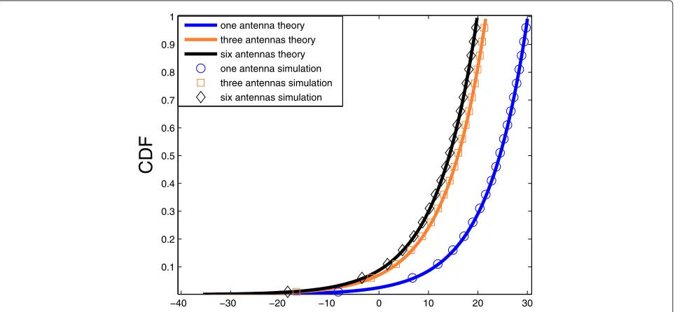
Finally, by integrating the PDFs of the transmitted and circuit consumed power over their respective ranges, we obtain the cumulative distribution functions (CDFs) for transmitted and circuit consumed power, which are shown in Figures 5 and 6, respectively. In addition, we also find the CDFs by simulation to compare them with our theoretical derivations. Moreover, as an example, we con-sider SIMO and MIMO users with three and six antennas. Furthermore, we require the users to achieve the same target SNR, ηtarget, whether SIMO or MIMO is used, in

order to make fair comparisons in terms of power expen-diture. Notice that to obtain the statistics of the overall consumed power for the SIMO case, a similar procedure is followed as the one shown for the MIMO user case. For the required values to evaluate the statistics and perform

fPmimo_diversity= ⎧

0 0.5 1 1.5 2 0.1

0.2 0.3 0.4 0.5 0.6 0.7 0.8 0.9 1

CDF

one antenna theory three antennas theory six antennas theory one antenna simulation three antennas simulation six antennas simulation

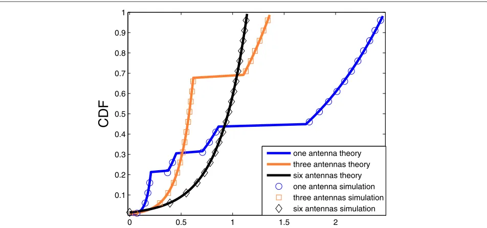
Figure 6Overall consumed power (W).User performance differences, when enhancing diversity and optimizing overall consumed power.

the simulations, we consider the values shown in Table 1. These results are discussed further in subsection 5.3.

5.2 Spatial multiplexing approach

For the following derivations, we use Shannon’s capac-ity formula for ease of analysis and without loss of generality. Thus, Equation 26 can be re-written as follows:

Tk_capacity=

J

i=1

log₂1+ηi_SC

=

J

i=1

log₂

1+Prζiσi MtN0

.

(50)

Moreover, if we assume equal gain conditions between the multiple parallel SISO channels ζi = 1,E{H2F} = MrMt = Jσi [7], Equation 50 may be re-written as:

T_{k_capacity}= J

i=1

log₂(1+ηi_SC)

=Jlog₂

1+PrMr JN0

.

(51)

Thus, by combining Equation 34 and Equation 51, we obtain the required transmitted power as:

Pt= β

Mr10

−L(_dk) 10

, (52)

Table 1 Simulation parameters

Parameter Value

MSs per macro-cell,N 20

RSs per macro-cell,R 95

Number of antennas at the receiver,Mr 6

Cell radius 150 m

Number of available RBs,X 20

Number of cells,D 1

Subcarriers per RB,ksc 12

Symbol rate per subcarrier, s 15 kbps

PTx 31.8 dBm

Pcon 23.8 dBm

PBB 11.7dBm

Maximum user transmit power 24 dBm

Shadowing, Std. Dev.,σ 3 dB

ηtarget 17 dB

Ttarget 910 kbps

εfor 17 dB SNR 4.5_symbolbits

κ 3.5

Path loss constant,a 15.3

where β =

2Tk_capacityJ −₁

JN0. To obtain the

statis-tics of the transmitted powerPt, we assume that the MSs are uniformly distributed over the cell. Moreover, from Equation 52, we obtain the inverse relationship of the path loss in function of the transmitted power.

L(Pt)= −10log10

_β

MrPt

. (53)

Thus, by using a similar approach as in Equation 39, the PDF of the transmitted power may be obtained as:

fPt =

Furthermore, we require to obtain the transmitted power in [dBm]. Thus, the inverse relationship of the transmitted power, Pt, as function of the transmitted power in [dBm],Pt_dBm, is given by:

Pt(Pt_dBm)=1e−310 Pt_dBm

10 _{. (55)}

Thereby, by using a similar approach as in Equation 45, we derive the PDF of the transmitted power in [dBm] as follows:

As in the diversity case, we should observe that in order to compute the circuit consumed powerPcirc, Equation 22,

we require the transmitted power per antenna. Thus, assuming that the transmitted power is divided evenly over all the antennas, the PDF of the transmitted power per antenna in [dBm] is:

f_P∗

Finally, we derive the inverse relationship of the trans-mitted power per antenna in [dBm] as a function of the circuit consumed power in the reverse link by combining Equations 19 and 22 as shown:

P_t∗(Pmimo_capacity)=

where γ1 = Pmimo_capacity_Mt . Moreover, by using the

trans-formation of random variables, the PDF of the circuit consumed power is shown below:

fPmimo_capacity=

where Z1 = 10log10

1e3_β

MrMt10−( a+b_log10(R)

10 )

, Z2 = A −

(0.75×PBB), andZ3=A−PBB. Finally, as in the

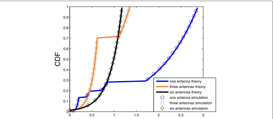
diver-sity case, by integrating the PDFs of the transmitted and circuit consumed power over their respective ranges, we obtain the CDFs for transmitted and circuit consumed power, which are shown in Figures 7 and 8, respectively. In addition, we also find the CDFs by simulation to compare them with our theoretical derivations. As an example, we consider SIMO and MIMO users carrying three and six antennas. Furthermore, we make the users independently of SIMO or MIMO to achieve the same transmission rate,Ttarget, in order to make fair comparisons in terms

of power expenditure. To evaluate the statistics and per-form the simulations, we consider the values shown in Table 1.

5.3 Analysis

From Figures 5 and 7, it is easy to see that increasing the number of antennas provides power savings at all per-centiles of the CDF when only the transmitted power is optimized. However, this trend does not remain the same when optimizing circuit power consumption. In Figure 6, in the case of diversity, we see that the SIMO curve inter-sects the MIMO curves when transmitting with three and six antennas at the 30th and 45th percentile, respectively. Moreover, for the capacity case in Figure 8, we see that the SIMO curve intersects the MIMO curves when trans-mitting with three and six antennas at the 20th and 28th percentile, respectively. This intersection point represents that in the diversity case, SIMO is more power efficient for 30% and 45% of the users in the cell when compared

to MIMO when transmitting with three and six anten-nas, respectively. The same relation holds for the spatial multiplexing case. This is because the MSs are able to experience better transmission conditions, when they are close to the BS. Thus, turning on the RF transmitter and the BB module of the relay stations is less power efficient than transmitting with only one antenna. Nevertheless, as the users get close to the cell edge increasing the num-ber of transmit antennas tends to be an energy efficient solution when circuit power consumption is optimized. This fact can be seen from Figures 6 and 8, since as the number of antennas increases, it allows the three and six antennas curves to converge faster to the tail of the distri-bution. Our analysis in this section will be useful to under-stand the performance of our framework proposed in Section 7.

6 Comparison schemes and simulation scenario To evaluate the performance of our proposal, we describe four distributed relay selection algorithms, which allow MSs and RSs to cooperate to form MIMO coalitions with the purpose of reducing the energy consumption in the reverse link. In addition, we present a baseline scheme where all MSs transmit on their own in SIMO mode. Finally, we present a centralized global optimum approach which is coordinated from the BS and based on an exhaus-tive search. For all the methods we describe, the com-munication between the MSs and RSs is made through the cooperative link. Thus, the subset of RSs willing to cooperate with the MS-n is limited by the range of the cooperative link, which naturally limits the complexity of the relay selection.

−40 −30 −20 −10 0 10 20 30

0.1 0.2 0.3 0.4 0.5 0.6 0.7 0.8 0.9 1

CDF

one antenna theory three antennas theory six antennas theory one antenna simulation three antennas simulation six antennas simulation

0 0.5 1 1.5 2 2.5 3 0

0.1 0.2 0.3 0.4 0.5 0.6 0.7 0.8 0.9 1

CDF

one antenna theory three antennas theory six antennas theory one antenna simulation three antennas simulation six antennas simulation

Figure 8User performance differences, when implementing spatial multiplexing and optimizing overall consumed power.

6.1 Minimum relaying hop (MRH) path loss selection scheme

In [37], the authors propose a relay selection method as a function of path loss. Hence, the best RS for coalition formation is the one with the least path loss to the MS, this method always chooses the RS with the most energy-efficient cooperative link.

RSc=argmin{lκnr}. (60)

From Equation 60, notice that to perform the RS selec-tion, it is just required to know the channel statistics of the cooperative link.

6.2 Best worst (BW) channel selection scheme

The BW method considers the quality of the cooperative and the reverse link of each RS. This is because both links have a direct influence on the total consumed energy to form the virtual MIMO link. In [37], the best worst chan-nel is used in which the relay whose worse chanchan-nel is the best is selected:

argmin'((((Gr, 1 lκ_nr

((

((), (61)

whereGr = hr2_F10

−L(lr)+Xσ

10 represents the channel path gain between the RS-r and the BS, and lr defines the distance between therth RS and the BS.

6.3 SM scheme

In [5], a distributed RS selection algorithm is presented which is based on the stable marriage process. This method, as in the BW channel selection scheme, requires

the channel statistics from the RSs in the reverse and cooperative link plus the channel statistics of the MSs in the reverse link. Thereby, each MS and RS are able to rank their respective candidates for coalition formation. Noticed that the SM method has the same limitation as the MRH and BW methods in the sense that each MS is only able to select one RS.

6.4 SIMO transmission

We implement a baseline scheme, where all the MSs in the network transmit in SIMO mode.

6.5 College admission framework scheme

This scheme implements our RS selection method described in Section 4.

6.6 Centralized optimum scheme

We present a centralized global optimum scheme based on an exhaustive search approach. Thus, the BS collects the required channel statistics from RSs and MSs in order to form optimal coalitions. We implement this centralized approach with the aim of finding the price of anarchy for our proposed scheme. Theprice of anarchyis computed as the difference in performance between a centralized and a distributed approach [38].

6.7 Simulation scenario

the cell area. The cell is served by an omnidirectional BS. Moreover, the system is noise limited, hence each coali-tion transmits in an independent RB to avoid co-channel interference. For the case when diversity is enhanced, we assume that all theusers(SIMO or MIMO) independent of their distance to the BS try to achieve the same target SNR,ηtarget. In the case when spatial multiplexing is used,

we assume that all the users in the network aim to achieve the same data rate,Ttarget.

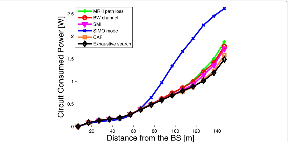
7 Results

From the simulations, we generate the CDFs and the graphs that illustrate the performance in terms ofoverall power expenditurefor the schemes presented in Section 6. When diversity is enhanced in Figure 9, we show the overall consumed power at different distances from the BS, where all the users in the cell aim to achieve the same target SNR. We observe that the distributed and cen-tralized approaches exhibit a similar performance when compared to the baseline method at close distances from the BS (up to 75 m). This is because as mentioned in the analysis presented in Section 5.1, MSs experience good transmission conditions close to the cell center. Thus, turning on the BB and the RF module of the RSs becomes less power efficient than transmitting with only one antenna. Conversely, when channel conditions are no longer so beneficial (e.g., after 75 m), we see that as the MSs move away from the BS, the increase from one to a higher number of transmit antennas allows the MS to obtain potential energy savings. Furthermore, from the

analysis shown in Section 5.1 and the results presented in Figure 9, we can confirm that, when circuit power con-sumption is optimized and spatial diversity is enhanced, by increasing the number of antennas, the obtained power savings are more visible at the cell edge than at the cell center. In Figure 10, we evaluate the system energy effi-ciency, given by Equation 28. Notice that at the 50th per-centile the CAF scheme is more energy efficient compared to the benchmark, the MRH path loss, the BW channel, and the SMI framework with improvements of 58%, 15%, 10%, and 5%, respectively. Nevertheless, the CAF scheme has losses of 10% compared to the centralized global opti-mum scheme. These losses are tolerable in practice due to the significant reductions in complexity for the CAF method compared to the centralized optimum scheme: this is discussed further at the end of this section. More-over, the better performance in energy-efficiency terms for the CAF and the centralized optimum when compared to the other distributed approaches can be easily under-stood as a direct consequence of the bigger number of antenna elements than can be involved in the coalition.

When spatial multiplexing is used, we aim to obtain gains in energy efficiency by dividing the total data rate requirements between the elements forming the virtual MIMO link. Thereby, as in the diversity case, we can see from Figure 11 that most of the power savings due to coalition formation are observed at the cell border. This is because, it is more power efficient to deliver high trans-mission rates for SIMO users close to the BS than when close to the cell edge due to the improved propagation

20 40 60 80 100 120 140 0

0.5 1 1.5 2 2.5

Distance from the BS [m]

Circuit Consumed Power [W]

MRH path loss BW channel SMI SIMO mode CAF

Exhaustive search

2 4 6 8 10 12 14

x 105 0.1

0.2 0.3 0.4 0.5 0.6 0.7 0.8 0.9 1

Energy Efficiency [kbits/J]

CDF

MRH path loss BW channel SMI SIMO mode CAF

Exhaustive search

Figure 10System CDF energy efficiency.Performance comparison when spatial diversity is implemented.

conditions. Thus, using a lower modulation order for transmitting from each antenna in a coalition when close to the cell edge becomes more power efficient than using a single transmitter. Hence, from the results obtained in Section 5.2 and Figure 11, it can be understood that increasing the number of transmit antennas to split the

total rate requirement among the transmitters by imple-menting spatial multiplexing is more power efficient in terms of overall power consumption at the cell border than at the cell center.

Finally, in Figure 12, we show the performance in terms of energy efficiency for the approaches presented

20 40 60 80 100 120 140 0

0.5 1 1.5 2 2.5

Distance from the BS [m]

Circuit Consumed Power [W]

MRH path loss BW channel SMI SIMO mode CAF

Exhaustive search

0.4 0.6 0.8 1 1.2 1.4 1.6 1.8 2 2.2 x 106 0.1

0.2 0.3 0.4 0.5 0.6 0.7 0.8 0.9 1

Energy Efficiency [kbits/J]

CDF

MRH path loss BW channel SMI SIMO mode CAF

Exhaustive search

Figure 12System energy efficiency when enhancing capacity.Performance comparison when spatial multiplexing is implemented.

in Section 6 when spatial multiplexing is implemented. We find that the centralized global optimum is 2% more energy efficient when contrasted to the CAF. Moreover, when comparing the CAF with the other distributed approaches, we see that the CAF method has improve-ments of 14%, 9%, 5%, and 91% over the MRH, the BW, the SMI, and the baseline SIMO mode, respectively. Thereby, we can confirm that increasing the number of antennas in order to use a lower modulation order results in an energy efficient solution for the network.

To conclude our comparison, the complexity of the centralized global optimum approach is compared with the proposed CAF method. On one hand, for the CAF method, each MS-n in the system has to evaluate each RS in its preferred subset of suitable candidates, Sn, by using Equation 29 or 30 depending on whether diversity or capacity are enhanced. Furthermore, each RS-r evalu-ates its preferred subsetSr of RSs by using Equation 32 or 33. Big O notation is used to describe the growth rate of the both schemes. Thus, the system performs arithmetic operations with a complexity ofO(|Sn|2)and O(|Sr|2) when candidate MSs or RS are ranked, respec-tively, where|.|is defined as the cardinality of the subset. If we assume that R N, the complexity of the can-didate ranking process is bounded by the number of RSs in the system rather than by the number of MSs. Thereby, this will allow us to upper bound the complexity of the candidate ranking byO(|Sn|2) operations. More-over, forming the MS’s preference list, ιn, Equation 31 requires a sorting operation which induces a complexity

ofO(|Sn|log(|Sn|))operations. Finally, the complexity of the decision-making, Algorithm 1 can be upper bounded by a binary search operation which requires a complex-ity of O(log(|Sn|)) operations. Therefore, the dominant factor which determines the CAF scheme complexity will be the one with the largest exponent, thus the complex-ity of the method will be upper bounded by O(|Sn|2) operations.

On the other hand, the centralized global optimum scheme is based on enumerating all possible alternatives for virtual MIMO coalition formation between the MS-n and its preferred subset of candidate RSs, Sn. This is done with the purpose of finding the optimal number of transmit antennas that would minimize the overall power consumption in the reverse link. Therefore, to guarantee that a given feasible solution is optimal, the solution should be compared with any other feasible solu-tion. In general, an exhaustive search approach, where the number of elements is discrete, is considered N P -complete [39]. A notable characteristic ofN P-complete problems is that the required time to solve the prob-lem increases very quickly as the size of the probprob-lem grows [39]. To implement the exhaustive search scheme, each MS in the system will evaluate the total num-ber of possible combinations in its preferred subset of candidate RSs, Sn. Hence, the total number of possible

combinations is computed by |Sn|

k=1

_|Sn| k

, where |Sn|

k

=

|Sn|!

k!(|Sn|−k)!. Moreover, each combination is evaluated by

20 40 60 80 100 120 140 160 10−1

100 101 102 103 104

Number of available relays

Complexity

CAF

Exhaustive search

Figure 13Complexity of the centralized optimum approach compared to the CAF method.

enhanced, respectively. Thus, this induces a complexity

of O ⎛ ⎝

|Sm|

k=1

_|Sm| k

2⎞_⎠

for the system. In addition, the

complexity of both methods (exhaustive search and CAF) increases linearly with the number of MSs in the system, N. Hence, the exhaustive search method has a complexity

ofO ⎛ ⎝N_×

|Sn|

k=1

_|Sn| k

2⎞_⎠

which is a higher order

com-plexity when compared to the comcom-plexity ofO(N× |Sn|2) for the CAF scheme. Furthermore, Figure 13 shows how the complexity of the system changes for both methods as the number of RSs increases in the system. It can be easily seen that as the number of RSs increases, the com-putational complexity of the exhaustive search increases exponentially, therefore it may not be a suitable solution to implement in real time systems.

8 Conclusions

In this paper, we considered a low complexity virtual MIMO coalition formation algorithm, which is based on game theory. The framework we proposed allows MSs to select the most suitable RSs providing the most power sav-ings in the network. Thereby, we studied energy efficient coalition formation by using the concepts of diversity and spatial multiplexing, respectively. We have shown ana-lytically and by simulation that increasing the number of transmit antennas is a more energy efficient solu-tion for users close to the cell edge rather than for

cell center users, when overall terminal power consump-tion is optimized. Furthermore, we have proven than the coalition formation algorithm we proposed is more energy efficient compared to the benchmark, the MRH path loss, the BW channel, and the SM framework with improvements of 58%, 15%, 10%, and 5% for the spatial diversity case. When implementing spatial multiplexing, the CAF method has improvements of 14%, 9%, 5%, and 91% over MRH, BW, SMI, and the baseline SIMO mode. It experiences only small performance losses of 10% and 2% when compared to an exhaustive search approach when implementing diversity and spatial multiplexing respec-tively. In addition, we presented a complexity analysis showing that the complexity of the method we proposed increases linearly as the number of RSs grows in the net-work. This is a much lower complexity when compared to the exponential growth of the exhaustive search scheme. Thus, the game-theory-based framework we proposed achieves a similar performance compared to a centralized scheme with a much lower complexity order. Hence, it may be a suitable energy-efficient solution for practical applications.

Competing interests

The authors declare that they have no competing interests.

Acknowledgements

Part of this work was done when Rodrigo Vaca was with the Institute of Digital Communications at the University of Edinburgh.

The work of Eitan Altman has been partially supported by the European Commission within the framework of the CONGAS project

Author details

1_{Scientific Division, Federal Police, 01110, Constituyentes 947, Mexico City,}

Mexico.2_{The University of Edinburgh, Institute for Digital Communications,}

King’s Buildings, Mayfield Road, EH93JL Edinburgh, UK.3INRIA, BP93, 06902 Sophia Antipolis Cedex, France.4_{Department of Electrical Engineering,}

Universidad Autónoma Metropolitana (UAM), 09340 Iztapalapa, Mexico City, Mexico.

Received: 25 November 2014 Accepted: 23 February 2015

References

1. R Vaca, J Thompson, V Ramos, Non-cooperative uplink interference protection framework for fair and energy efficient orthogonal frequency division multiple access networks. IET Commun.7(18), 2015–2025 (2013). doi:10.1049/iet-com.2013.0125

2. C Han, T Harrold, S Armour, I Krikidis, S Videv, PM Grant, H Haas, JS Thompson, I Ku, C-X Wang, TA Le, MR Nakhai, J Zhang, L Hanzo, Green radio: radio techniques to enable energy-efficient wireless networks. IEEE Commun. Mag.49(6), 46–54 (2011).

doi:10.1109/MCOM.2011.5783984

3. AR Jensen, M Lauridsen, P Mogensen, TB Sørensen, P Jensen, in

Proceedings of the IEEE 76th Vehicular Technology Conference (VTC-Fall). LTE

UE power consumption model for system level energy and performance optimization (IEEE, Quebec City, Canada, 2012), pp. 1–6.

doi:10.1109/VTCFall.2012.6399281

4. R Vaca, J Thompson, V Ramos, inProceedings of the IEEE 76th Vehicular

Technology Conference (VTC-Fall). Uplink interference protection as a

non-cooperative game over OFDMA networks (IEEE, Quebec City, Canada, 2012), pp. 1–5. doi:10.1109/VTCFall.2012.6399092

5. R Vaca, E Altman, J Thompson, V Ramos, inProceedings of the 24th Annual IEEE International Symposium on Personal Indoor and Mobile Radio

Communications (PIMRC). A stable marriage framework for distributed

virtual MIMO coalition formation (IEEE, London, UK, 2013), pp. 2722–2727. doi:10.1109/PIMRC.2013.6666606

6. R Vaca, J Thompson, E Altman, V Ramos, inProceedings of the IEEE INFOCOM Workshop on Green Cognitive Communications and Computing

Networks. A game theory framework for a distributed and energy efficient

bandwidth expansion process (IEEE, Toronto, Canada, 2014), pp. 712–717. doi:10.1109/INFCOMW.2014.6849318

7. A Paulraj, R Nabar, D Gore,Introduction to Space Time Wireless

Communications. (Cambridge University Press, Cambridge UK, 2003)

8. J Jiang, M Dianati, M Imran, Y Chen, inProceedings of the IEEE 76th

Vehicular Technology Conference (VTC-Fall). Energy efficiency and optimal

power allocation in virtual-MIMO systems (IEEE Quebec City, Canada, 2012), pp. 1–6. doi:10.1109/VTCFall.2012.6399002

9. S Sesia, I Toufik, M Bake,LTE-the UMTS Long Term Evolution from Theory to

Practice. (Wiley, Chichester, USA, 2009)

10. Z Han, D Niyato, T Ba¸sar, A Hjørungnes,Game Theory in Wireless and

Communication Networks. (Cambridge University Press, Cambridge, UK,

2012)

11. G Quer, F Librino, L Canzian, L Badia, M Zorzi, Inter-network cooperation exploiting game theory and bayesian networks. IEEE Trans. Commun.61(10), 4310–4321 (2013).

doi:10.1109/TCOMM.2013.082813.120710

12. S Hussain, A Azim, J Park, Energy efficient virtual MIMO communication for wireless sensor networks. Telecommun. Syst.42(1–2), 139–149 (2009). doi:10.1007/s11235-009-9176-7

13. W Saad, Z Han, M Debbah, A Hjorungnes, T Ba¸sar, Coalitional game theory for communication networks. IEEE Signal Process. Mag.26(5), 77–97 (2009). doi:10.1109/MSP.2009.000000

14. F Pantisano, M Bennis, W Saad, R Verdone, M Latva-aho, inProceedings of

the IEEE Wireless Communications and Networking Conference (WCNC).

Coalition formation games for femtocell interference management: a recursive core approach (IEEE, Cancun, Mexico, 2011), pp. 1161–1166. doi:10.1109/WCNC.2011.5779295

15. AS Ibrahim, AK Sadek, W Su, KJR Liu, Cooperative communications with relay-selection: when to cooperate and whom to cooperate with? IEEE Trans. Wireless Commun.7(7), 2814–2827 (2008).

doi:10.1109/TWC.2008.070176

16. EG Larsson, EA Jorswieck, Competition versus cooperation on the MISO interference channel. IEEE J. Selected Areas Commun.26(7), 1059–1069 (2008). doi:10.1109/JSAC.2008.080904

17. K Yazdi, E Gammal, P Schitner, inAllerton Conference on Communications,

Control and Computing. On the design of cooperative transmission

schemes, (2003)

18. N Jindal, U Mitra, A Goldsmith, inInternational Symposium on Information

Theory (ISIT). Capacity of ad-hoc networks with node cooperation (IEEE,

2004), p. 269. doi:10.1109/ISIT.2004.1365306

19. S Cui, A Goldsmith, A Bahai, Energy efficiency of MIMO and cooperative MIMO techniques in sensor networks. IEEE J. Selected Areas Commun.

22(6), 1089–1098 (2004). doi:10.1109/JSAC.2004.830916

20. Z Han, D Niyato, W Saad, T Ba¸sar, A Hjørungnes,Game Theory in Wireless

and Communication Networks. (Cambridge University Press, Cambridge,

UK, 2012)

21. Z Han, R Liu, Fair multiuser channel allocation for OFDMA networks using Nash bargaining solutions and coalitions. IEEE Trans. Commun.53(8), 1366–1376 (2005). doi:10.1109/TCOMM.2005.852826

22. W Saad, Z Han, M Debbah, A distributed coalition formation framework for fair user cooperation in wireless networks. IEEE Trans. Wireless Commun.8(9), 4580–4593 (2009). doi:10.1109/TWC.2009.080522

23. H Burchardt, S Sinanovic, Z Bharucha, H Haas, Distributed and autonomous resource and power allocation for wireless networks. IEEE Trans. Commun.61(7), 2758–2771 (2013).

doi:10.1109/TCOMM.2013.053013.120916

24. WA Prasetyo, H Lu, H Nikookar, inProceedings of the 41st European

Microwave Conference (EuMC). Optimal relay selection and power

allocation using game theory for cooperative wireless networks with interference. IEEE (IEEE, Manchester, UK, 2011), pp. 37–40

25. S Fujio, D Kimura, inProceedings of the IEEE 24th International

Symposium on Personal Indoor and Mobile Radio Communications (PIMRC).

Energy saving effect of solar powered repeaters for cellular mobile systems. IEEE (IEEE London, UK, 2013), pp. 2841–2845.

doi:10.1109/PIMRC.2013.6666631

26. J Laneman, D Tse, G Wornell, Cooperative diversity in wireless networks: efficient protocols and outage behavior. IEEE Trans. Inf. Theory.50(12), 3062–3080 (2004). doi:10.1109/TIT.2004.838089

27. H Burchardt, Z Bharucha, G Auer, H Haas, Uplink interference protection and scheduling for energy efficient OFDMA networks. EURASIP J. Wireless Commun. Netw.2012(180) (2012). doi:10.1186/1687-1499-2012-180

28. H Dai, inProceedings of the IEEE International Conference on Acoustics,

Speech and Signal Processing (ICASSP). Distributed versus co-located MIMO

systems with correlated fading and shadowing, vol. 4 (IEEE, Toulouse, France, 2006), pp. 561–564. doi:10.1109/ICASSP.2006.1661030

29. Q Li, G Li, W Lee, M-I Lee, D Mazzarese, B Clerckx, Z Li, MIMO techniques in WiMAX and LTE: a feature overview. IEEE Commun. Mag.48(5), 86–92 (2010). doi:10.1109/MCOM.2010.5458368

30. T Cover, J Thomas,Elements of Information Theory. (Wiley-Interscience, Hoboken, NJ, USA, 1991)

31. K Bobae, K Cholho, L Jongsoo, A dual-mode power amplifier with on-chip switch bias control circuits for LTE handsets. IEEE Trans. Circuits Syst.

58(12), 857–861 (2011). doi:10.1109/TCSII.2011.2172528

32. D Gale, M Sotomayor, Some remarks on the stable matching problem. Discrete Appl. Math.11(3), 223–232 (1985).

doi:10.1016/0166-218X(85)90074-5

33. A Roth, E Peranson, The redesign of the matching market for American physicians: some engineering aspects of economic design. Am. Econ. Rev.89(4), 748–780 (1999). doi:10.1257/aer.89.4.748

34. K Iwama, S Miyazaki, inProceedings of the International Conference on

Informatics Research for Development of Knowledge Society Infrastructure. A

survey of the stable marriage problem and its variants (IEEE, Kyoto, Japan, 2008), pp. 131–136. doi:10.1109/ICKS.2008.7

35. S Sanayei, A Nosratinia, Antenna selection in MIMO systems. IEEE Commun. Mag.42(10), 68–73 (2004). doi:10.1109/MCOM.2004.1341263 36. D Gale, LS Shapley, College admissions and the stability of marriage. Am.

Math. Mon.69(1), 9–15 (1962)

37. V Sreng, H Yanikomeroglu, D Falconer, inProceedings of the IEEE 58th

cellular networks with peer-to-peer relaying (IEEE, 2003), pp. 1949–1953. doi:10.1109/VETECF.2003.1285365

38. EG Larsson, EA Jorswieck, J Lindblom, R Mochaourab, Game theory and the flat-fading gaussian interference channel. IEEE Signal Process. Mag.

26(5), 18–27 (2009). doi:10.1109/MSP.2009.933370

39. Z Han, KJR Liu,Resource Allocation for Wireless Networks. (Cambridge University Press, Cambridge, UK, 2008)

Submit your manuscript to a

journal and benefi t from:

7Convenient online submission 7Rigorous peer review

7Immediate publication on acceptance 7Open access: articles freely available online 7High visibility within the fi eld

7Retaining the copyright to your article