Bayesian Methods for Quantitative Trait Loci Mapping Based on Model
Selection: Approximate Analysis Using the Bayesian Information Criterion
Roderick D. Ball
New Zealand Forest Research Institute, Rotorua 3201, New Zealand
Manuscript received April 13, 2000 Accepted for publication August 30, 2001
ABSTRACT
We describe an approximate method for the analysis of quantitative trait loci (QTL) based on model selection from multiple regression models with trait values regressed on marker genotypes, using a modifi-cation of the easily calculated Bayesian information criterion to estimate the posterior probability of models with various subsets of markers as variables. The BIC-␦criterion, with the parameter␦increasing the penalty for additional variables in a model, is further modified to incorporate prior information, and missing values are handled by multiple imputation. Marginal probabilities for model sizes are calculated, and the posterior probability of nonzero model size is interpreted as the posterior probability of existence of a QTL linked to one or more markers. The method is demonstrated on analysis of associations between wood density and markers on two linkage groups inPinus radiata.Selection bias, which is the bias that results from using the same data to both select the variables in a model and estimate the coefficients, is shown to be a problem for commonly used non-Bayesian methods for QTL mapping, which do not average over alternative possible models that are consistent with the data.
Q
UANTITATIVE trait loci (QTL) mapping is the or ANOVA) or at each of a series of points on the genome (interval mapping;LanderandBotstein1989). process of finding and estimating associationsbe-tween a continuous quantitative trait and a set of DNA An alternative to interval mapping, also involving multi-ple hypothesis tests, is based on regression on flanking markers that have been previously placed on a genetic
map, with the ultimate goal of determining the genetic markers (HaleyandKnott1992). SeePaterson(1995) andDoerge et al.(1997) for reviews.
architecture of a trait, or finding markers that can be
Markers or loci where the test statistic exceeds a used to select for preferred values of the trait. The
threshold are chosen and considered to be “detected.” map is generally assumed to be known and correct and
Problems with these methods are that QTL are often should cover a significant proportion of the genome.
detected but where an independent verification popula-QTL mapping works on the principle that if a locus
tion is used the markers are subsequently not verified (called a QTL) on the genome is causing variation in
and/or the estimated effects are much smaller in the a trait, and data are obtained from a cross (or pedigree)
verification population (see,e.g.,Beavis1994;Wilcox
in which the QTL is segregating, then values of the trait
et al.1997;Melchingeret al.1998). The latter problem
will be correlated with markers linked to that locus.
is an example of selection bias, which is well known to The closer the marker, the closer the correlation. For
statisticians in the context of stepwise regression (Miller
a marker at a given distance from the QTL, the larger
1990). Selection bias occurs when the same data are the effect of the QTL, the larger the effect of the marker,
used to both select the variables in a regression model as can be estimated from differences between subsets
and to estimate the coefficients. of the population with different marker classes. The
Bayesian statistics:Bayesian statistics aim to compute statistical problem is to estimate the effects and locations
probability distributions for the underlying parameters of QTL or the effects of using associated markers to
in a model. With this information it is, in principle, select progeny. The problem is challenging statistically
possible to compute probabilities of any events or quan-because one or more QTL for a trait could be located
tities of interest such as the probability of a linked QTL anywhere on the genome.
in a region or the expected gain from marker-aided Non-Bayesian QTL mapping:A common approach is
selection. to carry out a hypothesis test at each marker (at-test
An important aspect of Bayesian analysis is the use of
marginal distributions. In the method of this article, the
probability distributions of estimates and predictions
Address for correspondence:New Zealand Forest Research Institute,
are averaged over the values of parameters in the model P.B. 3020, Rotorua 3201, New Zealand.
E-mail: [email protected] and over possible models, rather than with parameters
set to their most likely values in the most likely model, OVERVIEW: BAYESIAN QTL MAPPING USING MODEL SELECTION
as is usually the case in non-Bayesian methods, such as
maximum likelihood. In a single model, estimates and Our approach is to relate trait values directly to confidence intervals from maximum likelihood will be marker genotypes, using multiple linear regression. similar to their Bayesian counterparts provided the sam- Since there are many markers in a typical cross, most ple size is large enough. More significant differences of these will not be near to a QTL. Therefore it is arise, however, when testing “precise hypotheses” (Ber- necessary to choose a model or models with subsets of gerandBerry1988). Existence or nonexistence of a markers selected.Broman(1997) advocated a stepwise QTL linked to a particular marker is one example. This regression approach for choosing the “best” model. difference occurs because Bayesian inference considers However, we shall see that particularly with small sample the probability of the data under each of the two possible sizes there can be a multiplicity of models that are com-models,e.g.,H0: ⫽0 andH1: ⬆0. The non-Bayesian patible with the data, and these alternative models need hypothesis test considers the tail probability for a test to be considered along with their probabilities ( Raf-statistic underH0, which can be shown to be approxi- tery1995,Rafteryet al.1997).
mately equivalent to a tail probability of the posterior Our strategy is to build on methods for model se-distribution for the parameter,, being testedunder H1. lection in linear models from the statistical literature, This does not allow for the finite nonzeroprior probability starting with the Bayesian information criterion (BIC;
(it must be nonzero or we would not need to test it) Schwartz1978) in this article, and a modification of thatH0is true. More generally,where multiple models are the Bayesian method for model selection inhierarchical
consistent with the data, it is necessary to consider all these linear models(a whole family of linear models combined
models according to their probabilities for valid statistical infer- in an overarching single model) ofGeorgeand
McCul-ence(cf.Raftery1995,Rafteryet al.1997). loch (1993) in future work. Our methodology is to
Bayesian QTL mapping: A number of articles on the full Bayesian approach as the regression method of Bayesian approaches to QTL mapping have appeared Haley and Knott (1992) is to interval mapping—a (reviewed byHoescheleet al.1997). simpler more easily calculated method that nevertheless Several more recent articles have appeared that simul- captures (at least approximately) the important aspects taneously consider multiple models with different num- of the full Bayesian analysis,i.e., the posterior probability bers of QTL (SatagopanandYandell1996;Satago- that a QTL is located in a given region, or the marginal
panet al.1996;Heath1997;Sillanpa¨a¨andArjas1998, distribution for the size of effects.
1999;StephensandFisch1998). These articles use the There is a major difference between our approach “reversible jump” methodology of Green (1995) for and others that consider multiple models. Previous ap-constructing a sampler that jumps between models of proaches consider the model as specifying only the num-different dimension. A major challenge remains to ob- ber of QTL on each linkage group, while the locations tain a rapidly converging sampler for the full Bayesian of the QTL are parameters in the model. In our ap-model (D. A. Stephens,personal communication). The proach the QTL are at fixed locations. In other words methods are complex to program and as yet there is a QTL in our model really is a quantitative traitlocus.
no publicly available program with demonstrated rapid A QTL at a different position is considered a different
convergence. QTL and is represented by a different model. This
in-More easily implemented and faster methods are use- creases the number of models but simplifies the analysis ful, for people without access to the above programs, of a given model.
bias that results when the effects of markers and the tively genotyped data, where individuals genotyped are selected from the tails of the trait distribution. effects of allelic substitution are estimated conditional
on selection. Further discussion of selection bias is given
Two linkage groups (linkage groups 1 and 3) were below and a small simulation study demonstrating the
chosen for illustration of our method. Linkage group effect of model averaging on selection bias is given in
3 was chosen because it contained statistically significant theappendix.
associations found from previous (non-Bayesian) analy-In this article approximate posterior probabilities for
ses (Kumar et al. 2000). Linkage group 1 was chosen models are obtained using a modification of the easily
as simply another linkage group where no significant calculated BIC (Schwartz1978). The probabilities are
association had previously been found. approximate but good enough to give a rough
indica-A non-Bayesian analysis is given for comparison. This tion. Moreover, it may be possible, by adjusting a single
is based on t-tests for the regression coefficient of a parameter, to fine tune the method. We apply the
marker in a single-marker model for the trait and re-method to QTL mapping data for wood density inPinus
peated for each available marker. Missing data were
radiataand demonstrate the need to consider multiple
removed (rather than using multiple imputation) be-models in assessing the probability of existence of a
fore testing each marker. Genome-wise thresholds for QTL and obtaining estimates of the effects of allelic
thet-statistics were estimated using a permutation test substitution at a marker free of selection bias.
(cf.ChurchillandDoerge1994).
Bayesian information criterion:Approximate probabili-ties for models can be obtained from the BIC, given by DATA AND METHODS
BIC⫽ nlog(1⫺ R2)⫹klog(n), (1)
The method is demonstrated on analysis of
associa-tions between wood density and markers from two link- wherekis the number of parameters fitted in the model, age groups inP. radiata. nis the number of observations, andR2is the proportion
Marker and trait data were obtained from a single of variance explained by the model.Schwartz(1978) full-sib family with parents 850.55 and 850.96, for the showed that with no prior (all modelsa priori equally purpose of QTL detection. likely), the posterior probability (p) of a model is
ap-Trait data:Two 5-mm pith-to-bark cores were taken proximately proportional to from each tree. Usable data were available from 93 trees.
p⬀exp(⫺BIC/2). (2)
Wood density was assessed from each of the cores by X-ray densitometry (Cown and Clement 1983). The
This approach has the advantage of relative simplicity traits considered here were juvenile wood density at
and consequent ease of computation. It has the disad-ages 1–5 years (estimated as the area weighted average
vantage that the relationship (2) between BIC and prob-of rings 1–5) as the average outerwood density
(esti-abilities of models is asymptotic; i.e., it relies on large mated as the average density of the outer 5 cm from
sample sizes. To allow for thisBroman(1997) advocates each core), adjusted for site and replicate differences,
a modification, BIC-␦, and standardized. These traits are similar to the traits
WD1_5, WD14 (outerwood density, not standardized) BIC-␦ ⫽nlog(1⫺ R2)⫹k␦log(n), (3)
analyzed byKumaret al.(2000).
where ␦ is a constant. Broman recommends␦ ⫽ 2 or Marker data:There were 126 markers of various types
␦ ⫽3; however, the best value to use depends on sample [randomly amplified polymorphic DNA (RAPD),
ampli-size and other factors and is a topic for future research. fied fragment length polymorphism (AFLP), and simple
To handle missing values, multiple imputation (Rubin
sequence repeat (SSR)] in 23 linkage groups with from
and Schenker 1986) was used to generate multiple 2 to 16 markers per linkage group, which were
segregat-instances of the data sets with missing markers randomly ing in pseudobackcross configuration, for the 850.55
estimated according to the values and proximity of parent. There were 1171 missing marker values (10%
flanking markers. This is an alternative to the Haley
of the marker data). These values were due to indistinct
andKnott(1992) method of assigning a weighted aver-bands or PCR failure and are assumed missing at
ran-age of flanking marker values to the missing markers. dom. All 93 trees had one or more missing marker
The multiple imputation approach allows for uncer-values. For further information on the study seeKumar
tainty in the imputed values.
et al.(2000).
Ten imputations were used. Rubin and Schenker re-Note that
port good results with 2–3 imputations for estimating means and confidence intervals for continuous random 1. with markers in pseudobackcross configuration, the
analysis is equivalent to the analysis of a backcross, variables. However, since we apply imputation to marker values that take on discrete values (0 or 1) we may need and
selec-lelic substitution for outerwood density at markers We now modify the probabilities of (2) by considering the prior probability for a QTL to be present at a given RAPD.192 and A47.c were reestimated for each of the
10 imputations separately. locus. If there are k QTL present, and markers are spaced on average at s cM in a genome of length L
Rather than repeating model fits for each imputation,
the data from each imputation were combined, giving cM, then the probability that a QTL is present in the immediate neighborhood of a marker is
a data set with n ⫻ nI points, where nI denotes the number of imputations used. The multiple imputation
estimate of BIC is given by applying (1), with n being ≈1⫺
冢
1⫺ sL
冣
k
. (4)
the number of observations in the original (unimputed) data and R2 the value ofR2 from the model fitted to
Our markers are spaced atⵑ12–15 cM on a genome the combined data set. This can be justified by consider- of estimated length 2000 cM (Wilcox1997). A genetic ing the likelihood function for an analysis with each of architecture with many small QTL seems likely since thenIimputations of an observation given weight 1/nI; large effect QTL should have been detected by previous
i.e., the likelihood contribution for all imputations of a studies (Wilcox et al. 1997). If there are 20 QTL we data point is the same as the likelihood contribution havek⫽20, s⫽ 12,L ⫽2000 cM, giving ≈0.1. To for the data point in the unimputed data set, if there show sensitivity to, and to accommodate readers who is no missing marker, and the average of the likelihood believe there are fewer QTL likely to be present, we contributions from the various imputations if there is a also calculate posterior probabilities for model size for
missing marker. ⫽0.03 or 0.06 corresponding to 5 or 10 QTL,
respec-Calculations for this work used Splus version 3.4 for tively, in the analysis below.
Unix (Beckeret al.1988). The Splus function bicreg.qtl, Ideally one would like to have a marker at each QTL a modification of the function bicreg (Raftery1995), location. What we can guarantee is a marker at each was used to search through possible models and calcu- QTL locationto within the resolution of the marker linkage late the BIC criterion and associated quantities. The map.So for each QTL configuration, the “true” model search procedure used by bicreg is essentially an exhaus- (our best approximation) will be a model such that each tive search using the all subsets regression function marker is selected (in the model) if and only if it is the leaps, returning the value ofR2, for each model, from
closest marker to some QTL or, equivalently, there is a which BIC is calculated. Backward elimination is used QTL in the region around a marker extending halfway to reduce the number of variables to the limit of 30 prior to each of the adjacent flanking markers. QTL are as-to calling leaps. Our function contains modifications as-to sumed to occur randomly in any s-cM interval, with allow for adjustment for multiple imputations, prior occurrences in various intervals being mutually inde-distributions, and the parameter␦. The function bicreg pendent. So the prior probability that each marker is gives estimates of average effects for variableconditional selected is, and the events of selection or nonselection
on selection(i.e., averaged over models in which the vari- of the various markers area priorimutually independent.
able is selected). We also give unconditional estimates, The prior probability that a given model withkmarkers where the effect of a variable (marker effect) is defined selected is the true model is therefore
to be zero in models where the marker is not selected,
and model-averaged effects of allelic substitution (i.e., k(1 ⫺ )(n⫺k). (5)
estimates of the difference between marker classes).
The combined prior probability for all models with k
Several options from bicreg can be adjusted to control
markers linked to QTL is therefore the binomial proba-the amount of computing done. These are Occam’s
bility razor constant OR and the lower limit on number of
models nbest considered for each model size. Initially q!
(q⫺ k)!k!
k(1⫺ )(q⫺k), (6)
at least nbest models of each size are considered, then models less likely than the most likely model by the
factor OR or more are eliminated from consideration. where qis the total number or markers being consid-ered.
The calculations for Tables 2–4 all used OR ⫽ 10,000
and nbest⫽100. In calculating the posterior probability of a model
the estimate from (2) is multiplied by the probability Incorporating prior probabilities:The BIC criterion
does not incorporate prior information. For any given from (5).
Marginal probabilities of QTL location:The marginal prior, the effect of the prior will be negligible for a
sufficiently large sample size. For BIC-␦increasing␦may probability that a QTL is in a region is estimated as the marginal probability that one or more of the markers compensate for a lower prior probability of linkage. We
prefer, however, to explicitly incorporate the prior and in the region are selected, which is obtained from the BIC calculation by summing posterior probabilities for leave the parameter ␦ to compensate for the effects
stitution:Letmdenote the number of markers andnthe where the marker is not selected) of the marker effect for markerigiven by
number of progeny. We consider all possible models, corresponding to all 2mpossible subsets of markers. Each
bˆi,av⫽
兺
kpkbˆi,k. (10)
model is characterized by a set of markers that are
se-lected.Let Mkdenote the kth model, letpkdenote the
Similarly, let dˆi,avbe the model-averaged estimate of posterior probability ofMk, letMk(i)denote the model
allelic substitution for theith marker given by where only markeri is selected, and let Sidenote the
set of models with markeriselected.
dˆi,av⫽
兺
kpkdˆi,k. (11)
Let Mj be the jth marker, with alleles labeled 1 and 2, and yi and Mj(i)the trait value and value of the jth
Selection bias:Selection bias is a well-known phenom-marker for the ith individual, respectively. Let V(Mj)
enon that occurs when using a model selection method,
(thevicinityof markerj), be defined as the set of points
such as stepwise regression, to select the variables in a closer to markerjthan to any other marker.
model, and the same data used for model selection are The models fitted are of the form
used to estimate the effects. Conditional on selection, the estimates of effects are greater in absolute value than
yi⫽
兺
m
j⫽1
bj,kxij⫹ eij, i⫽1, . . . ,n, (7)
the true values, because in the sampling distribution of effects, the values larger than some threshold are where
selected. An implicit model selection step is being car-ried out when selecting markers using the conventional
xij ⫽
⫹1/2 ifMj(i)⫽2
⫺1/2 ifMj(i)⫽1,
(8)
t-test or interval mapping methods.
Our estimate of selection bias is obtained by compar-and the errorseijare assumed to be normally distributed. ing the model-averaged estimates, which we argue have
Effects of markers: The regression coefficients for Mk no problem with selection bias (cf.appendix), to
corre-are denoted bybj,kor simply bjwhen there is no need sponding estimates conditional on selection, i.e., esti-to distinguish models. We refer esti-tobj,kasthe effect of the mates averaged over models in which the marker is
jth marker inMk. The coefficientsbj,kfor unselected mark- selected.
ers are set to zero by convention, so that the sum in (7) Selection bias in the effect of allelic substitution is is effectively over selected markers. estimated as
Effects of allelic substitution:The effect of allelic
substitu-tion, di,k, for Mi in Mkis defined as the difference in
selection bias≈dˆi,k(i)⫺dˆi,av
dˆi,av
(12) population means between the two marker classes ifMk
is the true model.
and is given to indicate the bias likely to result from Note that
commonly used methods that both select a marker or 1. the effect of allelic substitution di,k(i) in the model markers on the basis of some test (effectively selecting
Mk(i)where only markeriis selected and is the same a model) and estimate the effect of the marker using
as the conventional effect of allelic substitution, and the same data. The actual selection bias when using the 2. the effects of allelic substitutiondi,kare not the same non-Bayesian methods depends on the threshold used as the effects of markers bi,k, except in the model for the test statistic (it is higher with higher threshold
Mk(i), in which case or lowerPvalue).
The concepts of this selection and their
interpreta-bi,k(i)⫽di,k(i)
tions are summarized in Table 1. Further discussion of and the observed difference between the averages selection bias and a small simulation study are given in of marker classes is an unbiased estimate of both the
appendix, showing the selection bias in thet-test quantities.
method, that Bayesian estimates have negative bias (shrink-age toward zero), in the case of model uncertainty, and
Estimation:Letbˆi,k,dˆi,kbe the conventional
maximum-that even conditional on selection using the t-test at likelihood estimates of estimates ofbi,k,di,k, respectively,
quite low thresholds, the model-averaged estimates did in modelMk.
not show selection bias. Let bˆi,s be the estimated effect for the ith marker
conditional on selection (i.e., the effect, averaged over models, in which the marker is selected) given by
RESULTS
bˆi,s⫽
RMk僆Sipkbˆi,k
RMk僆Sipk
, (9) Results are given for␦ ⫽1, 1.5, 2, and 3. For simplicity of discussion, unless otherwise stated, all comments be-low refer to the case ␦ ⫽ 1. Higher values are more and let bˆi,av, be the unconditional estimate (averaged
TABLE 1
Notation, terminology, and interpretations for models, effects of markers, effects of allelic substitution, and associated estimates
Symbol Concept Practical interpretation
Mi ith marker
V(Mi) Vicinity ofith marker Region closer toith marker than any other
Mk kth model
pk Posterior probability ofMk
— Marginal probability of selection of Probability of existence of one or more QTL in
markers(s) in a region the region
bˆi,s Estimated effect of markerMicondi- Estimate of QTL effect assuming QTL exists in
tional on selection V(Mi)
bˆi,av Unconditional (i.e., model averaged) Posterior expected gain from QTL inV(Mi) effect ofMi
dˆi,k(i) Conditional effect of allelic substitution Estimated gain from selection on Mi assuming QTL exists only inV(Mi)
dˆi,av Unconditional (i.e., model averaged) Posterior expected gain if using Mifor marker-effect of allelic substitution aided selection
on a linkage group, larger amounts of selection bias, probabilities for a QTL;e.g., with␦ ⫽2, 3 the probability that a QTL is present on linkage group 3 is 0.97, 0.76, and smaller estimates of effects of allelic substitution.
Table 2 shows the marginal probabilities for models respectively. Evidence for a QTL, albeit not strong, per-sists to␦ ⫽3.
of various sizes for two linkage groups, linkage groups
1 and 3. These probabilities are obtained by amalgamat- For outerwood, from Table 2 with␦ ⫽1, the probabil-ity that a QTL is present on linkage groups 1, 3 is 0.38, ing probabilities of all models of each given size.
The marginal probability that one or more QTL are 0.88, respectively. On linkage group 3 the probability of model size 2 was 0.28, indicating the possibility of present on a linkage group is the probability that the
model size is 1 or more or 1 minus the probability that two QTL separated by one or more markers. With␦ ⱖ 2 the probability that a QTL is present is⬍0.5 on each the model size is zero.
For juvenile wood, from Table 2 with ␦ ⫽ 1, the linkage group.
Marginal probabilities for model size for various val-probability that a QTL is present on linkage groups 1,
3 is 0.17, 0.997, respectively. On linkage group 3 the ues of the prior probability ⫽0.03, 0.06, 0.1, corre-sponding to a prior expectation of 5, 10, 20 QTL, respec-probability of model size 2 was 0.26, indicating the
possi-bility of two QTL separated by one or more markers. tively, are shown in Table 3.
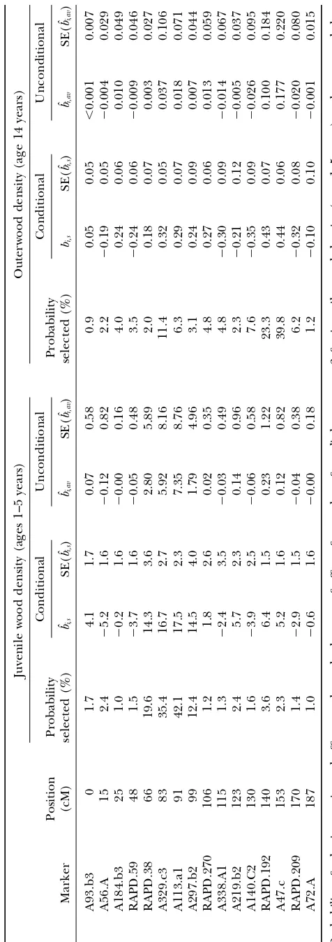
Table 4 shows the probability of selection, estimated Higher values of ␦are more conservative, giving lower
TABLE 2
Marginal probabilities for model size estimated using the BIC-␦criterion for various values of␦
Linkage group 1 Linkage group 3
k ␦ ⫽1 ␦ ⫽1.5 ␦ ⫽2 ␦ ⫽3 ␦ ⫽1 ␦ ⫽1.5 ␦ ⫽2 ␦ ⫽3
Juvenile wood density (ages 1–5 years)
0 0.832 0.940 0.979 0.998 0.003 0.010 0.033 0.240
1 0.155 0.058 0.020 0.002 0.710 0.877 0.928 0.757
2 0.013 0.002 ⬍0.001 ⬍0.001 0.263 0.109 0.038 0.003
3 ⬍0.001 ⬍0.001 ⬍0.001 ⬍0.001 0.024 0.003 ⬍0.001 ⬍0.001
Outerwood density (age 14 years)
0 0.618 0.840 0.943 0.994 0.123 0.369 0.668 0.953
1 0.359 0.157 0.057 0.006 0.562 0.542 0.316 0.047
2 0.022 0.003 ⬍0.001 ⬍0.001 0.275 0.085 0.016 ⬍0.001
3 ⬍0.001 ⬍0.001 ⬍0.001 ⬍0.001 0.038 0.004 ⬍0.001 ⬍0.001 4 ⬍0.001 ⬍0.001 ⬍0.001 ⬍0.001 0.003 ⬍0.001 ⬍0.001 ⬍0.001
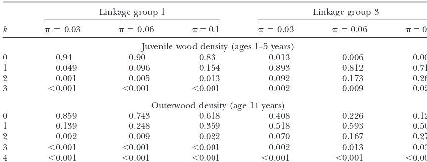
TABLE 3
Marginal probabilities for model size estimated using the BIC-␦criterion for various prior probabilities of selection of markers
Linkage group 1 Linkage group 3
k ⫽0.03 ⫽0.06 ⫽0.1 ⫽0.03 ⫽0.06 ⫽0.1
Juvenile wood density (ages 1–5 years)
0 0.94 0.90 0.83 0.013 0.006 0.003
1 0.049 0.096 0.154 0.893 0.812 0.710
2 0.001 0.005 0.013 0.092 0.173 0.263
3 ⬍0.001 ⬍0.001 ⬍0.001 0.002 0.009 0.024
Outerwood density (age 14 years)
0 0.859 0.743 0.618 0.408 0.226 0.123
1 0.139 0.248 0.359 0.518 0.593 0.562
2 0.002 0.009 0.022 0.070 0.167 0.274
3 ⬍0.001 ⬍0.001 ⬍0.001 0.002 0.013 0.038
4 ⬍0.001 ⬍0.001 ⬍0.001 ⬍0.001 ⬍0.001 ⬍0.001
Marginal probabilities for model size (k) for linkage groups 1 and 3, for juvenile wood density (ages 1–5 years), and outerwood density (age 14 years). Probabilities were estimated using BIC-␦, with␦ ⫽1, and a prior probability of ⫽0.03, 0.06, and 0.1 for each marker to be in the model, corresponding to 5, 10, and 20 QTL, respectively.
effects, and standard errors for markers, obtained by nome-wiseP⬍0.01) and markers A329.c3 and A297.b2 had comparison-wisePvalues ofⵑ0.0001 (genome-wise combining effects across models according to their
probabilities. Effects (bˆi,s) are shown conditional on se- P⬍0.05).
For outerwood density, RAPD.192 and A47.c have lection (averaged over models, in which the marker is
selected, corresponding to estimated QTL effects assum- comparison-wiseP values ofⵑ0.002.
Note the selection bias of 27, 25, and 75% for the ing a QTL is present) or unconditionally (bˆi,av, averaged
over all models with the effect set to zero in models three largest effect markers for juvenile wood density and 85 and 77% for the two largest effect markers. If where the marker is not selected, corresponding to the
posterior mean of estimated QTL effects for QTL in higher values of␦are used these estimates will increase. The calculations for outerwood density for linkage the vicinity of markeri).
Note that no single marker has a high posterior proba- group 3 with 16 markers took ⵑ9 min in Splus on a Silicon Graphics Indigo Impact 10,000 running Irix 6.2, bility. This reflects uncertainty in the positional location
of a QTL. For example, for juvenile wood density the finding probabilities for a total of 332 models.
Calculations of just the model probabilities in Table markers RAPD.38 to A297.b2 had probabilities of 12–
42%. Outside this region posterior probabilities dropped 2 with ␦ ⫽1 and nbest ⫽10 took 6 sec.
The effects of allelic substitution for outerwood den-off to low values. This suggests that a QTL if present is
most likely to be in the region between these two mark- sity at markers RAPD.192 and A47.c were reestimated for each of the 10 imputations separately. The standard ers or possibly in the closer one-half of the adjoining
intervals beyond this region. The marginal probability deviation between imputations was 0.075, giving a stan-dard error of the mean for 10 imputations ofⵑ0.02, that a QTL is in this region is estimated at 0.995 and
contains practically all of the posterior probability of which is acceptable. models of nonzero size.
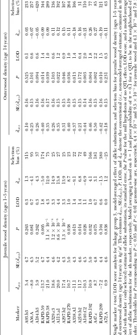
Table 5 gives the conventionalt-test/LOD score
anal-DISCUSSION ysis one marker at a time for linkage group 3 plus
model-averaged estimates of the effect of allelic substitution The BIC method with multiple imputations for miss-ing values gives estimates of posterior probabilities that and estimates of selection bias in the
non-model-aver-aged estimates of allelic substitution. The conventional can be easily and rapidly calculated for a linkage group. With 10 imputations the standard error of the mean of estimate of allelic substitutiondˆi,k(i)for the ith marker
is subject to selection bias—it was obtained from the the effects of allelic substitution estimated separately for each imputation was only about one-eighth of the same data that were used to select the marker. The
model averaged estimate dˆi,av in Table 5 is not subject standard error of the non-model-averaged estimate of the effect of allelic substitution. Therefore, more impu-to selection bias.
For juvenile wood density, the markers RAPD.38 and tations would not significantly decrease the error of the model-averaged estimate.
(ge-TABLE 4 Effects of markers and probabilities of selection for linkage group 3 Juvenile wood density (ages 1–5 years) Outerwood density (age 1 4 years) Conditional Unconditional Conditional Unconditional Position P robability Probability i Marker (cM) selected (%) bˆi,s SE( bˆi,s ) bˆi,av SE(
bˆi,av
) selected (%) bi,s SE( bˆi,s ) bˆi,av SE(
bˆi,av
) 1 A93.b3 0 1.7 4.1 1.7 0.07 0.58 0.9 0.05 0.05 ⬍ 0.001 0.007 2 A56.A 1 5 2.4 ⫺ 5.2 1.6 ⫺ 0.12 0.82 2.2 ⫺ 0.19 0.05 ⫺ 0.004 0.029 3 A184.b3 25 1.0 ⫺ 0.2 1.6 ⫺ 0.00 0.16 4.0 0.24 0.06 0.010 0.049 4 RAPD.59 48 1.5 ⫺ 3.7 1.6 ⫺ 0.05 0.48 3.5 ⫺ 0.24 0.06 ⫺ 0.009 0.046 5 RAPD.38 66 19.6 14.3 3.6 2.80 5.89 2.0 0.18 0.07 0.003 0.027 6 A329.c3 83 35.4 16.7 2.7 5.92 8.16 11.4 0.32 0.05 0.037 0.106 7 A113.a1 91 42.1 17.5 2.3 7.35 8.76 6.3 0.29 0.07 0.018 0.071 8 A297.b2 99 12.4 14.5 4.0 1.79 4.96 3.1 0.24 0.09 0.007 0.044 9 RAPD.270 1 06 1.2 1.8 2.6 0.02 0.35 4.8 0.27 0.06 0.013 0.059 10 A338.A1 115 1.3 ⫺ 2.4 3.5 ⫺ 0.03 0.49 4.8 ⫺ 0.30 0.09 ⫺ 0.014 0.067 11 A219.b2 123 2.4 5.7 2.3 0.14 0.96 2.3 ⫺ 0.21 0.12 ⫺ 0.005 0.037 12 A140.C2 130 1.6 ⫺ 3.9 2.5 ⫺ 0.06 0.58 7.6 ⫺ 0.35 0.09 ⫺ 0.026 0.095 13 RAPD.192 1 40 3.6 6.4 1.5 0.23 1.22 23.3 0.43 0.07 0.100 0.184 14 A47.c 1 53 2.3 5.2 1.6 0.12 0.82 39.8 0.44 0.06 0.177 0.220 15 RAPD.209 1 70 1.4 ⫺ 2.9 1.5 ⫺ 0.04 0.38 6.2 ⫺ 0.32 0.08 ⫺ 0.020 0.080 16 A72.A 1 87 1.0 ⫺ 0.6 1.6 ⫺ 0.00 0.18 1.2 ⫺ 0.10 0.10 ⫺ 0.001 0.015 Pro babil ity of selec tion, estim ated e ffect s, and stand ard er rors o f effe cts fo r m ark ers fr om lin kage g roup 3 for ju venil e wood densi ty (ag es 1–5 year s) and o uterw ood de n-sity (age 1 4 years) in kg / m 3. E ffects and standard errors are shown conditional o n selection (
bˆi,s
TABLE 5 Single-marker t -test/LOD score analysis and selection bias for linkage group 3 Juvenile wood density (ages 1–5 years) Outerwood density (age 1 4 years) Selection Selection i Marker
dˆi,k
(
i
)
SE(
dˆi,k
( i ) ) P LOD
dˆi,av
bias
(%)
dˆi,k
(
i
)
SE(
dˆi,k
( i ) ) P LOD
dˆi,av
bias (%) 1 A93.b3 5.4 4.7 0.263 0.3 1 .3 315 0.10 0.16 0.525 0 .1 0.03 233 2 A56.A ⫺ 8.0 4.5 0.081 0.7 ⫺ 4.1 95 ⫺ 0.25 0.15 0.101 0 .6 ⫺ 0.07 257 3 A184.b3 5.9 5.2 0.262 0.3 4 .3 37 0.26 0.16 0.094 0 .6 ⫺ 0.05 ⫺ 620 4 RAPD.59 ⫺ 13.7 4.7 0.005 1.8 ⫺ 5.0 174 ⫺ 0.40 0.16 0.014 1 .4 ⫺ 0.09 344 5 RAPD.38 21.0 4.4 1.1 ⫻ 10 ⫺ 5 4.3 12.0 75 0.35 0.17 0.039 1 .0 0.09 289 6 A329.c3 18.6 4.6 1.2 ⫻ 10 ⫺ 4 3.3 14.9 25 0.26 0.16 0.103 0 .6 0.11 136 7 A113.a1 20.0 4.2 8.6 ⫻ 10 ⫺ 6 4.4 15.8 27 0.35 0.15 0.022 1 .2 0.12 192 8 A297.b2 17.4 4.3 1.3 ⫻ 10 ⫺ 4 3.3 13.9 25 0.31 0.15 0.046 0 .9 0.15 107 9 RAPD.270 1 0.7 5.0 0.038 1.0 8 .7 23 0.40 0.19 0.036 1 .0 0.11 264 10 A338.A1 ⫺ 11.1 4.3 0.013 1.4 ⫺ 9.1 22 ⫺ 0.37 0.15 0.013 1 .4 ⫺ 0.18 106 11 A219.b2 11.7 4.6 0.014 1.4 6 .8 72 0.21 0.15 0.172 0 .4 0.16 31 12 A140.C2 ⫺ 10.3 4.5 0.026 1.1 ⫺ 6.9 49 ⫺ 0.44 0.14 0.003 2 .0 ⫺ 0.21 110 13 RAPD.192 1 0.9 5.0 0.032 1.0 4 .1 166 0.46 0.16 0.004 1 .8 0.26 77 14 A47.c 8.7 4.8 0.075 0.7 3 .1 181 0.50 0.15 0.002 2 .2 0.27 85 15 RAPD.209 ⫺ 7.2 4.4 0.104 0.6 ⫺ 1.5 380 ⫺ 0.42 0.16 0.010 1 .5 ⫺ 0.19 121 16 A72.A 0.9 4.6 0.838 0.0 1 .2 ⫺ 25 ⫺ 0.18 0.15 0.231 0 .3 ⫺ 0.11 63 Single marker t -test/LOD score analysis for linkage group 3 , model-averaged effect of allelic substitution, and selection b ias for juvenile wood density (ages 1–5 years) and outerwood d ensity (age 14 years) in kg / m 3. The columns
dˆi,k
(
i
)
,
SE(
dˆi,k
( i ) ), P , LOD, and
dˆi,av
For juvenile wood density the posterior probability can be weaker than appears to be the case withP val-that there is a QTL on linkage group 1 isⵑ0.17. The ues: A genome-wise significance level of␣ ⫽0.05 (com-posterior probability that there is a QTL is high for parison-wise 4.4 ⫻ 10⫺4) can correspond to only weak
linkage group 3 with a posterior probability ⬎0.95 for evidence for a real effect. This is to be expected because
␦ ⱕ2. the strength of evidence implied by a given P value
The putative QTL for juvenile wood density on link- decreases with sample size. This occurs because the P
age group 3 was (or were) located in the region between value is measuring evidence thatH0is not the true model or adjoining the markers RAPD.38 and A297.b2 with under which the data are generated. In practice, any probability 0.995. By comparison,Kumaret al.(2000), model is only an approximation for the process generat-applying the bootstrap method ofVisscheret al.(1996), ing the observed data, and hence as the sample size gets obtained a 95% confidence interval of 56–96 cM, the large the probability of observing the data under H0 region from approximately midway between RAPD.59 tends to zero. The problem is that the probability of and RAPD.38 to just before marker A297.b2. This is observing the data under the alternative hypothesisH1 comparable to our result, although a 95% confidence of a real effect also tends to zero (for the same reason) interval is not the same as a 95% posterior interval, and may be equally small;i.e., the data do not favorH1 and the posterior probabilities decrease rapidly as one over H0 just because the P value is small. Therefore, moves beyond this interval so that a 95% probability with larger sample sizes the differences between theP interval is not much different in size to a 99% or higher value and the posterior probability of H
0 are likely to
probability interval. increase.
For outerwood density, the posterior probability that The problem remains with approaches using P val-there is a QTL on linkage group 1 is ⵑ0.38 and on ues, whether comparison-wise, chromosome-wise, or ex-linkage group 3 the probability is ⵑ0.88. This is evi- periment-wise: what threshold to use and how to inter-dence against a QTL on linkage group 1 and eviinter-dence pret the results. Is the evidence strong, fair, or weak if for a QTL on linkage group 3. The evidence is not we get an experiment-wisePvalue or 0.05 or 0.01? There strong, however, so we should not be surprised, if, as is no relation between the experiment-wisePvalue and was the case, the QTL association was not subsequently posterior probabilities that is independent of sample verified on linkage group 3. Nor does the evidence rule size and problem setup.
out the existence of a small undetected QTL on linkage
The 2 linkage groups analyzed here were preselected group 1. A larger sample size is recommended.
from 23 linkage groups. For the Bayesian approaches Although no single marker for outerwood density
this poses no problem—the results of a Bayesian analysis attained the experiment-wise level ofP⬍0.05,Kumar
depend only on the data analyzed and not other
infor-et al. (2000) obtained aP value of 0.002
(experiment-mation such as what other data had been, or might have wiseP⬍0.05) for theF-test when seven equally spaced
been, or will be analyzed. This avoids complexities such markers from linkage group 3 were jointly regressed on
as whether to use comparison-wise, genome-wise, or ex-outerwood density. Their experiment-wise P value of
periment-wise thresholds for QTL detection, and the just⬍0.05 can be compared to our marginal probability
difficulties of interpretation and use of any of these for model size greater than zero of 0.88 for linkage
quantities for decisions. group 3 with ␦ ⫽ 1. The experiment-wise P value is
Using a high threshold reduces the number of false about one-half the posterior probability of model size
positives but also reduces the probability of detection zero in this case. If ␦ ⫽ 2 or ␦ ⫽ 1 and ⫽ 0.03
of real QTL. To be “wrong” only 5% of the time when corresponding to a prior expectation of only five QTL
there is no effect may be comforting for an experi-then the experiment-wisePvalue is about one-third or
menter, but this is no comfort to decision makers who one-eighth of the posterior probability of model size
may be presented with only the 5% of “significant” re-zero.
sults, which could well be all wrong. Decision makers These results demonstrate the difference between the
need to know the posterior probability of presence of results of the Bayesian approach to QTL mapping and
a QTL in a regionvs. the cost of using more markers the non-Bayesian or frequentist approaches, where, to
or carrying out further, or larger, QTL mapping experi-the naive user, experi-the evidence in experi-the form of P values
ments. Decision makers also need unbiased estimates appears stronger. If using P values, controlling for
of effects of allelic substitution at a marker putatively multiple comparisons is certainly necessary in this case—
associated to a QTL. Our best estimate, given the data the comparison-wise P values were orders of
magni-and prior knowledge, is one-half the model-averaged tude less than the probability of model size zero. The
effect of allelic substitution. This is unbiased in the sense experiment-wisePvalues were somewhat less than but
that the model-averaged effect is the posterior mean of the same order of magnitude as the probabilities of
for the effect. To obtain unbiased estimates with the model size zero in this example.
non-Bayesian QTL mapping methods requires separate As has been demonstrated in other applications (see,
(or “verification”). For these reasons we recommend bootstrap to other than the simplest setups. For a discus-sion seeYoung(1994).
readers adopt the Bayesian approach.
There are two major differences between our ap- In the Bayesian context an alternative approach to analyzing and averaging over multiple models according proach and non-Bayesian methods—considering the
prior probability for a QTL to be present and the use to their probabilities is to fit one large model with all possible predictors, with the appropriate prior correla-of multiple models. These are important to avoid
exag-gerating the evidence for a QTL, for estimating the tion structure. Determining the “appropriate” correla-tion structure is the difficulty with this approach. A gain from marker-aided selection, and for avoiding the
problems with selection bias (Miller1990). Selection generic method that effectively does this is ridge regres-sion, where predictors are shrunk toward zero, pre-bias is shown to be a problem that cannot be ignored
for the data of this article. The method of this article dictors with less support from the data being shrunk more. Ridge regression has a Bayesian interpretation explains, and asymptotically (to within the accuracy of
the estimates of probabilities based on BIC) overcomes, (Frank andFriedman 1993) corresponding to a uni-form prior distribution on directions in the vector space the problems of selection bias and QTL being frequently
detected but not verified (see,e.g.,Beavis1994;Wilcox spanned by predictors. The ridge parameter controlling the overall shrinkage can be chosen by cross-validation
et al.1997;Melchingeret al.1998).
We compared the proposed Bayesian approach with (see,e.g.,Ballet al.1998, for an example relating chemi-cal analysis to sensory perception).
standard non-Bayesian QTL mapping methods, as
com-monly used. In the context of non-Bayesian QTL map- We prefer the approach of this article over the above alternatives on philosophical grounds because our prior ping, other techniques have been suggested such as
cross-validation (Utz et al. 2000) and bootstrapping relates more naturally to prior expectations about the number of QTL than the Bayesian alternative and fol-(Beavis1994;Visscheret al.1996), which could
poten-tially be used to ameliorate problems of selection bias. lows logically from the natural prior using probability theory, i.e., does not involve the ad hoc-ery of the fre-Cross-validation is a technique where the analysis is
repeated with various disjoint subsets of the data left quentist alternatives. Assuming our prior distributions are a reasonable representation of our prior knowledge, out and results combined. Cross-validation is generally
used, in the context of a single model, to obtain an Bayesian theory guarantees the full Bayesian approach is optimal.
estimate of prediction error.Utzet al.(2000) point out
that estimates of QTL effects are often inflated (we The probabilities calculated in this article depend on the values of the parameter␦and the value of the prior suggest mainly because of selection bias). They use
cross-validation to obtain unbiased estimates of the magni- probability ⫽0.1. Higher values of ␦ correspond to lower probabilities for presence of a QTL and higher tude of QTL effects. However, they had already
elimi-nated selection bias prior to cross-validation, by using selection bias. The adjustment factor ␦ was proposed byBroman(1997) to correct for the finite sample size, “test data sets” for the cross-validation separate from
their “estimation data” that were used to select the mark- which may not be large enough to rely on the asymptotic approximation in (2). We expect the appropriate value ers. A common problem with cross-validation is the
inaccuracy in cross-validation estimates of error. To use to use depends on sample size, with ␦ ⫽ 1 being the appropriate choice for large sample size, ␦ ⫽ 2 being cross-validation with a method such as interval mapping,
which selects models, the cross-validation subsets would fairly conservative. Broman recommends ␦ ⫽2 or␦ ⫽ 3. However, since we, unlike Broman, adjust for the have to be chosen to be sufficiently large to result in a
range of different models being selected. Therefore the prior, we may not need as high values for␦as Broman recommends.
overall sample size would have to be large to give a
reasonable number of cross validations. Bootstrap bag- The appropriate value(s) of ␦ could be determined by comparison with simulation consistent estimates for ging (Breiman1996) or boosting (Freund1995;Freund
andSchapire1996) may be better. See,e.g.,Dudoitet the hierarchical model obtained from a Markov chain Monte Carlo (MCMC) method. Another possible
ap-al.(2000) for an application to microarray data analysis.
These methods should be more robust than single- proach is to compare results with analytical calculations of Bayes factors (cf. Smith and Kohn 1996) for one model methods and may give acceptable results for
some purposes—if one is interested solely in a “black or more single-marker models compared with the null model, with a suitable prior on the size of marker effects. box” type of model for prediction only and not
infer-ences about individual loci. However, they will be effec- The reader can and should try other values of. The marginal probabilities for model sizes in Table 2 can tive in reducing selection bias only to the extent that
they effectively average over a set of possible models be adjusted for different values of using (6). More generally a continuous prior distribution for , rather approximately proportional to their probabilities. Note
that bootstrapping (Efron 1982) was invented for use than a single value as we have used here, can be approxi-mated by combining results from several different values as a general method; however, considerable
The author thanks Phillip Wilcox and Rowland Burdon for valuable There are several options available to cut down on
feedback on various versions of the manuscript from the perspective computing time:
of molecular and quantitative geneticists; Mark Kimberley and the referees for useful comments on the manuscript; John Lee for the 1. Reduce the number of markers analyzed. For
exam-phenotypic data; and Geoff Corbett and Paul Fisher for the genotypic ple, if seven markers spaced atⵑ20 cM are analyzed data. Comments from Phillip Wilcox, Gary Churchill, and a referee the time is reduced to 1 min. have resulted in a substantially expanded discussion and justification of the results on selection bias. This work was funded by the New 2. Cut down on the number of models to be found for
Zealand Foundation for Research Science and Technology. each model size (option nbest of bicreg.qtl) and/or
limit the largest size of models considered.
3. Reduce the Occam’s razor threshold (option OR of
bicreg). Models less likely than the most likely model LITERATURE CITED
by the factor OR or more are eliminated from consid- Ball, R. D., S. H. Murray, H. YoungandJ. M. Gilbert,1998 Statis-tical analysis relating analyStatis-tical and consumer panel assessments eration.
of kiwifruit flavour compounds in a model juice base. Food Qual-4. Program the method in a lower level language such
ity Pref.9(4): 255–266.
as C. Beavis, W. D.,1994 The power and deceit of QTL experiments:
lessons from comparative QTL studies. Proceedings of the 49th The method of this article can be applied one chro- Annual Corn and Sorghum Industry Research Conference.
Amer-ican Seed Trade Assoc., Washington, DC, pp. 250–266. mosome or linkage group at a time, with a substantial
Becker, R. A., J. M. ChambersandA. R. Wilks,1988 The New S
reduction in computation. Since linkage groups are in- Language, a Programming Environment for Data Analysis and Graph-dependent, this makes little difference to inference and ics.Wadsworth & Brooks/Cole Advance Books & Software, Pacific
Grove, CA. reduces the number of models that need to be
consid-Berger, J.,andD. Berry, 1988 Statistical analysis and the illusion ered to a reasonable number. If enough QTL have been of objectivity. Am. Scientist76:159–165.
Breiman, L.,1996 Bagging predictors. Mach. Learning24(2): 123– found (by an initial iteration of the method) to
signifi-140. cantly reduce the error variance, then it will be
advanta-Broman, K. W.,1997 Identifying quantitative trait loci in experimen-geous to add covariates to control for the QTL from tal crosses. Ph.D. Thesis, University of California, Berkeley, CA.
Churchill, G. A.,andR. W. Doerge,1994 Empirical threshold other linkage groups to the models for the linkage
values for quantitative trait mapping. Genetics138:963–971.
group being considered. The covariates would always
Cown, D. J.,andB. C. Clement,1983 A wood densitometer using be selected:i.e., models being compared would consist direct scanning with x-rays. Wood Sci. Tech.17:91–99.
Doerge, R. W., Z-B. ZengandB. S. Weir,1997 Statistical issues in of covariates plus selected subsets of markers in the
the search for genes affecting quantitative traits in experimental linkage group being considered. populations. Stat. Sci.12(3): 195–219.
The marker density required depends on the sample Dudoit, S., J. FridlyandandT. Speed,2000 Comparison of discrim-ination methods for the classification of tumors using gene ex-size and the accuracy with which it is desired to estimate
pression data. Technical report 576, Department of Statistics, QTL location. The latter is, however, limited by sample University of California, Berkeley, CA. http://www.stat.berkeley. size. A dense marker map is not required. We would edu/users/terry/zarray/Html/discr.html
Efron, B.,1982 The Jackknife, the Bootstrap and Other Resampling Plans.
not recommend having much more than about five
SIAM, Philadelphia.
markers within a region in which a QTL could be located Frank, I. E.,andJ. H. Friedman,1993 A statistical view of some with probability 95%. chemometrics regression tools. Technometrics35:109–135.
Freund, Y.,1995 Boosting a weak learning algorithm by majority. A future direction for development of QTL mapping
Inf. Comput.121(2): 256–285.
methods based on model selection is to allow for finer Freund, Y.,andR. E. Schapire,1996 Experiments with a new boost-structure mapping, using grids of points between mark- ing algorithm, pp. 148–156 inProceedings of the 13th International conference on Machine Learning.Morgan Kaufmann, San Francisco. ers. Marker values at these grids would be regarded as
George, E. I.,andR. E. McCulloch,1993 Variable selection via missing data, which, if known, would allow the applica- Gibbs sampling. J. Am. Stat. Assoc.88(423): 881–889.
Green, P. J.,1995 Reversible jump Markov Chain Monte Carlo com-tion of the method. Missing marker values could be
putation and Bayesian model determination. Biometrika82:711–
estimated using multiple imputation or (preferably) as
732.
additional parameters in an MCMC algorithm. Our cur- Haley, S. C.,andS. A. Knott,1992 A simple regression method for mapping quantitative trait loci in line crosses using flanking rent marker density is adequate, given the sample size
markers. Heredity69:315–324.
and consequent uncertainty in QTL location.
Heath, S. C.,1997 Markov chain Monte Carlo segregation and For outbred crosses, considering one parent at a time, linkage analysis for oligogenic models. Am. J. Hum. Genet.61:
748–760. markers are either segregating in pseudobackcross
con-Hoeschele, I., P. Uimari, F. E. Grignola, Q. Zhang andK. M.
figuration (as analyzed in this article) for the parent Gage,1997 Advances in statistical methods to map outbred or not segregating, in which case they contribute no populations. Genetics147:1445–1457.
Kumar, S., R. J. Spelman, D. J. Garrick, T. E. Richardson, M.
information. The method as described here will find
Lausberget al., 2000 Multiple marker mapping of wood density additive effects of loci in each parent separately. The loci in an outbred pedigree of radiata pine. Theor. Appl. Genet. analysis may be extended to the general case by combin- 100:926–933.
Lander, E. S.,andD. Botstein,1989 Mapping Mendelian factors ing loci from the two parents and allowing for
interac-underlying quantitative traits using RFLP linkage maps. Genetics tions (corresponding to dominance and epistasis) be- 121:185–199.
trait locus (QTL) mapping using different testers and indepen- Discussion of selection bias and model averaging:The dent population samples in Maize reveals low power of QTL
model-averaged estimatedˆi,avof the effect of allelic sub-detection and large bias in estimates of QTL effects. Genetics
149:383–403. stitutiondifor marker iis the same as the expectation
Miller, A. J.,1990 Subset Selection in Regression (Monographs on d
i under the posterior distribution of the overarching Statistics and Applied Probability 40), Chapman & Hall, London.
hierarchical model, as can be seen by a straightforward
Paterson, A. H.,1995 Molecular dissection of quantitative traits:
progress and prospects. Genome Res.5:321–333. calculation,
Raftery, A. E.,1995 Bayesian model selection in social research
(with discussion), pp. 111–196 inSociological Methodology, edited dˆ
i,av⫽
兺
kpkdi,k
byP. V. Marsden.Blackwell, Cambridge, MA.
Raftery, A. E., D. MadiganandJ. A. Hoeting,1997 Bayesian model
averaging for linear regression models. J. Am. Stat. Assoc. 92 ⫽
冮
di(k)兺
pkfk(k|data)di (A1)(437): 179–191.
Rubin, D. B.,andN. Schenker,1986 Multiple imputation for
inter-⫽Ef(d), (A2) val estimation from simple random samples with ignorable
non-response. J. Am. Stat. Assoc.81:366–374.
Satagopan, J. M.,andB. S. Yandell,1996 Estimating the number where Mk are the various models, pk their posterior of quantitative trait loci by Bayesian model determination. Special
probabilities, k and fk(·) denote the parameters and contributed paper session on genetic analysis of quantitative traits
posterior density function of model Mk, di(k) is the and complex diseases, Biometrics Session, Joint Statistical
Meet-ings, Chicago (ftp://ftp.stat.wisc.edu/pub/yandell/reujump.html). value ofd
i as a function of k, andf denotes the
com-Satagopan, J. M., B. S. Yandell, M. A. NewtonandT. C. Osborn,
bined posterior distribution, whose density is given by
1996 A Bayesian approach to detect quantitative trait loci using
the second term in (A1).
Markov chain Monte Carlo. Genetics144:805–816.
Schwartz, G.,1978 Estimating the dimension of a model. Ann. Hence, the model-averaged estimate is the mean of
Stat.6(2): 461–464.
the marginal posterior distribution for di,av. The
mar-Sillanpa¨a¨, M. J.,andE. Arjas,1998 Bayesian mapping of multiple
ginal posterior distribution represents our knowledge of quantitative trait loci from incomplete inbred line cross data.
Genetics148:1373–1388. d
i,av, and according to standard Bayesian theory, optimal
Sillanpa¨a¨, M. J.,andE. Arjas,1999 Bayesian mapping of multiple
decisions are obtained by minimizing the expected loss quantitative trait loci from incomplete outbred offspring data.
(or maximizing the expected gain) over this
distribu-Genetics151:1605–1619.
Smith, M., and R. Kohn, 1996 Nonparametric regression using tion. Thus the model-averaged estimate is our best
esti-Bayesian variable selection. J. Econ.75(2): 317–343.
mate, to which we compare estimates conditional on
Stephens, D. A.,andR. D. Fisch,1998 Bayesian analysis of
quantita-tive trait locus data using reversible jump Markov chain Monte selection.
Carlo. Biometrics54(4): 1334–1347. Note: This argument applies to any quantity that can
Utz, H. F., A. E. Melchingerand C. C. Scho¨ n, 2000 Bias and
be calculated as a function of the parameters in any sampling error of the estimated proportion of genotypic variance
explained by quantitative trait loci determined from experimen- model and has a well-defined interpretation.
tal data in maize using cross validation and validation with inde- Relationship between selection bias and uncertainty
pendent samples. Genetics154:1839–1849.
in QTL location: To better understand selection bias
Visscher, P. M., R. ThompsonandC. S. Haley,1996 Confidence
intervals in QTL mapping by bootstrapping. Genetics143:1013– in the context of hypothesis test approaches to QTL
1020. mapping, we consider what happens to the estimates
Wilcox, P. L.,1997 Linkage groups and map length in Pinus radiata.
of allelic substitution at markeri under various
single-p. 79 inProceedings of IUFRO ’97: Genetics of Radiata Pine.Dec 1–5,
1997, edited by R. D. BurdonandJ. M. Moore. FRI Bulletin marker models and the null model and derive an
ap-No. 203, Rotorua, New Zealand. proximate relationship between selection bias in the
Wilcox, P. L., T. E. RichardsonandS. D. Carson,1997 Nature
effect of allelic substitution at a marker and uncertainty
of quantitative trait variation inPinus radiata: insights from QTL
detection experiments, pp. 304–312 inProceedings of IUFRO ’97: in the location of a QTL.
Genetics of Radiata Pine.Dec 1–5, 1997, edited byR. D. Burdon LetM
k(i)denote the single-marker model with marker
andJ. M. Moore.FRI Bulletin No. 203, Rotorua, New Zealand.
i selected, M0 be the null model with no marker se-Young, G. A.,1994 Bootstrap: more than a stab in the dark? (with
discussion). Stat. Sci.9:382–415. lected,rijbe the recombination distance between
mark-ersiandj, and ␦rbe the average intermarker spacing.
Communicating editor:G. A. Churchill
If the true model is known to be Mk(i)then the
esti-mate of the effect of allelic substitutiondiunderMk(i)
APPENDIX: SELECTION BIAS AND MODEL is the standard least-squares estimate, which is unbiased. AVERAGING
Suppose the true model is Mk(j) butMk(i)has been
selected [in preference toMk(j)and other markers] by
We explain why there is no problem with selection
a single-marker hypothesis testing procedure. Then the bias in model-averaged estimates of allelic substitution,
estimatedˆiofdiunderMk(i)is greater than the estimate
derive an approximate relationship between selection
dˆjof dj underMk(j). The latter estimate is unbiased so
bias and uncertainty in QTL location, then give the
dˆiis likely to be comparable to or greater thandj. results of a small simulation study comparing selection
SinceMk(j)is the true model,djis the QTL effect [up bias from thet-test method using several thresholds to
to a factor of (1⫺ ␦r/2)]. results from model averaging, which are given both
Then the true effect of allelic substitution at marker unconditionally and conditional on selection for each
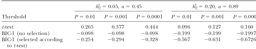
TABLE A1
Selection bias in estimation of effects of allelic substitution, for single markert-test analysis and model averaging using BIC-␦
h2
Q⫽0.05,a⫽0.45 h2Q⫽0.20,a⫽0.89
Threshold P⫽0.01 P⫽0.001 P⫽0.0001 P⫽0.01 P⫽0.001 P⫽0.0001
t-test 0.265 0.377 0.444 0.096 0.127 0.160
BIC-1 (no selection) ⫺0.098 ⫺0.098 ⫺0.098 ⫺0.199 ⫺0.199 ⫺0.1997
BIC-1 (selected according ⫺0.254 ⫺0.294 ⫺0.328 ⫺0.567 ⫺0.631 ⫺0.6726
tot-test)
Bias in estimation of effects of allelic substitution in units of one phenotypic standard deviation from 2000 simulations, each with 100 progeny with six markers on a single chromosome of length 120 cM, is shown. A QTL was present with probability 0.53, and if present had QTL heritabilityh2
Q⫽0.05 orh2Q⫽0.2, is given for thet-test, model averaging using BIC, and model averaging conditional on selection by thet-test. Selection was for various thresholds corresponding toP⫽0.01, 0.001, and 0.0001.
di ⫽di,j⫽dj⫻(1⫺ 2rij). nificant markers only. This may be an artifact of the fact that as the threshold increases, the simulated QTL, Thus selection bias indˆiisⵑ1/(1⫺2rij). Furthermore, if selected, is more likely to be at or near the marker assuming modelMk(i)we estimate under consideration, so the effect is larger; hence the
potential shrinkage toward zero is larger.
dˆj ⫽dˆi ⫻(1⫺ 2rij).
Selection bias and model averaging—summary: Thus assuming Mk(i) when Mk(j) is the true model 1. Selection bias occurs when the same data are used
induces a relative bias of the order of (1⫺2rij)2in the
to select a regression model and to estimate the
coef-ratio of dˆi/dˆj. ficients (here marker effects) in the model.
If the model selected is the null modelM0 with no 2. Selection bias occurs because expected values of
esti-QTL, the estimated effect is zero.
mates of the effect of allelic substitution at a marker Selection bias and model averaging—a simulation
are always greater under the model with that marker study:For each ofh2Q⫽0.05 andh2
Q⫽0.2, 2000 simulated selected than under any other single-marker model data sets were generated each with 100 backcross prog- or the null model.
eny, with 0 (probability 0.53) or 1 QTL explaining pro- 3. Estimates of allelic substitution at a marker are unbi-portionh2
Qof total variance, randomly placed on a chro- ased, if the true model is known, or selected with mosome of length 120 cM with six markers evenly independent data.
spaced at positions 10, 30, 50, 70, 90, and 110 cM. The 4. Selection bias is not a problem if Bayesian model size of the QTL effect if present always had a positive averaging is used. The model-averaged Bayesian esti-sign, corresponding to a QTL effect ofa⫽0.45 (ora⫽ mates are not unbiased under any assumed QTL
0.89 in units of 1 phenotypic standard deviation). The configuration but are the average of unbiased esti-analysis used model averaging with BIC-␦, with ␦ ⫽ 1 mates under various models, averaged according to and prior probability ⫽0.1 for a marker to be selected. the posterior probability that each model is the true Table A1 gives bias in units of 1 phenotypic standard model. From observation (2) it follows that model-deviation for the single-markert-test and model averag- averaging estimates of QTL effects are shrunk toward
ing using BIC. zero. The amount of shrinkage reduces with the
pre-The fourth row of Table A1 is the average “bias” using cision with which the QTL location can be deter-model averaging with BIC-1 (␦ ⫽ 1). A negative bias mined.
(shrinkage toward zero) is expected with the Bayesian 5. The Bayesian method can be applied even if a previ-method if there is any model uncertainty. ous hypothesis test or tests have selected a chromo-The fifth row of Table A1 is the average bias using some or region (as was the case for linkage group 3 in model averaging conditional on markers being selected this study). This is because the posterior probability by thet-test method (not something we would necessar- distribution for that chromosome or region depends ily advocate). Interestingly, while the bias for thet-test only on the data through the likelihood function method as used increases with selection intensity, as and the prior probability for that chromosome or expected, the bias for BIC actually decreases (increases region.