Optimal Placement of IPFC Using Genetic Algorithm for Transmission Line Loss Reduction

Optimal Placement of IPFC Using Genetic

Algorithm for Transmission Line Loss

Reduction

V. Suryanarayanareddy1, Dr.A.lakshmidevi2

M.Tech Student, Dept. of EEE, SVU College, Andhra Pradesh, India1

Professor (M.Tech, PhD), Dept. of EEE, SVU College, Andhra Pradesh, India2

ABSTRACT:The electrical energy which is obtained from generating plant is transfer from one place to another through the transmission lines. This energy is effectively controlled by the flexible AC transmission systems. But the interline power flow controller gives the best results for compare to the other controllers. The establishment of new transmission line is not easy. The many factor effects at the time of newtransmission line construction. In this paper explain the MATLAB code of interline power flow controller. Because it is a series connected device. This device controls the active and reactive power in multiline system. This paper describes about the,how to reduce the line loss in transmission system .Its explain by using genetic algorithm method .It is connected series in transmission line so its became a main advantage of this device.

KEYWORDS:IPFC , genetic algorithm , multiline system , line loss

I.INTRODUCTION

For controlling active and reactive power in line there are so many FACTs devices is there. They are static synchronous compensator (STATCOM), static var compensator (SVC), but the second generation devices are mostly used. These FACTs devices are unified power flow controller (UPFC), static synchronous series compensator (SSSC) and interline power flow controller (IPFC). From all these, the interline power flow controller are the best device as compare to the other controllers. In the interline power flow controller consist a two voltage source converter and sharing a common Capacitor for absorbing the transient unbalance reactive power. The voltage source converters connected to line throw the coupling transformer.

Where the reactive power is individual voltage Source. Injecting converter to regulate the active power in the line. The first voltage source converter regulates the DC voltage and second converter is to maintain the reactive power in the lines. Basically the working of interline power flow controller are to control the both active and reactive power in line. IPFC having the capacity to transfer the power from under load into overload . In this paper, the MATLAB model of interline power flow controller is formed by implementing Genetic algorithm and result are also described in the MATLAB.

II. BASIC PRINCIPAL OF INTERLINE POWER FLOW CONTROLLER

power which transferred between the two Voltage sources converters is through the DC link. This DC Link is bidirectional link.

Figure .1 schematic representation of IPFC

The power flow model of a interline power flow controller is given is shown in below figure.2.It is also applied in power quality improvement of a system in multiline.

Figure 2.power flow model of the ipfc II.IPOWER INJECTION MODEL OF IPFC

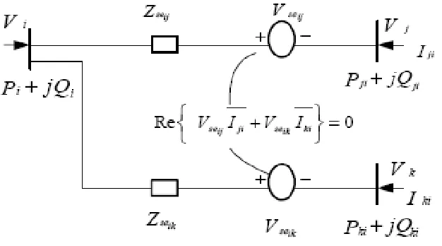
The power injection model of IPFC is useful for calculating the injecting active power, voltage and voltage angle in each bus. The power calculation is based on the NR load flow algorithm. It is used to check the loss variation before and after connecting IPFC. The equivalent circuit for the power injection model of IPFC is shown in Figure.2.

In this mathematical model Va, Vb and VC are the bus voltages of bus a, b and c respectively. Under normal conditions,

real power across the two transmission lines is Re {VABIab Vac I ac} 0. The impedance

value of this two line is Zab and Zac. The current between the buses VA and Vb is Iab and Iac . The power flow equation of

= −



( cos( − ) +ℎ sin( − ))−



( cos( − ) +ℎ sin( − )) (1)

= ℎ −



( cos( − ) +ℎ sin( − ))−



cos( − +ℎ sin( − ))(2)

Where

V: is the voltage magnitude Is the bus angle

Is the magnitude injected voltage : Angle of injected voltage

III .GENETIC ALGORITHM

In this chapter discussing about Genetic algorithm (GA).It is a one of the method which is depends on mechanical artificial genetics. GA actually used to compare the similarity of two things.(direct analogy).It is also used to optimize the applied solution by using the biological method it is explained by Darwin.Basically it is used in different applications its gives a exact result compare to other methods for solving specific error using GA.In this fitness function are used because to obtain the different possible solutions .In below showing the algorithm its compare each possible solution and gives the best one .This is about the genetic algorithm

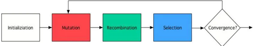
III.I Basic flowchart for GA

Figure 3. Flow chart for GA III.II Algorithm for GA

In this they are three steps shown in below

A. Initialization

B. Mutation

C. Crossover

D. Selection

J(x) =



 n

j1

( ) (1)

a. Initialization

first step is to initialize the solution vectors Xj, G = {x1j, G,….,xDj,G} j=1 ,n (2)

Wheren ,G ,D,are populations ,generators ,control parameters.The below equation shows the random solution Xij, 0 = Ximin + rand (0, 1). (Ximax - Ximin) i = 1, D (3)

Here ≤ , ≤

b. Mutation

Here we are applying mutation operation to produce mutant vector ( , = [ , , , , … . . , , ]) belongs with

target vector. The mutation equation is shown in below

M j, G= Xr1j, G + F(X ri2, G – X ri3, G) i = 1…n (4) Xrj, G is target vectors ,F is a positive scaling factor

c. Crossover

This operation is used for producing trail vector , = , , , , … , cross over operation of a binomial equation is

shown in below

MIj, G if (rand I [0, 1) ≤ CR or (i=irand))

Uij, G I = xij, G other wise

d. Selection

by using the mutation and target vector control parameters are interchanging .After changing of target vector (Xj, G1)

is

Xj, G+1 = U j, Gif f (Uj, G) ≤ f (xj, G) (5)

X j, G otherwise

These iterations are repeated until the loss is

IV. POWER FLOW CALCULATION OF IPFC

The power flow calculations of IPFC are performed using basic load flow formulas. Using the basic formulas real power, bus voltage and voltage angles are calculated for IPFC connected lines. Thus the improvement in real power and loss variation of the IPFC connected transmission lines are determined easily. Once the real power and transmission losses are determined the amount of IPFC stabilized losses can be calculated. Several methods are available to solve the power flow of a system and NR is the one of the most popular methods. The general power flow solution of Newton Raphson (NR) is explained as follows.

1. Initialize all the unknown variables such as voltage magnitude is set as 1 p.u and voltage angle is set as zero. 2. Calculate the Y-bus matrix.

3. to solving the power balance equation using voltage magnitude and angle. 4. Create Jacobian matrix corresponding to the power mismatch.

5. set the determined voltage magnitude and voltage angle.

6. in this step we have to solve change in voltage angle and magnitude. 7. Update the voltage magnitude and angle.

8. By checking ending conditions, if it obtain desire solution then end o, else go to step 3.

This process is continued until a predetermined condition is satisfied. A common ending condition is to removing if the power mismatch equation is below the tolerance value.

V. RESULTS AND DISCUSSION

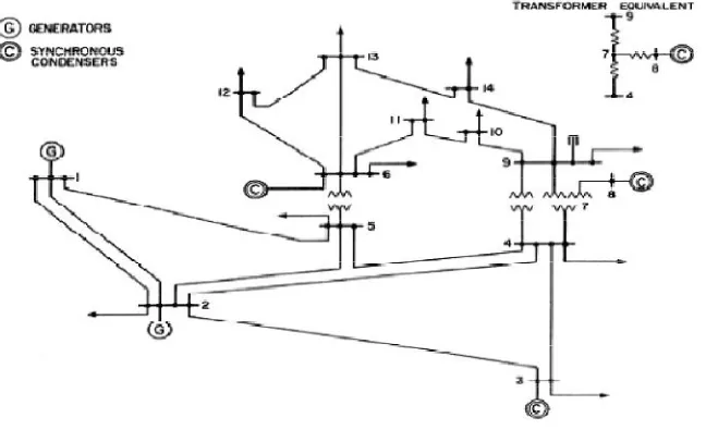
are load data of the standard bus system before connecting IPFC. Table 2 are loaddata of IPFC connected in two lines .The two lines selected are from 3 ,4and5 buses.Table 3 are load data of IPFC connected in multi lines. The IPFC connected lines are selected from bus number 6 to 11

Figure : IEEE 14 bus system

In this bus data taken as standard IEEE data .before applying ipfctotal real and reactive power is 5199.3 and 23887.7 and when ipfc applying at 3-5 busses the real and reactive power is 4065.3 and 21345.7 and at 6-11 busses real and reactive is 3382.2 and 18806.4 .after placing ipfc at 3-5 busses the loss percentage of real and reactive power is 18% and 5% . After placing at 6-11 real and reactive power loss is 39% and19%. Efficiency is increased by placing the ipfc at different busses.

Table : Total loss with loss percentage

WITHOUT IPFC WITH IPFC BETWEEN 3-5

WITH IPFC BETWEEN 6-11

PERCENTAGE OF LOSS REDUCTION

P(KW )

Q(KVAr )

P Q P Q p Q

5199.3 23887.7 4065.3 21345.7 3382.2 18806.4 39% 19%

VI .CONCLUSIONS

In this paper shows about the IPFC how it reduces the line loss in transmission system .it is a multiline device used to control the reactive and real power in multiline machine. In this genetic algorithm method is used to control the ipfc parameters for minimizing the loss . This paper is tested in multiline system .these results indicated ipfc is reduce total active and reactive power

REFERENCES

2. N.G. Hingorani and L. Gyugyi, “Understanding FACTS: concepts and technology of flexible ac transmission systems”, IEEE Press, NY, 1999 3. L. Gyugyi, K.K.Sen, C.D.Schauder, “The interline power flow controller concept: A new approach to power flow management in transmission

line system”, IEEE Trans. on Power Delivery, Vol. 14, No. 3, 1999, pp. 1115-1123.

4. Z.Haibo, Z .Lizi And M. Fanling , " Reactive poweroptimization based on genetic algorithm ", International power conference on power system