Text Classification Improved by Integrating Bidirectional LSTM with Two dimensional Max Pooling

Text Classification Improved by Integrating Bidirectional LSTM

with Two-dimensional Max Pooling

Peng Zhou1_{, Zhenyu Qi}1∗_{, Suncong Zheng}1_{, Jiaming Xu}1_{, Hongyun Bao}1_{, Bo Xu}1,2

(1) Institute of Automation, Chinese Academy of Sciences (2) Center for Excellence in Brain Science and Intelligence Technology

{zhoupeng2013, zhenyu.qi, zhengsuncong,

jiaming.xu, hongyun.bao, xubo}@ia.ac.cn

Abstract

Recurrent Neural Network (RNN) is one of the most popular architectures used in Natural Lan-guage Processsing (NLP) tasks because its recurrent structure is very suitable to process variable-length text. RNN can utilize distributed representations of words by first converting the tokens comprising each text into vectors, which form a matrix. And this matrix includes two dimen-sions: the time-step dimension and the feature vector dimension. Then most existing models usually utilize one-dimensional (1D) max pooling operation or attention-based operation only on the time-step dimension to obtain a fixed-length vector. However, the features on the feature vector dimension are not mutually independent, and simply applying 1D pooling operation over the time-step dimension independently may destroy the structure of the feature representation. On the other hand, applying two-dimensional (2D) pooling operation over the two dimensions may sample more meaningful features for sequence modeling tasks. To integrate the features on both dimensions of the matrix, this paper explores applying 2D max pooling operation to obtain a fixed-length representation of the text. This paper also utilizes 2D convolution to sample more meaningful information of the matrix. Experiments are conducted on six text classification tasks, including sentiment analysis, question classification, subjectivity classification and newsgroup classification. Compared with the state-of-the-art models, the proposed models achieve excellent performance on 4 out of 6 tasks. Specifically, one of the proposed models achieves highest accu-racy on Stanford Sentiment Treebank binary classification and fine-grained classification tasks.

1 Introduction

Text classification is an essential component in many NLP applications, such as sentiment analysis (Socher et al., 2013), relation extraction (Zeng et al., 2014) and spam detection (Wang, 2010). There-fore, it has attracted considerable attention from many researchers, and various types of models have been proposed. As a traditional method, the bag-of-words (BoW) model treats texts as unordered sets of words (Wang and Manning, 2012). In this way, however, it fails to encode word order and syntactic feature.

Recently, order-sensitive models based on neural networks have achieved tremendous success for text classification, and shown more significant progress compared with BoW models. The challenge for textual modeling is how to capture features for different text units, such as phrases, sentences and documents. Benefiting from its recurrent structure, RNN, as an alternative type of neural networks, is very suitable to process the variable-length text.

RNN can capitalize on distributed representations of words by first converting the tokens compris-ing each text into vectors, which form a matrix. This matrix includes two dimensions: the time-step dimension and the feature vector dimension, and it will be updated in the process of learning feature representation. Then RNN utilizes 1D max pooling operation (Lai et al., 2015) or attention-based oper-ation (Zhou et al., 2016), which extracts maximum values or generates a weighted representoper-ation over

∗

Correspondence author: [email protected]

This work is licenced under a Creative Commons Attribution 4.0 International Licence. Licence details: http:// creativecommons.org/licenses/by/4.0/

the time-step dimension of the matrix, to obtain a fixed-length vector. Both of the two operators ignore features on the feature vector dimension, which maybe important for sentence representation, therefore the use of 1D max pooling and attention-based operators may pose a serious limitation.

Convolutional Neural Networks (CNN) (Kalchbrenner et al., 2014; Kim, 2014) utilizes 1D convolution to perform the feature mapping, and then applies 1D max pooling operation over the time-step dimension to obtain a fixed-length output. However the elements in the matrix learned by RNN are not independent, as RNN reads a sentence word by word, one can effectively treat the matrix as an ’image’. Unlike in NLP, CNN in image processing tasks (LeCun et al., 1998; Krizhevsky et al., 2012) applies 2D convolution and 2D pooling operation to get a representation of the input. It is a good choice to utilize 2D convolution and 2D pooling to sample more meaningful features on both the time-step dimension and the feature vector dimension for text classification.

Above all, this paper proposes Bidirectional Long Short-Term Memory Networks with Two-Dimensional Max Pooling (BLSTM-2DPooling) to capture features on both the time-step dimension and the feature vector dimension. It first utilizes Bidirectional Long Short-Term Memory Networks (BLSTM) to transform the text into vectors. And then 2D max pooling operation is utilized to obtain a fixed-length vector. This paper also applies 2D convolution (BLSTM-2DCNN) to capture more mean-ingful features to represent the input text.

The contributions of this paper can be summarized as follows:

• This paper proposes a combined framework, which utilizes BLSTM to capture long-term sentence

dependencies, and extracts features by 2D convolution and 2D max pooling operation for sequence modeling tasks. To the best of our knowledge, this work is the first example of using 2D convolution and 2D max pooling operation in NLP tasks.

• This work introduces two combined models BLSTM-2DPooling and BLSTM-2DCNN, and

veri-fies them on six text classification tasks, including sentiment analysis, question classification, sub-jectivity classification, and newsgroups classification. Compared with the state-of-the-art models,

BLSTM-2DCNN achieves excellent performance on4out of6tasks. Specifically, it achieves

high-est accuracy on Stanford Sentiment Treebank binary classification and fine-grained classification tasks.

• To better understand the effect of 2D convolution and 2D max pooling operation, this paper conducts

experiments on Stanford Sentiment Treebank fine-grained task. It first depicts the performance of the proposed models on different length of sentences, and then conducts a sensitivity analysis of 2D filter and max pooling size.

The remainder of the paper is organized as follows. In Section 2, the related work about text classifi-cation is reviewed. Section 3 presents the BLSTM-2DCNN architectures for text classificlassifi-cation in detail. Section 4 describes details about the setup of the experiments. Section 5 presents the experimental re-sults. The conclusion is drawn in the section 6.

2 Related Work

Deep learning based neural network models have achieved great improvement on text classification tasks. These models generally consist of a projection layer that maps words of text to vectors. And then combine the vectors with different neural networks to make a fixed-length representation. According

to the structure, they may divide into four categories: Recursive Neural Networks (RecNN1_{), RNN,}

CNN and other neural networks.

Recursive Neural Networks: RecNN is defined over recursive tree structures. In the type of recursive models, information from the leaf nodes of a tree and its internal nodes are combined in a bottom-up manner. Socher et al. (2013) introduced recursive neural tensor network to build representations of phrases and sentences by combining neighbour constituents based on the parsing tree. Irsoy and Cardie

(2014) proposed deep recursive neural network, which is constructed by stacking multiple recursive layers on top of each other, to modeling sentence.

Recurrent Neural Networks: RNN has obtained much attention because of their superior ability to preserve sequence information over time. Tang et al. (2015) developed target dependent Long Short-Term Memory Networks (LSTM (Hochreiter and Schmidhuber, 1997)), where target information is auto-matically taken into account. Tai et al. (2015) generalized LSTM to Tree-LSTM where each LSTM unit gains information from its children units. Zhou et al. (2016) introduced BLSTM with attention mech-anism to automatically select features that have a decisive effect on classification. Yang et al. (2016) introduced a hierarchical network with two levels of attention mechanisms, which are word attention and sentence attention, for document classification. This paper also implements an attention-based model BLSTM-Att like the model in Zhou et al. (2016).

Convolution Neural Networks: CNN (LeCun et al., 1998) is a feedforward neural network with 2D convolution layers and 2D pooling layers, originally developed for image processing. Then CNN is ap-plied to NLP tasks, such as sentence classification (Kalchbrenner et al., 2014; Kim, 2014), and relation classification (Zeng et al., 2014). The difference is that the common CNN in NLP tasks is made up of 1D convolution layers and 1D pooling layers. Kim (2014) defined a CNN architecture with two

chan-nels. Kalchbrenner et al. (2014) proposed a dynamick-max pooling mechanism for sentence modeling.

(Zhang and Wallace, 2015) conducted a sensitivity analysis of one-layer CNN to explore the effect of architecture components on model performance. Yin and Sch¨utze (2016) introduced multichannel em-beddings and unsupervised pretraining to improve classification accuracy. (Zhang and Wallace, 2015) conducted a sensitivity analysis of one-layer CNN to explore the effect of architecture components on model performance.

Usually there is a misunderstanding that 1D convolutional filter in NLP tasks has one dimension.

Actually it has two dimensions (k, d), wherek,d∈R. Asdis equal to the word embeddings sizedw_,

the window slides only on the time-step dimension, so the convolution is usually called 1D convolution.

Whiledin this paper varies from 2 todw_{, to avoid confusion with common CNN, the convolution in this}

work is named as 2D convolution. The details will be described in Section 3.2.

Other Neural Networks: In addition to the models described above, lots of other neural networks have been proposed for text classification. Iyyer et al. (2015) introduced a deep averaging network, which fed an unweighted average of word embeddings through multiple hidden layers before classifica-tion. Zhou et al. (2015) used CNN to extract a sequence of higher-level phrase representations, then the representations were fed into a LSTM to obtain the sentence representation.

The proposed model BLSTM-2DCNN is most relevant to DSCNN (Zhang et al., 2016) and RCNN (Wen et al., 2016). The difference is that the former two utilize LSTM, bidirectional RNN respectively, while this work applies BLSTM, to capture long-term sentence dependencies. After that the former two both apply 1D convolution and 1D max pooling operation, while this paper uses 2D convolution and 2D max pooling operation, to obtain the whole sentence representation.

3 Model

As shown in Figure 1, the overall model consists of four parts: BLSTM Layer, Two-dimensional Con-volution Layer, Two dimensional max pooling Layer, and Output Layer. The details of different compo-nents are described in the following sections.

3.1 BLSTM Layer

LSTM was firstly proposed by Hochreiter and Schmidhuber (1997) to overcome the gradient vanishing problem of RNN. The main idea is to introduce an adaptive gating mechanism, which decides the degree to keep the previous state and memorize the extracted features of the current data input. Given a sequence

S ={x1, x2, . . . , xl}, wherelis the length of input text, LSTM processes it word by word. At time-step

left context word embedding ...

right context

BLSTM Layer Two-dimensional

Convolution Layer

Two-dimensional Max Pooling Layer

Output Layer

Figure 1: A BLSTM-2DCNN for the seven word input sentence. Word embeddings have size 3, and BLSTM has 5 hidden units. The height and width of convolution filters and max pooling operations are 2, 2 respectively.

   

it

ft

ot

ˆ

ct    =

   

σ σ σ

tanh

  

W ·[ht−1, xt] (1)

ct = ft⊙ct−1+it⊙cˆt (2)

ht = ot⊙tanh(ct) (3)

wherextis the input at the current time-step,i,f andois the input gate activation, forget gate activation

and output gate activation respectively,cˆis the current cell state,σdenotes the logistic sigmoid function

and⊙denotes element-wise multiplication.

For the sequence modeling tasks, it is beneficial to have access to the past context as well as the future context. Schuster and Paliwal (1997) proposed BLSTM to extend the unidirectional LSTM by introducing a second hidden layer, where the hidden to hidden connections flow in opposite temporal order. Therefore, the model is able to exploit information from both the past and the future.

In this paper, BLSTM is utilized to capture the past and the future information. As shown in Figure 1, the network contains two sub-networks for the forward and backward sequence context respectively.

The output of theith_{word is shown in the following equation:}

hi= [−→hi ⊕←h−i] (4)

Here, element-wise sum is used to combine the forward and backward pass outputs.

3.2 Convolutional Neural Networks

Since BLSTM has access to the future context as well as the past context, hi is related to all the other

3.2.1 Two-dimensional Convolution Layer

A matrix H = {h1, h2, . . . , hl}, H ∈ Rl×dw, is obtained from BLSTM Layer, wheredw is the size

of word embeddings. Then narrow convolution is utilized (Kalchbrenner et al., 2014) to extract local

features overH. A convolution operation involves a 2D filterm∈Rk×d_{, which is applied to a window}

of k words and d feature vectors. For example, a feature oi,j is generated from a window of vectors

Hi:i+k−1, j:j+d−1by

oi,j =f(m·Hi:i+k−1, j:j+d−1+b) (5)

whereiranges from 1 to(l−k+ 1),jranges from 1 to(dw _{−d+ 1),·represents dot product,b ∈R}

is a bias and anf is a non-linear function such as the hyperbolic tangent. This filter is applied to each

possible window of the matrixHto produce a feature mapO:

O= [o1,1, o1,2,· · · , ol−k+1,dw_−d+1] (6)

withO ∈ R(l−k+1)×(dw_−d+1)

. It has described the process of one convolution filter. The convolution layer may have multiple filters for the same size filter to learn complementary features, or multiple kinds of filter with different size.

3.2.2 Two-dimensional Max Pooling Layer

Then 2D max pooling operation is utilized to obtain a fixed length vector. For a 2D max pooling p ∈

Rp1×p2, it is applied to each possible window of matrix O to extract the maximum value:

pi,j=down(Oi:i+p1, j:j+p2) (7)

wheredown(·)represents the 2D max pooling function,i= (1,1 +p1,· · · ,1 + (l−k+ 1/p1−1)·p1), andj= (1, 1+p2,· · · ,1+(dw−d+1/p2−1)·p2). Then the pooling results are combined as follows:

h∗ _{= [p}

1,1, p1,1+p2,· · · , p1+(l−k+1/p1−1)·p1,1+(dw−d+1/p2−1)·p2] (8)

whereh∗_{∈R, and the length ofh}∗_{is⌊l−k+ 1/p1⌋ × ⌊d}w_{−d+ 1/p2⌋.}

3.3 Output Layer

For text classification, the output h∗ _{of 2D Max Pooling Layer is the whole representation of the input}

textS. And then it is passed to a softmax classifier layer to predict the semantic relation labelyˆfrom a discrete set of classesY. The classifier takes the hidden stateh∗_{as input:}

ˆ

p(y|s) = softmaxW(s)_h∗_+b(s) ₍₉₎

ˆ

y = arg max

y pˆ(y|s) (10)

A reasonable training objective to be minimized is the categorical cross-entropy loss. The loss is calculated as a regularized sum:

J(θ) =−_m1 Xm i=1

tilog(yi) +λkθk2F (11)

wheret∈Rm_{is the one-hot represented ground truth,y∈R}m_{is the estimated probability for each class}

by softmax,mis the number of target classes, andλis an L2 regularization hyper-parameter. Training

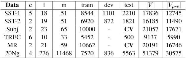
Data c l m train dev test |V| |Vpre|

SST-1 5 18 51 8544 1101 2210 17836 12745

SST-2 2 19 51 6920 872 1821 16185 11490

Subj 2 23 65 10000 - CV 21057 17671

TREC 6 10 33 5452 - 500 9137 5990

MR 2 21 59 10662 - CV 20191 16746

20Ng 4 276 11468 7520 836 5563 51379 30575

Table 1: Summary statistics for the datasets. c: number of target classes, l: average sentence length, m: maximum sentence length, train/dev/test: train/development/test set size, |V|: vocabulary size, |Vpre|:

number of words present in the set of pre-trained word embeddings,CV: 10-fold cross validation.

4 Experimental Setup 4.1 Datasets

The proposed models are tested on six datasets. Summary statistics of the datasets are in Table 1.

• MR2_{: Sentence polarity dataset from Pang and Lee (2005). The task is to detect positive/negative}

reviews.

• SST-13_{: Stanford Sentiment Treebank is an extension of MR from Socher et al. (2013). The aim is}

to classify a review as fine-grained labels (very negative, negative, neutral, positive, very positive).

• SST-2: Same as SST-1 but with neutral reviews removed and binary labels (negative, positive). For both experiments, phrases and sentences are used to train the model, but only sentences are scored at test time (Socher et al., 2013; Le and Mikolov, 2014). Thus the training set is an order of magnitude larger than listed in table 1.

• Subj4_{: Subjectivity dataset (Pang and Lee, 2004). The task is to classify a sentence as being}

subjective or objective.

• TREC5_{: Question classification dataset (Li and Roth, 2002). The task involves classifying a}

ques-tion into 6 quesques-tion types (abbreviaques-tion, descripques-tion, entity, human, locaques-tion, numeric value).

• 20Newsgroups6_{: The 20Ng dataset contains messages from twenty newsgroups. We use the bydate}

version preprocessed by Cachopo (2007). We select four major categories (comp, politics, rec and religion) followed by Hingmire et al. (2013).

4.2 Word Embeddings

The word embeddings are pre-trained on much larger unannotated corpora to achieve better generaliza-tion given limited amount of training data (Turian et al., 2010). In particular, our experiments utilize

the GloVe embeddings7 _{trained by Pennington et al. (2014) on 6 billion tokens of Wikipedia 2014 and}

Gigaword 5. Words not present in the set of pre-trained words are initialized by randomly sampling from uniform distribution in[−0.1,0.1]. The word embeddings are fine-tuned during training to improve the performance of classification.

2_{https://www.cs.cornell.edu/people/pabo/movie-review-data/} 3_{http://nlp.stanford.edu/sentiment/}

4_{http://www.cs.cornell.edu/people/pabo/movie-review-data/} 5_{http://cogcomp.cs.illinois.edu/Data/QA/QC/}

4.3 Hyper-parameter Settings

For datasets without a standard development set we randomly select 10% of the training data as the

development set. The evaluation metric of the 20Ng is the Macro-F1 measure followed by the state-of-the-art work and the other five datasets use accuracy as the metric. The final hyper-parameters are as follows.

The dimension of word embeddings is 300, the hidden units of LSTM is 300. We use 100 convo-lutional filters each for window sizes of (3,3), 2D pooling size of (2,2). We set the mini-batch size as 10 and the learning rate of AdaDelta as the default value 1.0. For regularization, we employ Dropout operation (Hinton et al., 2012) with dropout rate of 0.5 for the word embeddings, 0.2 for the BLSTM

layer and 0.4 for the penultimate layer, we also use l2 penalty with coefficient10−5_{over the parameters.}

These values are chosen via a grid search on the SST-1 development set. We only tune these hyper-parameters, and more finer tuning, such as using different numbers of hidden units of LSTM layer, or using wide convolution (Kalchbrenner et al., 2014), may further improve the performance.

5 Results

5.1 Overall Performance

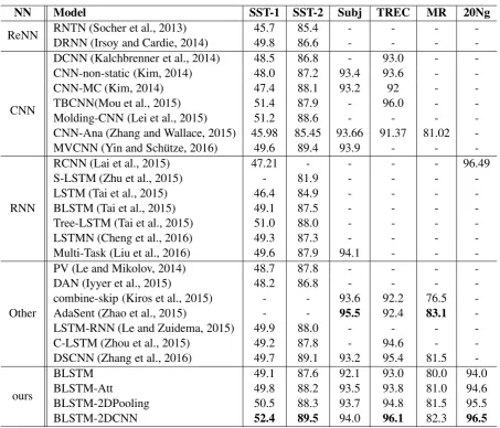
This work implements four models, BLSTM, BLSTM-Att, BLSTM-2DPooling, and BLSTM-2DCNN. Table 2 presents the performance of the four models and other state-of-the-art models on six classification tasks. The BLSTM-2DCNN model achieves excellent performance on 4 out of 6 tasks. Especially, it

achieves52.4%and89.5%test accuracies on SST-1 and SST-2 respectively.

BLSTM-2DPooling performs worse than the state-of-the-art models. While we expect performance gains through the use of 2D convolution, we are surprised at the magnitude of the gains. BLSTM-CNN beats all baselines on SST-1, SST-2, and TREC datasets. As for Subj and MR datasets, BLSTM-2DCNN gets a second higher accuracies. Some of the previous techniques only work on sentences, but not paragraphs/documents with several sentences. Our question becomes whether it is possible to use our models for datasets that have a substantial number of words, such as 20Ng and where the content consists of many different topics. For that purpose, this paper tests the four models on document-level dataset 20Ng, by treating the document as a long sentence. Compared with RCNN (Lai et al., 2015), BLSTM-2DCNN achieves a comparable result.

Besides, this paper also compares with ReNN, RNN, CNN and other neural networks:

• Compared with ReNN, the proposed two models do not depend on external language-specific

fea-tures such as dependency parse trees.

• CNN extracts features from word embeddings of the input text, while BLSTM-2DPooling and

BLSTM-2DCNN captures features from the output of BLSTM layer, which has already extracted features from the original input text.

• BLSTM-2DCNN is an extension of BLSTM-2DPooling, and the results show that BLSTM-2DCNN

can capture more dependencies in text.

• AdaSent utilizes a more complicated model to form a hierarchy of representations, and it

outper-forms BLSTM-2DCNN on Subj and MR datasets. Compared with DSCNN (Zhang et al., 2016), BLSTM-2DCNN outperforms it on five datasets.

Compared with these results, 2D convolution and 2D max pooling operation are more effective for modeling sentence, even document. To better understand the effect of 2D operations, this work conducts a sensitivity analysis on SST-1 dataset.

5.2 Effect of Sentence Length

NN Model SST-1 SST-2 Subj TREC MR 20Ng

ReNN RNTN (Socher et al., 2013)_{DRNN (Irsoy and Cardie, 2014)} 45.7_49.8 85.4_86.6 -_- -_- -_- -

-CNN

DCNN (Kalchbrenner et al., 2014) 48.5 86.8 - 93.0 -

-CNN-non-static (Kim, 2014) 48.0 87.2 93.4 93.6 -

-CNN-MC (Kim, 2014) 47.4 88.1 93.2 92 -

-TBCNN(Mou et al., 2015) 51.4 87.9 - 96.0 -

-Molding-CNN (Lei et al., 2015) 51.2 88.6 - - -

-CNN-Ana (Zhang and Wallace, 2015) 45.98 85.45 93.66 91.37 81.02

-MVCNN (Yin and Sch¨utze, 2016) 49.6 89.4 93.9 - -

-RNN

RCNN (Lai et al., 2015) 47.21 - - - - 96.49

S-LSTM (Zhu et al., 2015) - 81.9 - - -

-LSTM (Tai et al., 2015) 46.4 84.9 - - -

-BLSTM (Tai et al., 2015) 49.1 87.5 - - -

-Tree-LSTM (Tai et al., 2015) 51.0 88.0 - - -

-LSTMN (Cheng et al., 2016) 49.3 87.3 - - -

-Multi-Task (Liu et al., 2016) 49.6 87.9 94.1 - -

-Other

PV (Le and Mikolov, 2014) 48.7 87.8 - - -

-DAN (Iyyer et al., 2015) 48.2 86.8 - - -

-combine-skip (Kiros et al., 2015) - - 93.6 92.2 76.5

-AdaSent (Zhao et al., 2015) - - 95.5 92.4 83.1

-LSTM-RNN (Le and Zuidema, 2015) 49.9 88.0 - - -

-C-LSTM (Zhou et al., 2015) 49.2 87.8 - 94.6 -

-DSCNN (Zhang et al., 2016) 49.7 89.1 93.2 95.4 81.5

-ours

BLSTM 49.1 87.6 92.1 93.0 80.0 94.0

BLSTM-Att 49.8 88.2 93.5 93.8 81.0 94.6

BLSTM-2DPooling 50.5 88.3 93.7 94.8 81.5 95.5

BLSTM-2DCNN 52.4 89.5 94.0 96.1 82.3 96.5

Table 2: Classification results on several standard benchmarks. RNTN: Recursive deep models for

se-mantic compositionality over a sentiment treebank (Socher et al., 2013). DRNN: Deep recursive neural

networks for compositionality in language (Irsoy and Cardie, 2014). DCNN: A convolutional neural

network for modeling sentences (Kalchbrenner et al., 2014). CNN-nonstatic/MC: Convolutional

neu-ral networks for sentence classification (Kim, 2014). TBCNN: Discriminative neural sentence

model-ing by tree-based convolution (Mou et al., 2015). Molding-CNN: Molding CNNs for text: non-linear,

non-consecutive convolutions (Lei et al., 2015). CNN-Ana: A Sensitivity Analysis of (and

Practition-ers’ Guide to) Convolutional Neural Networks for Sentence Classification (Zhang and Wallace, 2015).

MVCNN: Multichannel variable-size convolution for sentence classification (Yin and Sch¨utze, 2016).

RCNN: Recurrent Convolutional Neural Networks for Text Classification (Lai et al., 2015). S-LSTM:

Long short-term memory over recursive structures (Zhu et al., 2015). LSTM/BLSTM/Tree-LSTM:

Improved semantic representations from tree-structured long short-term memory networks (Tai et al.,

2015). LSTMN: Long short-term memory-networks for machine reading (Cheng et al., 2016).

Multi-Task: Recurrent Neural Network for Text Classification with Multi-Task Learning (Liu et al., 2016).

PV: Distributed representations of sentences and documents (Le and Mikolov, 2014). DAN: Deep

un-ordered composition rivals syntactic methods for text classification (Iyyer et al., 2015). combine-skip:

skip-thought vectors (Kiros et al., 2015). AdaSent: Self-adaptive hierarchical sentence model (Zhao

et al., 2015). LSTM-RNN: Compositional distributional semantics with long short term memory (Le

and Zuidema, 2015). C-LSTM: A C-LSTM Neural Network for Text Classification (Zhou et al., 2015).

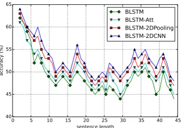
0 5 10 15 20 25 30 35 40 45 sentence length 40 45 50 55 60 65 ac cu ra cy ( % ) BLSTM BLSTM-Att BLSTM-2DPooling BLSTM-2DCNN

Figure 2: Fine-grained sentiment classification

accuracyvs.sentence length.

c_2 c_3 c_4 c_5 c_6 2D filter size

49.0 49.5 50.0 50.5 51.0 51.5 52.0 52.5 53.0 ac cu ra cy ( % )

Figure 3: Prediction accuracy with different size of 2D filter and 2D max pooling.

longer than 45 words. The accuracy here is the average value of the sentences with length in the window

[l−2, l+ 2]. Each data point is a mean score over 5 runs, and error bars have been omitted for clarity. It is found that both BLSTM-2DPooling and BLSTM-2DCNN outperform the other two models. This suggests that both 2D convolution and 2D max pooling operation are able to encode semantically-useful structural information. At the same time, it shows that the accuracies decline with the length of sen-tences increasing. In future work, we would like to investigate neural mechanisms to preserve long-term dependencies of text.

5.3 Effect of 2D Convolutional Filter and 2D Max Pooling Size

We are interested in what is the best 2D filter and max pooling size to get better performance. We conduct experiments on SST-1 dataset with BLSTM-2DCNN and set the number of feature maps to 100.

To make it simple, we set these two dimensions to the same values, thus both the filter and the pooling are square matrices. For the horizontal axis, c means 2D convolutional filter size, and the five different color bar charts on each c represent different 2D max pooling size from 2 to 6. Figure 3 shows that dif-ferent size of filter and pooling can get difdif-ferent accuracies. The best accuracy is 52.6 with 2D filter size (5,5) and 2D max pooling size (5,5), this shows that finer tuning can further improve the performance reported here. And if a larger filter is used, the convolution can detector more features, and the perfor-mance may be improved, too. However, the networks will take up more storage space, and consume more time.

6 Conclusion

This paper introduces two combination models, one is 2DPooling, the other is BLSTM-2DCNN, which can be seen as an extension of BLSTM-2DPooling. Both models can hold not only the time-step dimension but also the feature vector dimension information. The experiments are con-ducted on six text classificaion tasks. The experiments results demonstrate that BLSTM-2DCNN not only outperforms RecNN, RNN and CNN models, but also works better than the BLSTM-2DPooling and DSCNN (Zhang et al., 2016). Especially, BLSTM-2DCNN achieves highest accuracy on SST-1 and SST-2 datasets. To better understand the effective of the proposed two models, this work also conducts a sensitivity analysis on SST-1 dataset. It is found that large filter can detector more features, and this may lead to performance improvement.

Acknowledgements

References

Ana Margarida de Jesus Cardoso Cachopo. 2007. Improving methods for single-label text categorization. Ph.D. thesis, Universidade T´ecnica de Lisboa.

Jianpeng Cheng, Li Dong, and Mirella Lapata. 2016. Long short-term memory-networks for machine reading.

arXiv preprint arXiv:1601.06733.

Swapnil Hingmire, Sandeep Chougule, Girish K Palshikar, and Sutanu Chakraborti. 2013. Document classifi-cation by topic labeling. InProceedings of the 36th international ACM SIGIR conference on Research and development in information retrieval, pages 877–880. ACM.

Geoffrey E Hinton, Nitish Srivastava, Alex Krizhevsky, Ilya Sutskever, and Ruslan R Salakhutdinov. 2012. Im-proving neural networks by preventing co-adaptation of feature detectors.arXiv preprint arXiv:1207.0580. Sepp Hochreiter and J¨urgen Schmidhuber. 1997. Long short-term memory.Neural computation, 9(8):1735–1780. Ozan Irsoy and Claire Cardie. 2014. Deep recursive neural networks for compositionality in language. In

Ad-vances in Neural Information Processing Systems, pages 2096–2104.

Mohit Iyyer, Varun Manjunatha, Jordan Boyd-Graber, and Hal Daum´e III. 2015. Deep unordered composition rivals syntactic methods for text classification. InProceedings of the Association for Computational Linguistics. Nal Kalchbrenner, Edward Grefenstette, and Phil Blunsom. 2014. A convolutional neural network for modelling

sentences.arXiv preprint arXiv:1404.2188.

Yoon Kim. 2014. Convolutional neural networks for sentence classification. arXiv preprint arXiv:1408.5882. Ryan Kiros, Yukun Zhu, Ruslan R Salakhutdinov, Richard Zemel, Raquel Urtasun, Antonio Torralba, and Sanja

Fidler. 2015. Skip-thought vectors. InAdvances in neural information processing systems, pages 3294–3302. Alex Krizhevsky, Ilya Sutskever, and Geoffrey E Hinton. 2012. Imagenet classification with deep convolutional

neural networks. InAdvances in neural information processing systems, pages 1097–1105.

Siwei Lai, Liheng Xu, Kang Liu, and Jun Zhao. 2015. Recurrent convolutional neural networks for text classifi-cation. InAAAI, pages 2267–2273.

Quoc V Le and Tomas Mikolov. 2014. Distributed representations of sentences and documents. arXiv preprint arXiv:1405.4053.

Phong Le and Willem Zuidema. 2015. Compositional distributional semantics with long short term memory.

arXiv preprint arXiv:1503.02510.

Yann LeCun, L´eon Bottou, Yoshua Bengio, and Patrick Haffner. 1998. Gradient-based learning applied to docu-ment recognition.Proceedings of the IEEE, 86(11):2278–2324.

Tao Lei, Regina Barzilay, and Tommi Jaakkola. 2015. Molding cnns for text: non-linear, non-consecutive convo-lutions.arXiv preprint arXiv:1508.04112.

Xin Li and Dan Roth. 2002. Learning question classifiers. InProceedings of the 19th international conference on Computational linguistics-Volume 1, pages 1–7. Association for Computational Linguistics.

Pengfei Liu, Xipeng Qiu, and Xuanjing Huang. 2016. Recurrent neural network for text classification with multi-task learning.arXiv preprint arXiv:1605.05101.

Lili Mou, Hao Peng, Ge Li, Yan Xu, Lu Zhang, and Zhi Jin. 2015. Discriminative neural sentence modeling by tree-based convolution.arXiv preprint arXiv:1504.01106.

Bo Pang and Lillian Lee. 2004. A sentimental education: Sentiment analysis using subjectivity summarization based on minimum cuts. InProceedings of the 42nd annual meeting on Association for Computational Linguis-tics, page 271. Association for Computational Linguistics.

Bo Pang and Lillian Lee. 2005. Seeing stars: Exploiting class relationships for sentiment categorization with re-spect to rating scales. InProceedings of the 43rd Annual Meeting on Association for Computational Linguistics, pages 115–124. Association for Computational Linguistics.

Mike Schuster and Kuldip K Paliwal. 1997. Bidirectional recurrent neural networks. Signal Processing, IEEE Transactions on, 45(11):2673–2681.

Richard Socher, Alex Perelygin, Jean Y Wu, Jason Chuang, Christopher D Manning, Andrew Y Ng, and Christo-pher Potts. 2013. Recursive deep models for semantic compositionality over a sentiment treebank. In Pro-ceedings of the conference on empirical methods in natural language processing (EMNLP), volume 1631, page 1642. Citeseer.

Kai Sheng Tai, Richard Socher, and Christopher D Manning. 2015. Improved semantic representations from tree-structured long short-term memory networks.arXiv preprint arXiv:1503.00075.

Duyu Tang, Bing Qin, Xiaocheng Feng, and Ting Liu. 2015. Target-dependent sentiment classification with long short term memory.arXiv preprint arXiv:1512.01100.

Joseph Turian, Lev Ratinov, and Yoshua Bengio. 2010. Word representations: a simple and general method for semi-supervised learning. InProceedings of the 48th annual meeting of the association for computational linguistics, pages 384–394. Association for Computational Linguistics.

Sida Wang and Christopher D Manning. 2012. Baselines and bigrams: Simple, good sentiment and topic classi-fication. InProceedings of the 50th Annual Meeting of the Association for Computational Linguistics: Short Papers-Volume 2, pages 90–94. Association for Computational Linguistics.

Alex Hai Wang. 2010. Don’t follow me: Spam detection in twitter. InSecurity and Cryptography (SECRYPT), Proceedings of the 2010 International Conference on, pages 1–10. IEEE.

Ying Wen, Weinan Zhang, Rui Luo, and Jun Wang. 2016. Learning text representation using recurrent convolu-tional neural network with highway layers.arXiv preprint arXiv:1606.06905.

Zichao Yang, Diyi Yang, Chris Dyer, Xiaodong He, Alex Smola, and Eduard Hovy. 2016. Hierarchical attention networks for document classification. InProceedings of the 2016 Conference of the North American Chapter of the Association for Computational Linguistics: Human Language Technologies.

Wenpeng Yin and Hinrich Sch¨utze. 2016. Multichannel variable-size convolution for sentence classification.

arXiv preprint arXiv:1603.04513.

Matthew D Zeiler. 2012. Adadelta: An adaptive learning rate method. arXiv preprint arXiv:1212.5701.

Daojian Zeng, Kang Liu, Siwei Lai, Guangyou Zhou, Jun Zhao, et al. 2014. Relation classification via convolu-tional deep neural network. InCOLING, pages 2335–2344.

Ye Zhang and Byron Wallace. 2015. A sensitivity analysis of (and practitioners’ guide to) convolutional neural networks for sentence classification. arXiv preprint arXiv:1510.03820.

Rui Zhang, Honglak Lee, and Dragomir Radev. 2016. Dependency sensitive convolutional neural networks for modeling sentences and documents. InProceedings of NAACL-HLT, pages 1512–1521.

Han Zhao, Zhengdong Lu, and Pascal Poupart. 2015. Self-adaptive hierarchical sentence model. arXiv preprint arXiv:1504.05070.

Chunting Zhou, Chonglin Sun, Zhiyuan Liu, and Francis Lau. 2015. A c-lstm neural network for text classifica-tion.arXiv preprint arXiv:1511.08630.

Peng Zhou, Wei Shi, Jun Tian, Zhenyu Qi, Bingchen Li, Hongwei Hao, and Bo Xu. 2016. Attention-based bidirectional long short-term memory networks for relation classification. InThe 54th Annual Meeting of the Association for Computational Linguistics, page 207.

Xiaodan Zhu, Parinaz Sobhani, and Hongyu Guo. 2015. Long short-term memory over recursive structures. In