Solving Capacitated Data Storage Placement Problems in Sensor Networks

(1)

Scholarship@Western

Electronic Thesis and Dissertation Repository

5-3-2017 12:00 AM

Solving Capacitated Data Storage Placement Problems in Sensor

Networks

Zhenfei Wu

The University of Western Ontario

Supervisor

Roberto Solis-oba

The University of Western Ontario

Graduate Program in Computer Science

A thesis submitted in partial fulfillment of the requirements for the degree in Master of Science © Zhenfei Wu 2017

Follow this and additional works at: https://ir.lib.uwo.ca/etd

Part of the Theory and Algorithms Commons

Recommended Citation Recommended Citation

Wu, Zhenfei, "Solving Capacitated Data Storage Placement Problems in Sensor Networks" (2017). Electronic Thesis and Dissertation Repository. 4540.

https://ir.lib.uwo.ca/etd/4540

This Dissertation/Thesis is brought to you for free and open access by Scholarship@Western. It has been accepted for inclusion in Electronic Thesis and Dissertation Repository by an authorized administrator of

(2)

Abstract

Data storage is an important issue in sensor networks as the large amount of data collected by the sensors in such networks needs to be archived for future processing. In this thesis we con-sider sensor networks in which the information produced by the sensors needs to be collected by storage nodes where the information is compressed and then sent to a central storage node called the sink. We study the problem of selecting k sensors to be used as storage nodes so as to minimize the total cost of sending information from the sensors to the storage nodes and from the storage nodes to the sink. We formulate this problem as a version of the

capacitat-ed k-medianproblem and design an approximation algorithm for it with approximation ratio

(16+23β+15₂β2_{) where}β_{is a parameter that measures the relative cost of sending compressed}

information from the storage nodes to the sink compared to the cost of sending raw data from the sensors to the storage nodes. We assume that each storage node has limited capacity so it can collect information from only a restricted number of sensors. Our algorithm is based on an algorithm by Guha for the capacitatedk-medianproblem. We also study the version of the problem where a storage node has unlimited capacity, so it can collect information from any number of sensors. We show that a local search algorithm by Arya et al. can be used for this problem and it produces a solution of cost at most 5 times the cost of an optimum solution.

Keywords: data storage, capacited k-median problem, approximation algorithm

(3)

Abstract ii

1 Introduction 1

1.1 Related Work . . . 7

1.2 Our Contributions . . . 8

2 Local Search Algorithm for the Uncapacitated Data Storage Placement Problem 9 2.1 The Local Search Algorithm . . . 9

2.2 Analysis of the Local Search Algorithm for the Uncapcitated Data Storage Placement Problem . . . 10

3 Approximation Algorithm for the Capacitated Data Storage Placement Problem 17 3.1 Outline of the Algorithm . . . 17

3.2 Step 1: Identifying Core Nodes . . . 19

3.3 Step 2: Consolidating Storage Nodes . . . 20

3.4 Step 3: Obtaining an1₂,1o-Integral Solution . . . 23

3.5 Step 4: Rounding to an Integral Solution . . . 25

4 Computing the Total Cost of the Solution and the Time Complexity of the Algo-rithm 34 4.1 Analyzing the Total Cost of the Solution . . . 34

4.2 Time Complexity of Our Algorithm . . . 37

5 Conclusions 40

Bibliography 42

(4)

Chapter 1 Introduction

Nowadays, wireless sensor networks are widely used in industrial applications. A wireless sensor network uses autonomous sensors to monitor physical or environmental conditions, such as temperature, sound, pressure, etc. Sensor networks have military, environmental, health, domestic and commercial applications [3].

A sensor network is composed of nodes. There may be hundreds or even thousands of nodes each connected to one or several sensors that collect data and pass it through the network to a central storage facility. In a military field, sensor networks can be deployed in a target area to gather battle damage assessment data before or after attacks. As operations evolve and new operational plans are prepared, new sensor networks can be deployed for battlefield surveillance.

There are some environmental applications of sensor networks including tracking the move-ments of birds, small mammals, and insects; monitoring environmental conditions that aff ec-t crops and livesec-tock; deploying macroinsec-trumenec-ts for large-scale Earec-th moniec-toring; deec-tecec-t- detect-ing chemical/biological agents; performing precision agriculture; environmental monitoring in marine, soil, and atmospheric contexts; detecting forest fires; meteorological or geophysi-cal research; flood detection; bio-complexity mapping of the environment and pollution stud-ies [2, 6, 7, 9, 10, 17, 26, 27, 29, 35, 51, 53]. Since sensor nodes may be strategically deployed in a forest, sensor nodes can detect fires and rely this information to the end users before a fire is spread uncontrollably [11].

Health applications for sensor networks include integrated patient monitoring, diagnostics, drug administration in hospitals; telemonitoring of human physiological data, and tracking and monitoring of doctors and patients inside a hospital [9,35,44,47,53]. For example, each patient could have a small and light-weight sensor attached to them. Each sensor has a specific task. Some may detect the heart rate while other might detect the blood pressure. This technolo-gy can also be used in our homes, as smart sensor nodes and actuators can be embedded in appliances such as vacuum cleaners, micro-wave ovens, refrigerators, and VCRs [45].

The air conditioning and heating of most buildings are centrally controlled. The tempera-ture inside a room can vary by a few degrees; because of the distributed central system, one side might be warmer than the other. Once we installed a distributed wireless sensor network for the system, the air flow and temperature can be controlled in every room. It is estimated that such distributed technology could reduce energy consumption by two quadrillion British Ther-mal Units (BTUs) in the US, which amounts to savings of $55 billion per year and reducing 35

(5)

million metric tons of carbon emissions [47].

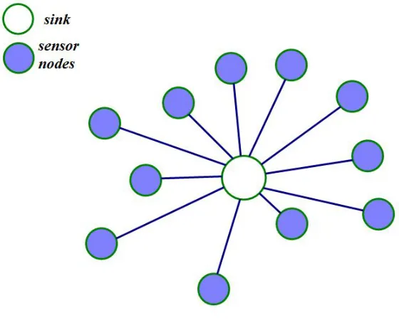
In this thesis we consider data storage systems that store in a single base station (that we call the sink) data collected from sensors. These systems might not be very efficient because some sensors might be far away from the base station and so it is expensive to send their data to the sink. An example of this kind of system is shown in Figure 1.1.

Figure 1.1: Example of a sensor network without storage nodes.

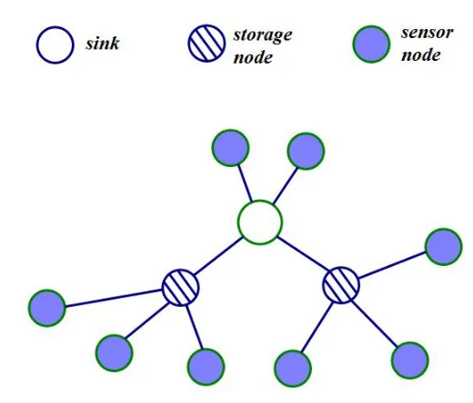
A more efficient system is one in which some sensors are designated asstorage nodeswhich can collect data received from adjacent sensors. A storage node is an enhanced version of a sensor node. It can also generate data and has much larger storage space and a bigger power source than the sensor nodes. Each sensor sends the information that it collects to a storage node and storage nodes send a summary of the information collected from the sensors to the sink node. This way the total amount of information sent to the sink is much smaller than the total amount of information that the storage nodes receive.

Storage nodes have a higher cost than sensor nodes as they need to provide storage for the data that they collect. We assume then that there is a limited numberk of storage nodes and that storage nodes have limited capacity, so that at most M sensors can send data to the same storage node, for some value M > 0. The problem that we consider in this thesis is given a wireless sensor network, select a set of at mostknodes to be designated as storage nodes that minimizes the cost of collecting the data from the sensor nodes and sending it to the sink. We call this problem the capacitated data storage placement problem (CDSP). A formal definition of the problem follows. LetN denote the number of sensor nodes including the sink. The sink is denoted as node 0. For each sensori∈N we define a variable

yi =

      

(6)

3

For each pairi, jof sensors (icould be equal to j) we define a variable:

xi j =

      

1 ifyi = 1 and sensor node jsends its data to storage nodei

0 otherwise

Figure 1.2: Example of a sensor network with storage nodes.

We useci j to denote the distance between nodesiand jand letδi be the distance between

nodeiand the sink. The distance between two nodes might be the Euclidean distance or any other metric. The cost or energy used by node jto send data of sizedto nodeiisci j∗d.

The capacitated data storage placement (CDSP) problem can be formulated as the following integer program:

IP:

min X

i,j∈N

xi j(α1ci j +α2δi)

s.t.X

i∈N

xi j =1,∀j∈N,

X

i∈N

yi ≤k,

X

j∈N

xi j ≤ Myi,∀i∈N

xi j ≤ yi,∀i, j∈N

y0 =1,yi,xi j ∈ {0,1}, ∀i, j∈N. (1.1)

In this integer program, α1is the total size of the data transferred between a sensor node and

(7)

that a storage node needs to send to the sink. For determiningα1andα2, we assume that each

node generates rg readings per unit of time, and the data size of each reading is sr. Also we assume there are rq queries per unit of time and σ is the ratio between the raw data and the compressed data that a sensor node sends to the sink. Then α1 = rgsr and α2 = rqσsr. The

objective function aims to minimize the total cost of transmitting information, which is equal to the sum of the cost of sending information from sensor nodes to storage nodes and the cost of sending information from storage nodes to the sink.

The first constraint, P

i∈Nxi j = 1,∀j ∈ N guarantees that each sensor node is assigned to

a storage node. If node jis assigned to storage node i, then xi j = 1 and for all other storage nodesh, xh j = 0. If xi j = 1 then sensor node j sends its data to storage nodei. The second constraint,P

i∈Nyi ≤ kensures that at mostkstorage nodes are selected. Each selected storage

nodeihasyi = 1. The third constraint,P

j∈Nxi j ≤ Myiensures that the total number of sensor

nodes assigned to a storage node is at mostM. This constraint is required because each storage node has limited capacityM. We also require that xi j ≤ yi, which means ifihas been chosen as a storage node, thenyi must be 1 and xi j could be 0 (sensor node jnot assigned to i) or 1 (sensor node jassigned toi); however, ifiis not a storage node then the value ofxi j cannot be 1. The last constraint,y0 = 1, guarantees that the sink is a storage node.

There is a well known optimization problem that is a special case of the CDSP problem called thek-median problem, which can be formulated as the following integer program:

IP:

min X

i,j∈N xi jci j

s.t.X

i∈N

xi j = 1,∀j∈N,

X

i∈N

yi ≤ k,

X

j∈N

xi j ≤ Myi,∀i∈N

xi j ≤yi,∀i, j∈N

yi,xi j ∈ {0,1}, ∀i, j∈N. (1.2)

(8)

5

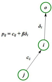
Figure 1.3: Definition of pi j.

The k-median problem and the capacitated k-median problem are known to be NP-hard. A problem His NP-hard if every decision problem in NP can be reduced in polynomial time to H [55]. If a problem is NP-hard, it is very unlikely that there exists a polynomial time al-gorithm for solving it as if such an alal-gorithm existed then polynomial time alal-gorithms would exist for all problems in NP. Hence, in this thesis we will concentrate on the design of ap-proximation algorithms for the capacitated data storage placement problem. An apap-proximation algorithm is an algorithms that can find approximate solutions to an optimization problem in polynomial time. Approximation algorithms are often used to deal with NP-hard problems, for which existing exact polynomial-time algorithms are too slow. Theapproximation ratioof an approximation algorithmAfor a problemH is the maximum ratiomax{_OPTS OL, OPT_{S OL}}of the value

S OLof the solution produced by the algorithmAfor any instance Iof problemH to the value

OPT of an optimum solution forI.

For the CDSP problem, depending on the values ofα1andα2, the first term,Pi,j∈Nα1ci jxi j,

or the second term,P

i,j∈Nα2xi jδi, in the objective function might be the dominant term. If α1

is much larger than α2, then the optimum solution will select a set of storage nodes that are

close to the sensor nodes. Otherwise, ifα2 is much larger thanα1, then the optimum solution

will select a set of storage nodes close to the sink. In general, we wish to find a set of storage nodes that are close to both the sensor nodes and the sink. For simplicity of notation we define

pi j = ci j+βδi as the local cost, whereβ = α_α2

1 and 0< β <1, so we can simplify the objective

function in the integer program (1.1) to minP

i,j∈Nxi jpi j.

We consider in this thesis the case when the distance function ci j satisfies the triangle in-equality [37]. The triangle inin-equality states that for any three nodes,h,i, j,ci j+cjh ≥cih. Note

that the cost function pi j does not necessarily satisfy the triangle inequality even if ci j does. Furthermore, pi j might not be symmetric as pi j =ci j+βδi andpji =cji+βδj.

(9)

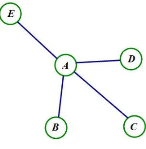
We can see from Figure 1.4 that nodesB,CandDare connected to the storage nodeAand

A is connected to the sink E. In this solution, A and E are selected as storage nodes, so the values of yA and yE are 1, and the value of yi for the other nodes is 0. Thus, the vectory is (1,0,0,0,1) (entries are in alphabetical order). xEA, xAB, xAC, xAD and xEE are all 1; all other variables xi jhave value zero. Thus, the matrixxis as follows:

                   

0 1 1 1 0 0 0 0 0 0 0 0 0 0 0 0 0 0 0 0 1 0 0 0 1

                   

In this thesis we present an approximation algorithm for the capacitated data storage placement problem in sensor networks with approximation ratio (16+23β+ 15₂β2_{), where}β = α2

α1. The

solution produced by our algorithm violates the capacity constraintsP

j∈Nxi j ≤ Myi by at most

a factor of 3, i.e. for any solution (x,y) produced by our algorithmP

j∈N xi j ≤3Myi, or in other

words the solution assumes that each storage node receives data from up to 3Msensor nodes.

Figure 1.4: A solution for the CDSP problem. NodesAandEare storage nodes.

Our algorithm first solves a modified integer program IP in which we allow variables yi

andxi j to take fractional values. Such a modification produces a so called linear program. The reason why we do this is that linear programs can be solved in polynomial time, but solving an integer program is NP-hard. The drawback of solving a linear program is that variablesyi and

xi j can have fractional values. So, for example ifyi = 1₂ andyj = 1₂ that means that nodesiand

jare ”half” storage nodes. Clearly such a solution, called afractional solution, does not make sense for our problem.

To transform a fractional solution into a valid solution for our problem (this latter solution is technically called an integer solution) we need to round the fractional values of the variables to integer values. Such a rounding causes the capacity constraint to be violated. If storage nodes have hard capacities (i.e. they can not be violated), we could initially set M0 = M

3 and

(10)

1.1. RelatedWork 7

1.1 Related Work

The data storage placement problem on sensor networks was proposed by Sheng et al. [49]. They assumed that sensor nodes have unlimited capacity, or in other words, that a storage node can receive information from an arbitrary number of sensor nodes and presented an approx-imation algorithm for the problem with approxapprox-imation ratio 10. In this thesis, we show that an algorithm by Arya et al. [5] can be used to solve the problem studied by Sheng et al. and the approximation ratio of the latter algorithm is only 5, greatly improving on the algorithm by Sheng et al.

The data storage placement problem is a generalization of the classicalk-median problem. In the k-median problem, the goal is to select a set S of k nodes from a graph G = (V,E) to be designated as centers, so that the sum of distances from the vertices in V \S to S is minimum [5, 13, 32, 33]. Thek-median problem has been extensively studied by the research community as it has a large number of applications in many areas like networks [36], data mining [43] and the web [46].

In the metric k-median problem, the distance function on the edges of the input graph G

satisfies the triangle inequality. Lin and Vitter proposed an approximation algorithm for the

k-median problem with approximation ratio 1+εfor any valueε >0, but that selects a set of (1+1_ε)(ln(n)+1)knodes as centers, wherenis the number of nodes in the graph [41]. The first approximation algorithm with constant approximation ratio for the metric k-median problem was proposed by Charikar, Guha, Shmoys and Tardos and it has approximation ratio 62₃ [13]. The algorithm is based on the solution of a linear programming relaxation of the problem and a complicated rounding procedure. Jain and Vazirani [32] improved on that algorithm by proposing an elegant algorithm based on primal-dual linear programming with approximation ratio 6 and running time O(mlogm(L + log(n))) where m is the number of edges, n is the number of vertices, and L = log₂dmax, wheredmax is the maximum length of the edges of the input graph. A primal dual approximation algorithm iteratively modifies two solutions: one for the linear program and one for its dual. A local search algorithm by Arya et al. [5] for the metric

k-median problem is the currently best algorithm for the problem and it has approximation ratio 3+2_pfor any integerp>0. Local search algorithms move from solution to solution in the space of candidate solutions (the search space) by applying local changes, until a solution deemed optimal is found.

A widely studied problem that is very related to thek-median problem is the facility location problem. Here we are given costs fi ≥0 for opening facilities. The problem is to select a subset of facilities to serve a group of clients such that the total facility cost plus the total service cost is minimized. The facility location problem is similar to thek-median problem except for the cost for opening the facilities. Thus, much of the research done on thek-median problem also considers the facility location problem. The facility location problem has many applications in operations research [20, 39], in network design problems such as placement of routers and caches [24,40], agglomeration of traffic or data [4,25], and web server replications in a content distribution network [34,46]. In the last decade this problem has been studied extensively from the perspective of approximation algorithms [14, 18, 19, 23, 38, 50, 52].

(11)

The capacitated facility location problem limits the number of clients that can connect to one facility. Jain et al. [31] gave a 3-approximation algorithm for a capacitated version of the facility location problem using primal-dual programming. Arya et al. [5] also proposed a local search algorithm for the capacitated facility location problem with approximation ratio 3.732+for any >0. When we set a capacity for each facility in thek-median problem, the problem is called the capacitatedk-median problem. Charikar [15] presented an approximation algorithm for the capacitatedk-median problem with approximation ratio 16; There is also a greedy algorithm by Mahdian et al [30] with approximation ratio 1.61 for the uncapacitated

k-median problem.

1.2 Our Contributions

In this thesis we study a local search algorithm for thek-median problem by Arya et al. [5] and show that we can use it to approximately solve the uncapacitated data storage placement prob-lem. We show that this algorithm has approximation ratio 5, greatly improving the algorithm by Sheng et al. which has approximation ratio 10.

(12)

Chapter 2 Local Search Algorithm for the

Uncapacitated Data Storage Placement

Problem

2.1 The Local Search Algorithm

We first would like to mention that in the nomenclature commonly employed with thek-median and facility location problems, storage nodes are called centers and sensor nodes are called clients. In this chapter we show that the local search algorithm in [5] for thek-median problem can be used to solve the uncapacitated data storage placement problem.

The algorithm first selects as initial solution S any set ofksensors. Then the solutionS is repeatedly modified by performingswap operations. In a swap operation, a storage node from

S is swapped with a node not inS; if the new solution has a cost smaller thanS, then the new solution is kept. Formally, the swap operation is defined as follows:

swap< s,s0 >:= S − s+s0fors∈Sands0 <S.

The algorithm is shown below.

Algorithm 1Local-Search (G,k) Input: GraphG =(V,E) and valuek.

Output: A set ofknodes to be used as storage nodes. 1. S ←an arbitrary set ofknodes fromG

2. While there is a swap operation< s,s0>such that cost(S − s+s0)<cost(S) do

S ←S − s+ s0

3. returnS

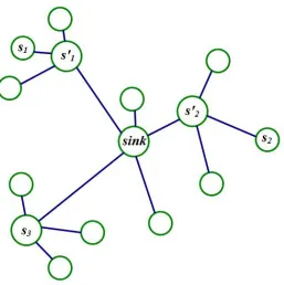
In Algorithm 1, cost(S) denotes the sum of all the local costs pi j defined in Chapter 1. Through the execution of the algorithm, there must be a time when we can not find two nodes to swap so thatcost(S − s+s0) <cost(S); at that moment, the algorithm ends and returns the solutionS. For an example, consider the instance shown in Figure 2.1 wherek = 4. Initially the algorithm selects S = {s1,s2,s3,sink}. The algorithm first considers the swap < s1,s0₁ >,

which yields a solutionS2 = {s01,s2,s3,sink}of lower cost, soS2is adopted overS1(see Figure

(13)

Figure 2.1: Solution S.

2.2). The swap< s2,s0₂ >then produces a solution S3 = {s0₁,s0₂,s3,sink}of smaller cost than

S2, soS3is taken as the current solution (see Figure 2.3). No swap can further reduce the cost,

soS3is a local optimum solution.

2.2 Analysis of the Local Search Algorithm for the

Uncapci-tated Data Storage Placement Problem

LetNS(s) denote the set of sensor nodes that send their data to storage node s∈S in the local optimum solution produced by algorithm Local-Search and letNS∗(o) denote the set of sensor

nodes that send their data to storage nodeo∈S∗in an optimum solutionS∗. We now compare the costs of solutions S and S∗ to determine the quality of the solution computed by Local Search. In the sequel, if a sensor nodes0 sends data to storage nodes, we say thats serves s0. Sensor nodes and storage nodes will sometimes be called just nodes when the meaning is clear from the context.

SinceS is a local optimal solution, we know that any swap< s,o>involving two different nodess∈S ando∈S ∗ \S is such that

cost(S −s+o)≥cost(S) (2.1)

For any nodes s∈S ando∈S∗we define ps = NS∗(o)∩NS(s) as the set of sensor nodes that

are served by, both, sin the local optimum solution andoin the optimum solution.

(14)

2.2. Analysis of theLocalSearchAlgorithm for theUncapcitatedDataStoragePlacementProblem11

Figure 2.2: SolutionS2.

(15)

Figure 2.4: SolutionS1.

Consider a 1-1 and onto mappingπ : NS∗(o)→ NS∗(o) with the property that for alls∈S such

that|ps| ≤ 1₂|NS∗(o)|, π(ps)Tps = ∅. To see how to build the mappingπ, the reader is referred

to [5].

We say that a storage nodeo∈S∗iscapturedby a storage node s∈S if|NS(s)T

NS∗(o)|>

1

2|NS∗(o)|. We call a storage node s ∈ S, bad if it captures at least one storage node in S∗

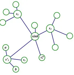
andgoodotherwise. To clarify these concepts consider the example shown in Figures 2.4 and 2.5. The optimum solution S∗ = {s1,s2,s3} for this example is shown in Figure 2.5 and a

(non-optimum) solution S1 = {s1, s2, s0₃} is shown in Figure 2.4. There are four nodes that

send data to storage node s3 in S∗: a, b, s0₃ and s3; also node s0₃ receives data from four

nodes in solution S1: a, b, s3 and s0₃. Thus, we say that s0₃ captures s3 because it satisfies

|NS1(s

0

3)

T

NS∗(s3)|> 1₂|NS∗(s3)|and hence s0₃is abadstorage node.

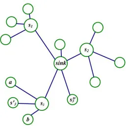
Consider now the solutionS4shown in Figure 2.6. Nodes00₃ is agoodstorage node because

it does notcaptureany storage nodes inS∗as|NS₄(s00₃)T

NS∗(s3)| = {b,s3}, so the number of

sensor nodes that send information to s00₃ is just half of the number of nodes inNS∗(s3).

To compare the cost of the solution S computed by the local search algorithm with the cost of an optimum solution S∗, we consider the following set ofk swap operations< s,o >

between storage nodes inS and storage nodes inS∗:

1. If s is a bad storage node that captures only one storage nodeo ∈ S∗, we consider the

swap< s,o>.

2. Bad storage nodes capturing at least 2 storage nodes fromS∗will not be swapped. 3. Each good storage node inS is swapped with a storage node inS∗which is not

(16)

Figure 2.5: Optimum SolutionS∗.

(17)

storage nodes inS capturing at least 2 nodes ofS∗are not swapped, then the number of good storage nodes inS is at least half of the number of storage nodes inS∗which are not considered in step 1.

Note that in the above set of swap operations, if a swap< s,o>is considered, the storage node

sdoes not capture any node o0 ∈ S∗, o0 _, o. When a swap < s,o > operation is considered we need to reassign the sensor nodes inNS(s)∪NS∗(o) to the storage nodes inS −s+o. After

we perform the swap operation< s,o>all sensor nodes j∈NS∗(o) are assigned tooand each

sensor node jis assigned to the storage nodesj ∈S −s+ofor which psjjis minimum.

Figure 2.7: Reassigning the nodes inNS(s)∪NS∗(o).

Consider a node j0 ∈ NS(s)∩NS∗(o0), foro0 _, o. As sdoes not captureo0, then|NS(s)∩

NS∗(o0)| ≤ 1₂|NS∗(o0)|and by the way in which mappingπhas been defined, we have thatπ(j0)<

NS(s). So letπ(j0₎_∈_NS₍_s0_{). Note that the cost of assigning} _j0 _{to a storage node in}_S ₋_s+_o_is

at mostcj0_s0 (see Figure 2.7). Since storage nodes need to forward information to the sink, as

explained in Chapter 1, the cost function in which we are interested isps0_j0 =cs0_j0+βδ_s0, which

indicates that the communication cost between s0 _and _j0 _{is equal to the cost of transmitting}

information from node j0 to the storage node s0 plus the cost of sending information from the storage node s0 to the sink. So let us analyzeps0_j0.

(18)

Proof We know that by the triangle inequality,cs0_j0 ≤cs0_π₍_j0₎+co0_π₍_j0₎+co0_j0, then ps0_j0 =cs0_j0 +βδ_s0 ≤co0_j0 +co0_π₍_j0₎+cs0_π₍_j0₎+βδ_s0

≤ co0_j0+co0_π₍_j0₎+ ps0_π₍_j0₎

≤ co0_j0+co0_π₍_j0₎+ ps0_π₍_j0₎+(2βδ_o0−2βδ_o0)

= co0_j0+βδ_o0 +co0_π₍_j0₎+βδ_o0+ ps0_π₍_j0₎−2βδ_o0

= po0_j0 +po0_π₍_j0₎+ ps0_π₍_j0₎−2βδ_o0

Figure 2.8: Relationship between the nodes in Lemma 2.2.1.

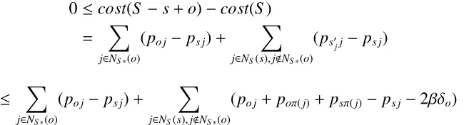
We can now comparecost(S) andcost(S∗). First, by inequality (2.1),

0≤cost(S −s+o)−cost(S)

= X

j∈NS∗(o)

(po j− ps j)+ X

j∈NS(s),j<NS∗(o)

(ps0

jj− ps j)

≤ X

j∈NS∗(o)

(po j− ps j)+ X

j∈NS(s),j<NS∗(o)

(po j+ poπ(j)+psπ(j)−ps j−2βδo) (2.2)

where the last inequality follows from Lemma 2.2.1.

Inequality (2.2) holds for each swap operation < s,o > where s ∈ S and o ∈ S∗. If we consider the set ofkswap operations described above, then note that each storage node s ∈S

participates in at most two swaps; hence the last term in inequality (2.2) added over allkswaps is at most 2P

(19)

the information from sensor node jin the optimum solutionS∗andsj is the storage node that

collects information from node jin solutionS.

Sinceπis a 1−1 and onto mapping, then each node jis mapped to a unique nodeπ(j) and so

X

j∈N pojj =

X

j∈N

pojπ(j) =cost(S∗). Similarly,P

j∈N psjj =

P

j∈N psjπ(j). Therefore, by the above equation 2X

j∈N

(po_jj+ pojπ(j)+ psjπ(j)−psjj−2βδo)=4cost(S∗)−4β

X

j∈C

δoj.

By inequality 2.2 added over allkswap operations, we get:

0≤ X

j∈N

(pojj− psjj)+

X

j∈N

(pojj+ pojπ(j)+psjπ(j)− psjj−2βδoj) ≤ cost(S∗)−cost(S)+4cost(S∗)−4X

j∈N

βδoj.

≤ 5cost(S∗)−cost(S) (2.1)

Hence:cost(S)≤ 5cost(S∗)

(20)

Chapter 3 Approximation Algorithm for the

Capacitated Data Storage Placement

Problem

3.1 Outline of the Algorithm

In the linear program relaxation of an integer program the requirement that the variables take only integer values is relaxed by allowing them to take real values. We will consider a more general version of integer program (1.1) by allowing each node j to have a non-negative de-manddj. This demand can be regarded as the importance of the node or the size of the data that it generates. We will use this more general formulation of the problem as it is more convenient for expressing and analyzing our algorithm. The linear programming relaxation of this more general version of (1.1) is the following:

min X

i,j∈N

djpi jxi j

s.t.X

i∈N

xi j =1,∀j∈N,

X

i∈N

yi ≤k,

X

j∈N

djxi j ≤ Myi,∀i∈N

yi ≥ xi j ≥0,∀i, j∈N,y0= 1 (3.1)

In the data storage placement problem, the demand dj is set to 1 for all nodes j. However, later to analyze the algorithm we will modify the demands of the nodes and that is why we have added the terms dj to the objective function. Recall that pi j is neither symmetric (i.e. pi j = ci j +βδi is not necessarily equal to pji = cji + βδj) nor proportional to the Euclidean

distance betweeniand j, as pi j =ci j+βδi.

The steps of our algorithm for the capacitated data storage placement problem are outlined below. Each step is analyzed in detail in the following sections.

(21)

Step 1: Compute a solution ( ¯x,y¯) for the linear program (3.1). Let ¯Cp_j indicate the cost of processing the information generated by sensor node jin solution ( ¯x,y¯); i.e.

¯

Cp_j =X i∈N

pi jxi j¯

Then the value of the solution ( ¯x,y¯) can be written as:

¯

CLP( ¯x,y¯)=X

j∈N djC¯

p j

Next we find a setN0 of nodes that satisfies the following two properties.

• For all j∈N−N0there existsi∈N0such thatci j ≤4 ¯Cp_j.

• For alli, j∈N0,ci j >4max{C¯_ip,C¯p_j}.

We call N0 _{the set of}_{core nodes}_{. For every core node}_i _in_N0 _{there is a radius 2 ¯}_Cp

i such that

every node j ∈ N−N0 within this radius is closer toithan to any other core node (see Figure 3.1).

Figure 3.1: Core nodes.

To understand the notion of core nodes, consider the example in Figure 3.1. From the above figure we can see thatci1i2 is larger than 4max{C¯

p i1,

¯

C_ip

(22)

3.2. Step1: IdentifyingCoreNodes 19

property. Node j1 ∈N−N0is no more than 4 ¯C

p

i1 away fromi1, so j1satisfies the first property.

On the other hand, node j2 ∈ N− N0 is not within the 4 ¯C

p

i1 radius ofi1, but it must be within

that distance from other core node. Additionally, j3is within the 2 ¯C

p

i2 radius ofi2, so it is closer

toi2 than to any other core node.

Step 2: Modify the solution ( ¯x,y¯) computed in Step 1 by combining fractional values (a value zis called fractional if it is not integer) ¯xi j and ¯yi to obtain a new solution (x0,_y0_{) with}

fewer variables with positive values. A nodei∈N−N0is called afractional centerif ¯yi is not integer. Each fractional center is assigned to the closest node inN0 (breaking ties arbitrarily). For every fractional centeriwe consider the set of sensor nodes assigned to it and redistribute them among nodeiand the node in N0 closest to it so that every variabley0_i has value at least

1

2. Note that the solution created in this manner could violate the capacity constraints because

too many sensor nodes could be assigned to a storage node.

Step 3: Further modify the solution obtained in the previous step to produce a {1/2, 1} -integral solution for the linear program. In a{1/2, 1}-integral solution, all variables have value 0,1₂ or 1.

Step 4: Convert the{1/2,1}-integral solution into an integral solution ( ˆx,yˆ) with at most a factor 3 increase in the capacities. In the next sections we explain in detail each step of the algorithm.

3.2 Step 1: Identifying Core Nodes

We first compute a solution ( ¯x,y¯) for the linear program (3.1) using the Ellipsoid algorithm [1, 8] and identify a set N0 of core nodes in the following manner. Initially, N0 = φ; let

N = {1, . . . ,n} be the set of nodes indexed in increasing order of ¯Cp_j, i.e. C¯₁p ≤ · · · ≤ C¯np.

Consider the nodes j =1, . . . ,nin this order. For each node j, if there is no nodei < j,i ∈N0

for whichci j ≤ 4 ¯Cp_j, then add jtoN0. For a node j∈N, letl(j) denote the closest node to jin

N0 breaking ties arbitrarily.

Corollary 3.2.1 cl(j)j ≤4 ¯C p j

Proof Because of the way in which the set N0_{is chosen, for any node} _j_∈_N_,_cl

(j)j ≤4 ¯C p

j.

For each nodei ∈ N0 we define Mi as the set of nodes in N closer toithan to any other node inN0, i.e. Mi = {j∈N :l(j)= i}. We define thefractional center valueof Miaszi = P

j∈Miyj. Since for anyi,h∈N0_,_cih >_{4 ¯}_Cp

i, then each node j∈N within a 2 ¯C p

i radius ofi ∈N

0 _{must be}

closer toithan to any other node inN0and so it must belong toMi. Note that for any node j∈ N, ¯Cp_j = P

i∈Npi jxi j¯ can be regarded as the weighted average of

the costs pi j, where ¯xi jis the weight of pi j. Since in any weighted average, less than half of the total weight can be given to values more than twice the average, then

X

i:pi j>2 ¯Cp_j ¯

xi j < 1

2 (3.2.1)

SinceP

i∈Nxi j¯ = 1 and ¯xi j ≤yi¯ for eachi∈N, then

X

i:pi j≤2 ¯Cpj ¯

yi ≥ X

i:pi j≤2 ¯Cpj ¯

xi j ≥ 1

(23)

Additionally, because pi j ≥ ci j, then

X

ci j≤2 ¯Cp_j ¯

yi ≥ X

pi j≤2 ¯Cp_j ¯

yi ≥ 1 2

Thus, for any feasible fractional solution ( ¯x,y¯) of linear program (3.1),P

i:ci j≤2 ¯Cp_j yi¯ ≥

1

2 for each

j∈N. Therefore, the total fractional center valueziof the setMi is greater than or equal to 1₂.

3.3 Step 2: Consolidating Storage Nodes

We modify the solution ( ¯x,y¯) by performing a series of transfer operations as indicated by the following algorithm.

Algorithm 2Transfer ( ¯x,¯y,Mi,i)

Input: Solution ( ¯x,y¯) of linear program (3.1), core nodeiand set of nodesMi. Output: Modified solution (x0,y0).

1. Initially, set (x0,y0)= ( ¯x,y¯). Sort the nodes jinMiin increasing order ofci j, i.e. if the sorted nodes are j1, j2, . . . , jm, thenci j1 ≤ci j2 ≤ · · · ≤ci jm.

2. Let jtbe the first node in the sequence j1, . . . , jmsuch thaty0jt <1. Let jsbe the first node in the sequence jt₊1, . . . , jmsuch thaty0js > 0. If either jsor jtdoes not exist, go to step 6.

3. q←min(y0_j

s,1−y

0

jt). 4. For all nodes j0∈N, set

x00jtj0 ← x

0

jtj0+

q y0_j

s

x0jsj0

x00jsj0 ← x

0

jsj0 −

q y0

js

x0jsj0

Sety00_j

t ←y

0

jt +q,y

00

js ←y

0

js −q. 5. For all j0 ∈N, setx0_j

tj0 ← x

00

jtj0, x

0

jsj0 ← x

00

jsj0,y

0

jt ←y

00

jt,y

0

js ←y

00

js and then go back to step 2. 6. If there is a node jt, 1<t≤ msuch that 0< y0_j

t <1, then we assign the demand served by jt to jt−1: For all nodes j0 ∈N, we set

x0_j

t−1j0 ← x

0

jt−1j0+ x

0

jtj0

x0jtj0 ←0

y0jt ←0

7. Return (x0,y0)

We now show that the solution (x00,_y00_{) computed in Step 4 of algorithm Transfer satisfies}

(24)

3.3. Step2: ConsolidatingStorageNodes 21

is satisfied for all j1, j2, . . . , jt−1 by induction hypothesis and the fact that ( ¯x,y¯) is a solution of

(3.1). To see that the constraint holds for js, note that

X

j0_∈_N

djx00jsj0 =

X

j0_∈_N

dj(x0jsj0−

q y0_j

s

x0jsj0)

= (1− q

y0

js )X

j0_∈_N djx0jsj0

≤ (1− q

y0

js

)Myj0_s by induction hypothesis

= M(y0_j

s −q)= My

00

js

A very similar argument shows that the constraint also holds for jt.

Step 6 of Transfer, however might increase the load of node jt−1to at most 2Mas the whole

load of node jt is transferred to jt−1.

To show how algorithm Transfer works, consider an instance where for core nodei, Mi =

{j1, j2, j3, j4, j5}, and suppose thaty0 = (2₃ 1₂ 1₃ 0 0); the valuesx0jijh for 1 ≤i,h≤ 5 are given by the following matrix:

                    2 3 1 2 1 2 2 3 1 2 1 3 1 2 1 3 0 1 2

0 0 1₆ 1₃ 0 0 0 0 0 0 0 0 0 0 0

                   

In this example, the sum of values in each column is 1. In the first execution of steps 2-5 algorithm Transfer sets jt = j1 and js = j2; the values iny0 change to (1 1₆ 1₃ 0 0). The matrix

x0becomes

                    8 9 5 6 13 18 2 3 5 6 1 9 1 6 1 9 0 1 6

0 0 1₆ 1₃ 0 0 0 0 0 0 0 0 0 0 0

                   

because part of the load from the nodes assigned to j2 is now transferred to j1. In the second

execution of steps 2-5 the algorithm chooses jt = j2 and js = j3. The new vectory0 is y0 =

(1 1₂ 0 0 0) and x0_is

                    8 9 5 6 13 18 2 3 5 6 1 9 1 6 5 18 1 3 1 6

0 0 0 0 0 0 0 0 0 0 0 0 0 0 0

                   

Since the value ofy0_j

2 is greater than 0 and less than 1, step 6 is executed to produce the final

solutiony0 = _{(1 0 0 0 0) and}

x0 =

                   

1 1 1 1 1 0 0 0 0 0 0 0 0 0 0 0 0 0 0 0 0 0 0 0 0

(25)

Note thaty0_j

2 =0 which means this node will not receive message from any other nodes and so

the load of node j2is transferred to j1; the load of j1increases to at most 2M.

In step 4, variable x0

jsj0 is combined with x

0

jtj0. We say that x

0

jsj0 is terminally modified to node jt in step 4 if and only if zl(js) =

P

i∈Ml(js)y

0

i ≥ 1, otherwise, the variable is said to be non-terminally modified. The reason we call these variables terminally modified and non-terminally modified is because ifzl(js) ≥ 1, then the valuesy

0

i of the nodesiinMl(js)can be transferred to

l(js) sol(js) will be one of the chosen storage nodes and so sensor node jswill be ”terminally” assigned tol(js); otherwise, nodes in Ml(js)do not accumulate enough valuezl(js) and thusl(js) will not be a storage node, so the sensor nodes in Ml(js) will be assigned to other nodes. The following two lemmas bound the cost of the solution produced by algorithm Transfer.

Lemma 3.3.1 For variable x_{i j}0 > 0terminally modified to nodei0 ∈ Ml(i), pi0_j ≤ (3+2β)pi j +

8(1+β) ¯Cp_j.

Proof By Steps 1 and 2 of algorithm Transfer, i0_{must appear before}_i_{in the ordering of}_Ml

(i),

thus,

cl(i)i0 ≤ cl₍_i₎_i. (3.3.1)

Since for any node j∈N, pi0_j =ci0_j+βδ_i0 andδ_i0 = coi0, whereois the sink, then by the triangle

inequality (see Figure 3.2),

pi0_j =ci0_j+βδ_i0 ≤ci0_l₍_i₎+cl₍_i₎_i+ci j +β(δ_i+ci0_i)

≤2cl(i)i+ci j+β(δi+ci0_l₍_i₎+cl₍_i₎_i), by inequality (3.3.1) and the triangle inequality

≤2cl(i)i+ci j+β(δi+2cl(i)i), by inequality (3.3.1)

≤2(1+β)cl(j)i+ci j+βδi, asiis closer tol(i) than tol(j)

≤2(1+β)(cl(j)j+ci j)+ci j+βδi, by the triangle inequality

=2(1+β)cl(j)j+(3+2β)ci j+βδi

≤2(1+β)cl(j)j+(3+2β)pi j

≤2(1+β)pl(j)j+(3+2β)pi j, as pl(j)j ≥cl(j)j

≤8(1+β) ¯Cp_j +(3+2β)pi j, by Corollary 3.2.1

Lemma 3.3.2 For variablexi j¯ > 0non-terminally modified to l(i), we have pl(i)j ≤ (2+β)pi j+

4(1+β) ¯Cp_j.

Proof By the triangle inequality: cl(j)i ≤ ci j +cl(j)j and cl(i)j ≤ ci j +cl(i)i ≤ ci j +cl(j)i because iis closer to l(i) than tol(j). Combining these two inequalities we getcl(i)j ≤ 2ci j +cl(j)j. In

addition,βδl(i)≤ β(cl(i)i+δi)≤β(cl(j)i+δi)≤ β(ci j+cl(j)j+δi) by the triangle inequality. Thus, pl(i)j = cl(i)j+βδl(i) ≤ 2ci j +cl(j)j+βci j +βcl(j)j+βδi ≤ (2+β)pi j +4(1+β) ¯C

p

j by Corollary

3.2.1.

We define the modified demandd_i0of a core nodei∈N0as follows.

d0_i ← X

j∈N djx0i j

(26)

3.4. Step3: Obtaining a n₁

2,1

o

-IntegralSolution 23

Figure 3.2: Relationship between the nodes in the proof of Lemma 3.3.1.

3.4 Step 3: Obtaining a

n

1₂

,

1 o

-Integral Solution

We now define two new sets of nodes: N1 =

n

i∈N :y0_i > 0o and N2 =

n

i∈N : 0<y0_i <1o. Note that according to algorithm Transfer the only nodes that belong to N2 are those core

nodesi0 _∈ _N0_{for which}_y0

i < 1 andy

0

j = 0 for all j ∈ Mi. Therefore,N2 is a subset ofN

0_{. Let}

|N1|= `and|N2|=m.

Lemma 3.4.1 For each node i∈N2, y0i ≥

1 2.

Proof Sinceiis a core node andy0_j =0 for all j∈Miexcepti, thenicollects all the information sent by the nodes in Mi. By the discussion at the end of Section 3.2,

1 2 ≤zi =

X

j∈Mi

y0j =y

0

i

To obtain an1₂,1o-integral solution ( ˆx,yˆ) from the solution (x0,y0) computed by algorithm Trans-fer we first set ˆyj ← 1 for all nodes j∈N1−N2. We sort the nodes jinN2in increasing order

of valued0_jps(j)j: let these nodes be j1, . . . , jm. We give the first 2(` −k) nodes jin this order

value ˆyj = 1₂ and for the rest we set ˆyj = 1. We also sort the nodes in N1 in the same above

order. For each node j ∈N2, let s(j) be the node inN1− {j}that has the minimum value ps(j)j

breaking ties in favor of a node with smaller index.

Observe that the new solution (x0,yˆ) could be infeasible because the last constraint,

ˆ

(27)

of linear program (3.1) might not be satisfied as some values ˆyj are smaller than the

corre-sponding valuesy0_j.

The following lemma shows that for every nodeiwith value ˆyi = 1₂ the total demand served by it is at mostM.

Lemma 3.4.2 For any node i,

1. Ifyiˆ = 1₂, thenP

j∈Ndjx0i j ≤ M. 2. Ifyiˆ = 1, thenP

j∈Ndjx_{i j}0 ≤2M.

Proof The only nodesiwith value ˆyi = 1₂ belong to N2, i.e. core nodes for whichy0 < 1 and

y0

j = 0 for all j ∈ Mi. Algorithm Transfer does not change the value y

0

i for these nodes and

so by the third constraint of linear program (3.1), P

j∈Ndjx

0

i j ≤ My

0

i ≤ M. The last step of

algorithm Transfer might change the values of some variablesy0_i so that 1 < y0_i < 2. For such variables y0

i the value of the corresponding variable ˆyi is 1. By the third constraint of linear

program (3.1),P

j∈Ndjx

0

i j ≤ My

0

i <2M. Finally, for those variablesy

0

i that have value 1, ˆyi = 1

andP

j∈Ndjx0_{i j} ≤ My0_i ≤ M <2M.

The following lemma will help us bound the total cost of our solution.

Lemma 3.4.3

X

i∈N2

(1−yiˆ)di0ps(i)i ≤

X

i∈N2

(1−y0i)d

0

ips(i)i .

Proof Note that

X

i∈N1

(1−y0i)d

0

ips(i)i =

X

i∈N2

(1−y0i)d

0

ips(i)i+

X

i∈N1−N2

(1−y0i)d

0

ips(i)i =

X

i∈N2

(1−y0i)d

0

ips(i)i

because y0_i = 1 for all i ∈ N1− N2. Hence, to prove the lemma we only need to show that

the function f(y1,y2, . . . ,y`)=Pi∈N1(1−yj)dips(i)ihas its minimum value wheny1,y2, . . . ,y` =

ˆ

y1,yˆ2, . . . ,yˆ` given thatyi ≥ 1₂ for alli=1,2, . . . , `.

Since the variablesyi are indexed in non-decreasing order ofdips(i)i, anddips(i)i > 0 for all i=1,2, . . . , `, function f will have its minimum value when the first variablesyi(with smallest

dips(i)ivalue) have value 1₂ and the last variablesyi(with largedips(i)ivalue) have value 1. Since

by the second constraint of linear program (3.1),P

i∈N1yi = k, then the minimum is achieved

when the first 2(`−k) variables have value 1₂ and the remaining ones have value 1. Note that with this assignment of values to the variablesyi,

X

i∈N1

yi = 1

22(`−k)+`−(2(`−k))

=`−k+`−2`+2k =k as required.

(28)

3.5. Step4: Rounding to anIntegralSolution 25

3.5 Step 4: Rounding to an Integral Solution

The last step of the algorithm transforms the solution (x0,_y_ˆ_{) into an integral solution. To do this}

we first build a directed graph as follows. Create a node for eachi ∈N1. For eachi∈ N2with

ˆ

yi = 1₂, add a directed edge fromitos(i); see Figure 3.3.

Figure 3.3: Directed graph induced bys(j).

Note that because of the way in which s(i) is chosen for a node i, the only cycles in this directed graph are formed by pairs of vertices (i, j) such that s(i)= jands(j)=i.

For each cycle, we designate one of the vertices as a root node and delete the edge directed from the root to the other vertex to form a tree. If the directed graph has several components, this process transforms the graph into a collection of trees. In the figure, we can see that the edges between nodes j1 and j2 form a cycle. We choose j1 as root and remove the edge from

j1to j2 (see Figure 3.4). Observe that the nodes with only directed edges pointing to them are

(29)

Figure 3.4: Converting the directed graph into a tree.

The above process produces a collection of rooted trees spanning the nodesi∈N2with ˆyi = 1

2. In the solution (x

0_,

ˆ

y) we choose all the nodes iwith ˆyi = 1 as storage nodes. Additionally, we will choose half of the nodesiwith ˆyi = 1₂ as storage nodes as described below.

We define thelevelof a node in a tree to be the number of edges on the path from the node to the root of the tree. Consider any treeT in the collection. We decomposeT into a collection of stars that will be used to select the nodes that will be chosen as storage nodes. Start from a leaf nodeiofT of highest level and remove the subtree rooted at its parents(i). This creates a star rooted at s(i). Repeat this procedure until the tree is empty or it consists of a single nodei. In the latter case, if ˆyi = 1₂, we addito the star rooted at s(i). Recall that s(i) is the node that has the minimum value ps(i)i inN1− {i}. The figure below shows how to split a tree into stars

for the above example.

(30)

Definition A star is calledevenif the sum of the ˆyi values of the nodesiin the star is integer. A star that is not an even star is called anoddstar.

To determine which of the nodes in a star is going to be selected as a storage node, we need to consider 4 cases depending on whether the star is even or odd and whether the rootiof the star has value ˆyi =1 or ˆyi = 1₂. For each one of these cases we will consider two different selections of storage nodes. At the end we will choose either the selection of storage nodes of smaller cost or the selection with smaller number of nodes, as explained later.

In all cases the rootiof a star is selected as a storage node.

1. Even star rooted at a nodeiwith ˆyi =1. Let j1, . . . , j2rbe the children ofiin non-decreasing

order of pi jk. Note that since the star is even and ˆyi = 1 then the number of children of i must be even. We consider the two following selections of storage nodes.

a) Select j1, j3, . . . , j2r−1 as storage nodes. Node j2s is assigned to node j2s−1 for each

s=1,2, . . . ,r, which means that the demand of j2sis transferred to j2s−1. To reflect this

fact the variables x0 _{need to be updated: For each node}_i _∈ _N_{, set}_x0

j2s−1i ← x

0

j2s−1i+ x

0

j2si andx0_j

2si ←0. In the sequel we will not explicitly indicate how the values of the variables

x0 are updated. For this case, nodes j2s−1,s = 1,2, . . . ,r, have demand at most 2M by

Lemma 3.4.2. By the same lemma the demand of nodeiis at most 2M.

Figure 3.6: Case (1), selection (a).

b) Select nodes j2, j4, . . . , j2r as storage nodes. Node j1 is assigned to the rootiand node

j2s+1 is assigned to j2sfor all s=1,2, . . . ,r−1. By Lemma 3.4.2 the rootihas demand

at most 2Mbecause ˆyi =1; hence, its demand becomes at most 3Mafter assigning j1to

(31)

Figure 3.7: Case (1), selection (b).

2. Even star rooted at a node i with ˆyi = 1₂. Let j1, . . . , j2r+1 be the children of i in

non-decreasing order of pi jk

a) Select nodes j2, j4, . . . , j2r as storage nodes. Node j1 is assigned to the rootiand node

j2s+1 is assigned to node j2s for all s = 1,2, . . . ,r; this will cause the demand of the

storage nodes to increase to at most 2M.

b) Select nodes j3, j5, . . . , j2r+1as storage nodes. Nodes j1and j2 are assigned to the rooti

and node j2s+2is assigned to j2s+1 fors = 1,2, . . . ,r−1. The rootiwill have a demand

(32)

3. Odd star rooted at nodeiwith ˆyi = 1. Let j1, . . . , j2r+1be the children ofiin non-decreasing

order of pi j_k.

a) Select nodes j2, j4, . . . , j2r, j2r+1as storage nodes. Node j1is assigned to the rooti. Node

j2s+1is assigned to j2sfor alls=1,2, . . . ,r−1. This will cause an increase in the demand

of some storage nodes to at most 2M. Since j1moved its demand to the root, the demand

for the root increased to at most 3M.

b) Select nodes j1, j3, j5, . . . , j2r−1as storage nodes. Node j2r+1is assigned to the rootiand

node j2sis assigned to j2s−1for alls=1,2, . . . ,r. From Lemma 3.4.2, the demand of the

rootiis 2Mand theniwill have a demand at most 3Mafter assigning j2r+1with demand

(33)

4. Odd star rooted atiwith ˆyi = 1₂. Let j1, . . . , j2r be the children ofiin non-decreasing order

of pi j_k.

a) Select nodes j2, j4, . . . , j2r as storage nodes. Node j1 is assigned to the root. Each node

j2s+1 is assigned to node j2sfor all s = 1,2, . . . ,r−1. In this case, some storage nodes

have a demand of at most 2M.

b) Select nodes j3, j5, . . . , j2r−1as storage nodes. Nodes j1and j2 are assigned to the rooti

and each one of the remaining even nodes j2sis assigned to node j2s−1. In this case, the

(34)

From the above discussion, we see that the demand for storage nodes can be increased to at most 3M.

Let r(i) be the storage node to which nodei was assigned in the above process. The cost of a selection S of storage nodes is defined to be P

i∈S d

0

ipr(i)i. For each even star we choose

the selection of storage nodes (a) or (b) of smaller cost. For odd stars we proceed as follows. Note that there is an even number of odd starsS1,S2, . . . ,S2q because the total sum of the ˆyi

variables must be integer. LetCa(`) denote the cost of starS`under selection (a) andCb(`) for

selection (b). We let the stars be numbered in increasing order of value|Ca(`)−Cb(`)|. We choose the lower cost selection forSq+1, . . . ,S2qand choose the selection with smaller number

of centers forS1, . . . ,Sq. Now we analyze the total cost of the stars.

Lemma 3.5.1 The total cost of the stars computed by the above procedure is bounded by the sum over all stars of the average cost of the two selections (a) and (b).

Proof For the even stars, we choose the selection of storage nodes of smaller cost, so their total cost is at most the sum of average costs of (a) and (b). For the odd stars, we need to be more careful, as we might choose the larger cost selection for some of them. Consider pairs of odd stars (S`,S2q−`+1) for` ≤ q; the worst case is when the cost forS`is the higher of (a) and

(b). Note that given two non-negative values f andg,

max(f,g)= 1

2|f −g|+ 1

2|f +g| and (3.5.1) min(f,g)= 1

2|f +g| − 1

2|f −g| (3.5.2) Thus, the cost for pair (S`,S2q−`+1) can be bounded by

min(Ca(2q−`+1),Cb(2q−`+1))+max(Ca(`),Cb(`))

= 1

2|Ca(2q−`+1)+Cb(2q−`+1)|+ 1

2|Ca(`)+Cb(`)|

+ 1

2|Ca(`)−Cb(`)| − 1

(35)

Consider the last two terms in the above expression. Because of the way in which the costs of the starsS` were ordered we know that

|Ca(`)−Cb(`)| ≤ |Ca(2q−`+1)−Cb(2q−`+1)|.

Thus,

min(Ca(2q−`+1),Cb(2q−`+1))+max(Ca(`),Cb(`)) ≤ 1

2|Ca(2q−`+1)+Cb(2q−`+1)|+ 1

2|Ca(`)+Cb(`)|

We now use the previous lemma to bound the cost of the stars chosen by the algorithm.

Lemma 3.5.2 The cost of the stars chosen by the algorithm can be bounded by(1+β₂)P

j∈N2,yˆj=12 d

0

jps(j)j.

Proof Recall that in a starS` all the children nodes jhave value ˆyj = 1₂. The cost of the root iofS`is zero asiis selected as a storage node. For the children nodes jwe need to consider

tree cases:

(1) In one of the selections (a) or (b), node jis chosen as a storage node (so its cost is zero) and in the other selection jis assigned to one of its siblings j0_{. In the latter case the cost of} _j_is

d0_jpj0_j.

(36)

Note that (see Figure 3.14)

pj0_j =c_j0_j+βδ_j0 ≤ cs₍_j₎_j+cs₍_j₎_j0+β(δ_s₍_j₎+cs₍_j₎_j0), by the triangle inequality

≤2cs(j)j+βcs(j)j+βδs(j), cs(j)j0 ≤cs₍_j₎_j by the way in which storage nodes are chosen

<(2+β)cs(j)j+βδs(j)

<(2+β)ps(j)j

Hence, the average cost of jis at most 1₂(0+(2+β)d0

jps(j)j)=(1+

β

2)d

0

jps(j)j.

(2) In one of the selections (a) or (b), jis chosen as a storage node and in the other it is assigned to the root. In the second case the cost of jisd0_jps(j)j.

(3) Node jis assigned to the root in both selections (a) and (b). The cost of jis thend0

jps(j)j.

In the three cases the average cost of jis at most (1+ β₂)d0_jps(j)j. By Lemma 3.5.1 the cost

of the stars is as stated.

We are now ready to bound the cost of the non-terminal assignments.

Lemma 3.5.3 In the solution provided by our algorithm, the cost of the non-terminal assign-ments increases by the cost of the stars, which is2(1+ β₂)P

j∈N2(1−y

0

j)d

0

jps(j)j.

Proof Recall that we have definedd0_j =P

j∈Ndjx0i j. Consider all the non-terminal assignments

from nodes jto nodei, that are re-assigned in the above procedure tor(i):

X

j

djx0i jpr(i)j =

X

j

djx0_{i j}cr(i)j+

X

j

djx0_{i j}βδr(i)

≤X

j

djx0i jcr(i)i+

X

j djx

0

i jci j+

X

j djx

0

i jβδr(i), by the triangle inequality

≤X

j

d0jpr(i)i+

X

j

djx0i jpi j

The first term of the right hand side of the last inequality is the cost of the stars and the second term is the cost of the non-terminal assignments before step 4. The nodes in the stars are all in

N0and for all the children nodes j,y0_j = 1₂, so using Lemma 3.5.2, the first term can be bounded by:

(1+ β 2)

X

j∈N2,yˆj=12

d0jps(j)j =(1+

β

2)

X

j∈N2

2(1−yjˆ )d0jps(j)j ≤(1+

β

2)

X

j∈N2

2(1−y0j)d

0

jps(j)j

(37)

Computing the Total Cost of the Solution

and the Time Complexity of the Algorithm

In this chapter we analyze the total cost of the solution for the data storage placement problem produced by our algorithm and compute its time complexity. We have proven some lemmas in the previous chapters that will help us compute the total cost of the solution.

4.1 Analyzing the Total Cost of the Solution

In Section 3.3 we computed a solution (x0,y0), and for some of the sensor nodes jwe produced terminally modified assignments xi j. These assignments are part of the final solution, i.e. if

xi j = 1 theni is a storage node in the final solution and sensor node j is assigned to it. For other sensor nodes j we produced non-terminally modified assignments. For such nodes the final selection of storage nodes to which they will be assigned is made in Section 3.4 and 3.5. To determine the total cost of the solution we need to compute the cost of the terminally and non-terminally modified assignments. The cost of the terminally modified assignments is given by Lemma 3.3.1:

X

j∈N

X

i:zl(i)≥1,i∈N0

((3+2β)pi j +8(1+β) ¯C_ip)djx0i j (4.1)

Computing the cost of the non-terminal assignments is more complicated. By Lemma 3.3.2 the cost of these assignments after step 2 is

X

j∈N

X

i:zl(i)<1

((2+β)pi j+4(1+β) ¯Cp_j)djx0i j (4.2)

(38)

4.1. Analyzing theTotalCost of theSolution 35

Steps 3 and 4 change the non-terminal assignments and by Lemma 3.5.3 they increase the cost of these assignments by

2(1+ β 2)

X

j∈N2

(1−y0_j)d0_jps(j)j = 2(1+

β

2)

X

j∈N2,zj<1

(1−y0_j)d0_jps(j)j (aszj < 1 for all j∈N2)

≤ 2(1+ β 2)

X

i∈N

X

j∈N2,zj<1

(1−y0j)dix

0

jips(j)j, by the definition ofd0

= 2(1+ β 2)

X

i∈N

[ X

j∈N2,zj<1,j,l(i)

(1−y0_j)dix0_jips(j)j+

X

j∈N2,zj<1,j=l(i)

(1−y0_j)dix0_jips(j)j]

(4.3)

We consider each one of the last two terms separately. First we consider the case j _, l(i). Becauses(j) was defined as the node inN1− {j}with minimum valueps(j)j, thenps(j)j ≤ pl(i)j.

Recall that Mj = {i0|l(i0)= j}. Hence for eachi0 ∈Mj:

ps(j)j ≤ pl(i)j ≤ cji0 +ci0_l₍_i₎+βδ_l₍_i₎ ≤2ci0_l₍_i₎+βδ_l₍_i₎ ≤2pl₍_i₎_i0 (4.4)

The third inequality holds asi0 ∈Mj. Using the fact thatci0_l₍_i₎ ≤ci0_i+cil₍_i₎, we get pl(i)i0 = ci0_l₍_i₎+βδ_l₍_i₎

≤ ci0_i+cil₍_i₎+βδ_l₍_i₎

≤ ci0_i+cil₍_i₎+β(δ_i0+cil₍_i₎+ci0_i) (by the triangle inequality)

≤ (1+β)(pi0_i+cil₍_i₎)

Thus, from inequality (4.4) we get

ps(j)j ≤2(1+β)(pi0_i+cil₍_i₎) (4.5)

By Corollary 3.2.1 and Inequality (4.5) and sincex0_ji =P

i0_,_l₍_i0₎₌_jxi¯0_i, the first term of inequality

(4.3) can be bounded by

2(1+ β 2)

X

i∈N

X

j∈N2,zj<1,j,l(i)

(1−y0_j)dix0_jips(j)j

≤ 2(1+ β 2)

X

i∈N

X

j∈N2,zj<1,j,l(i)

X

i0_∈_N_,_l₍_i0₎₌_j

(1−y0j)dixi¯0i2(1+β)(pi0_i+4 ¯Cp

i) (4.6)

Since we assume j , l(i) and in the above summation j = l(i0) then l(i) , l(i0) for all i0.

Furthermore, by Lemma 3.4.1,y0_j ≥ 1

2 for all non-zeroy

0

j, so 2(1−y

0

j)≤1. Thus the right hand

side of Inequality (4.6) is bounded by

(1+ β 2)

X

i∈N

X

i0_∈_N_,_z

l(i0)<1,l(i0),l(i)

dixi¯0_i(1+β)(2pi0_i+8 ¯Cp

i) (4.7)

We now consider the second term in the right hand side of (4.3), so leti, j ∈ N2 and j = l(i).

(39)

(3.1), there must be at least one node i0 _< Mj for which xi0_j > 0. Furthermore, ¯Cp

j =

P

h∈N ph jxh j¯ =

P

h∈Mj ph jxh j¯ +

P

h_<Mj ph jxh j¯ . Let i

0

< Mj be the node with minimum pi0_j

value, then P

h<Mj pi0jxh j¯ ≤

P

h<Mj ph jxh j¯ ≤ C¯

p

j. By the first and fourth constraints of (3.1),

P

h_<Mj xh j¯ = 1−y

0

jand therefore

X

h<Mj

pi0_jxh j¯ = pi0_j(1−y0 j)≤C¯

p

j (4.8)

Note that sincei0 <Mj thenl(i0), j, and sol(i0) will be closer toi0than j, so

cl(i0₎_i0 ≤ cji0. (4.9)

For each node j∈ N2 we defineds(j) as the node inN1− {j}for which ps(j)j is minimum, so ps(j)j ≤ pl(i0₎_j (4.10)

By the triangle inequality, pl(i0₎_j =cl₍_i0₎_j +βδ_l₍_i0₎ ≤(c_ji0+cl₍_i0₎_i0)+βδ_l₍_i0₎≤ (c_ji0 +cl₍_i0₎_i0)+β(δ_i0 + cl(i0₎_i0)≤ 2cji0+β(δ_j+c_ji0). Therefore, ps₍_j₎_j ≤ pl₍_i0₎_j ≤ 2c_ji0+β(δ_i0 +c_ji0)≤2(1+β)c_ji0+βδ_i0 ≤

2(1+β)pi0_j. Since j= l(i) then in Step 1 of the algorithm (see Section 3.2), node jwas indexed

before nodei, so ¯Cp_j ≤C¯_ip, and hence by Inequality (4.8):

(1−y0j)ps(j)j ≤ 2(1+β)(1−y0j)pi0j ≤2(1+β) ¯C p

j ≤ 2(1+β) ¯C p

i (4.11)

Finally, the second term in the right hand side of inequality (4.3) can be written as

2(1+ β 2)

X

i∈N

X

j∈N2,zj<1,j=l(i)

X

i0_:_l₍_i0₎₌_j

dixi¯0_i(1−y0

j)ps(j)j ≤ (1+

β

2)

X

i∈N

X

i0_∈_N_,_z

l(i0)<1,l(i0)=l(i)

4(1+β) ¯C_ipdixi¯0_i

(4.12)

Adding (4.2) to the increase, (4.7) and (4.12), the total cost of the non-terminal assignments is at most

(1+ β 2)

X

j∈N

X

i0_∈_N_,_z

l(i0)<1

((4+3β)pi0_j+12(1+β) ¯Cp j)djxi¯0j

Adding this to the total cost of the terminal assignments in (4.1) gives an upper bound on the total cost of the solution:

(1+ β 2)

X

j∈N

X

i0_∈_N

((4+3β)pi0_j+12(1+β) ¯Cp j)djxi¯0j

≤ (1+ β 2)

X

j∈N

((4+3β) ¯Cp_j +12(1+β) ¯Cp_j)dj

≤ (1+ β 2)

X

j

(16+15β) ¯Cp_jdj = (1+ β

2)(16+15β) ¯CLP( ¯x,y¯)=(16+23β+ 15

2 β

2_{) ¯}_CLP_{( ¯}_x_,_y_¯₎

(40)

4.2. TimeComplexity ofOurAlgorithm 37

4.2 Time Complexity of Our Algorithm

First we analyze the amount of time needed for solving the linear program (3.1). We solve (3.1) by using Khachiyan’s ellipsoid algorithm [1], described below. Linear program (3.1) can be written as follows:

LP: min X

i,j∈N

djpi jxi j

s.t.X

i∈N

xi j =1,∀j∈N,

X

i∈N

yi−k =0,

Myi−X

j∈N

djxi j ≥0,∀i∈N

yi− xi j ≥0∀i, j∈N.

yi ≥ 0,xi j ≥0,∀i, j∈N,y0 =1.

We letAbe the constraint matrix for this linear program which then can be written as

mincTx

s.t.Ax≥b

where b is a vector containing the right hand side values of the constraints and cis the cost vector. Since there arennodes inN, the matrix Ahasη= n∗ncolumns as there is a variables

xi j for eachi∈N and j∈Nand it has 2n2+_n+_{1 rows as that is the number of constraints.}

We define L= n2∗n2+P

i,j∈Nlog(ci j) ≤ n4+n2logcmax = O(n4) wherecmaxis the largest

distance between a sensor node and a storage node; we assume that the distancesci j are poly-nomial in the number of nodes, so logcmax isO(logn). Lis an upper bound on the number of bits needed to store matrix Aand vectorb, c. The Ellipsoid Algorithm is presented below, in Algorithm 3.

Now we prove that the time needed by the ellipsoid algorithm to solve the above linear program isO(n42log2n).

Lemma 4.2.1 The running time of the ellipsoid algorithm on linear programming LP is O(n42_log2_n₎

Proof The number of iterations of Step 2 of the ellipsoid algorithm isB=η2_L= _O₍_n8_).

Each iteration of the loop in step 2 needs to verify that (x,y)k is a feasible solution. This

requires O(n2) arithmetic operations as all constraints need to be tested. Further more, each iteration of the loop in Step 2 performs O(n6_{) operations for the computations in Step 2.2}

because the size of the matrixAk isO(n2)×O(n2) andvis a vector of lengthn2; therefore, the total number of the operations performed by the loop isO(n14). Each entry in A0 hasO(logn)

bits and every distanceci j is encoded withO(logn) bits, therefore through all the iterations of the loop the largest number of bits needed to encode any value is the total number of arithmetic operations times the maximum number of bits which is at mostO(n14)∗O(logn)=O(n14logn). Each iteration of the loop performs O(n6_{) operations on values encoded with} _O₍_n14_log_n₎