Resource Bound Guarantees via Programming Languages

(1)

Western University Western University

Scholarship@Western

Electronic Thesis and Dissertation Repository

6-22-2017 12:00 AM

Resource Bound Guarantees via Programming Languages

Michael J. Burrell

The University of Western Ontario Supervisor

Mark Daley

The University of Western Ontario Joint Supervisor James Andrews

The University of Western Ontario Graduate Program in Computer Science

A thesis submitted in partial fulfillment of the requirements for the degree in Doctor of Philosophy

Follow this and additional works at: https://ir.lib.uwo.ca/etd

Part of the Programming Languages and Compilers Commons, and the Theory and Algorithms Commons

Recommended Citation Recommended Citation

Burrell, Michael J., "Resource Bound Guarantees via Programming Languages" (2017). Electronic Thesis and Dissertation Repository. 4740.

https://ir.lib.uwo.ca/etd/4740

This Dissertation/Thesis is brought to you for free and open access by Scholarship@Western. It has been accepted for inclusion in Electronic Thesis and Dissertation Repository by an authorized administrator of

(2)

We present a programming language in which every well-typed program halts in time polynomial with respect to its input and, more importantly, in which upper bounds on resource requirements can be inferred with certainty.

Ensuring that software meets its resource constraints is important in a number of domains, most prominently in hard real-time systems and safety critical systems where failing to meet its time constraints can result in catastrophic failure. The use of test-ing in ensurtest-ing resource constraints is of limited use since the testtest-ing of every input or environment is impossible in general. Static analysis, whether via the compiler or com-plementary programming tool, can generate proofs of correctness with certainty at the cost that not all programs can be analysed.

We describe a programming language, Pola, which provides upper bounds on resource usage for well-typed programs. Further, we describe novel features of Pola that make it more expressive than existing resource-constrained programming languages.

Keywords: programming language, static analysis, resource bounds, type inference, polynomial time, time complexity, category theory.

(3)

Acknowlegements

I would like to acknowledge everyone who has helped push this thesis towards completion. It is with a great sense of achievement that I can finally present a unique and worthwhile contribution.

I would like to first thank my supervisors, Mark Daley and Jamie Andrews. Jamie was invaluable in checking every example and every logical sequent. Without him, the meat of the thesis, the middle chapters, would be a mess of abbreviated, inconsistent and unreadable syntax. Mark provided initial motivations, an eye for proofs and what needs to be more formalized and more thoroughly explained, and last-minute proofreading and logistical support.

I would also like to give sincere thanks to my examiners Amy Felty, Lucian Ilie, Marc Moreno Maza, and David Jeffrey, all four of whom provided insightful and provoking questions during the defence that will guide the future development of Pola.

Much of the work developed out of late-night sessions with Robin Cockett and Brian Redmond. They were the main drivers in breaking things, pointing out strange prop-erties, and the last line of defence in ensuring the whole thing worked. Brian did more than his fair share of proofreading papers, as well. I am highly grateful to them both.

I am also grateful to Franziska Biegler, who started off as an office-mate, turned into a fantastic friend and personal supporter, and who did remkarkable amounts of proofreading in great detail.

I cannot help but thank those who gently—and sometimes less than gently—pushed me to “just finish it already”. I can say without any hint of glibness that the thesis could never have been finished without well-wishers prodding me into the last machinations of the thesis. These range from my Associate Dean at Sheridan, Philip Stubbs, to my close friend, Dan Santoni, to my immediate family, to my wife, Sinea, who was successful in giving the most welcomed deadline.

(4)

Abstract ii

List of Figures vi

List of Tables ix

1 Introduction 1

1.1 Functional languages . . . 1

1.2 Implementation . . . 3

1.3 Summary . . . 3

2 Literature survey 5 2.1 Abstract interpretation . . . 5

2.2 Restricted models of computation . . . 6

2.2.1 Primitive recursion . . . 6

Limited recursion and the Grzegorczyk hierarchy . . . 7

Predicting time complexity of recursive functions . . . 9

Limitations to primitive recursion . . . 9

2.2.2 Hofmann survey . . . 9

Loop programs . . . 10

2.2.3 The Hume languages . . . 11

Hardware level . . . 11

Finite state machine . . . 11

Templates . . . 12

Primitive recursion . . . 13

2.2.4 Categorical approaches . . . 13

Paramorphisms . . . 13

Charity . . . 15

2.3 Type theoretic approaches to determining resource consumption . . . 16

2.3.1 Stack language . . . 16

2.3.2 Memory bounds . . . 17

2.4 Static memory management . . . 19

2.5 Conclusion . . . 20

3 Compositional Pola 21 3.1 Introductory examples . . . 21

(5)

3.1.1 Recursion-free examples . . . 21

3.1.2 Inductive data types and folds . . . 22

Typing restrictions on folds . . . 24

3.1.3 Coinductive data types . . . 26

3.1.4 Unfolds . . . 27

3.1.5 Cases and peeks . . . 28

3.2 Types . . . 29

3.2.1 Syntax of type expressions . . . 29

3.2.2 Syntax of type definitions . . . 30

3.2.3 Constructor and destructor typing . . . 32

3.3 Terms . . . 32

3.3.1 Syntactic sugar . . . 34

3.4 Typing and well-typedness . . . 35

3.4.1 Contexts and sequents . . . 35

3.4.2 Simple terms . . . 36

3.4.3 Recursive inductive terms . . . 36

3.4.4 Coinductive terms . . . 42

3.4.5 Summary . . . 47

3.5 Operational semantics . . . 47

3.6 Type inference . . . 51

3.6.1 Sequents . . . 51

3.6.2 Inductive terms . . . 52

3.6.4 Unification . . . 65

Substitution and matching . . . 66

3.6.5 Correctness of type inference . . . 71

4 Pola implementation 73 5 Bounds inference 74 5.1 Sizes . . . 74

5.1.1 Operations on sizes . . . 75

Addition . . . 76

Subtraction . . . 77

Multiplication . . . 77

Maximum . . . 77

Dot product . . . 78

Application . . . 78

Destructor application . . . 78

5.1.2 Inferring size bounds . . . 80

Folds . . . 80

Non-recursive coinductive sizes . . . 87

Recursive coinductive sizes . . . 90

5.1.3 Correctness of inference . . . 94

Defining the potentially recursive size of a term,./ . . . 94

(6)

5.2 Times . . . 100

5.2.1 Times . . . 101

Operations on times . . . 101

5.2.2 Environments . . . 102

5.2.3 Sequents . . . 102

5.2.4 Inductive terms . . . 103

5.2.6 Correctness of inference . . . 108

5.3 Polynomial time constraint . . . 113

6 Expressiveness 116 6.1 Expressing simple functions . . . 116

6.2 Limits . . . 122

6.3 Variations of Pola . . . 122

6.3.1 An elementary-recursive language . . . 122

6.3.2 A PSPACE language . . . 125

6.3.3 A more expressive P-complete language . . . 128

7 Conclusion 131

Bibliography 131

Curriculum Vitae 134

(7)

List of Figures

1.1 A Java method which sums the elements of an array of integers and returns

that sum. . . 2

1.2 A Haskell function which sums the elements of a list of integers and returns that sum. . . 2

1.3 A Pola function which sums the elements of a list of integers and returns that sum. . . 2

2.1 A finite state machine to decide if a binary number is divisible by 3. . . . 12

3.1 A demonstration of the distinction between opponent and player variables. The function f is legal in Pola, but the function g is illegal. . . 21

3.2 An example of inductive data types and folds in Pola. . . 22

3.3 Addition and multiplication functions defined in Pola. . . 24

3.4 A failed attempt at writing an exponential function in Pola. This example will lead to a typing error. . . 25

3.5 An exponential function which would yield a typing error in Pola. . . 25

3.6 An example of a coinductive data type in Pola, representing the product of two values. . . 26

3.7 An example of a coinductive data type in Pola. . . 27

3.8 Infinite lists in Pola. . . 27

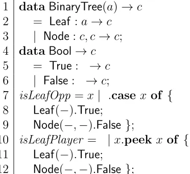
3.9 Examples of using the case and peekconstructs. . . 28

3.10 Type expressions in Compositional Pola. . . 29

3.11 Abstract syntax for type definitions in Compositional Pola. . . 30

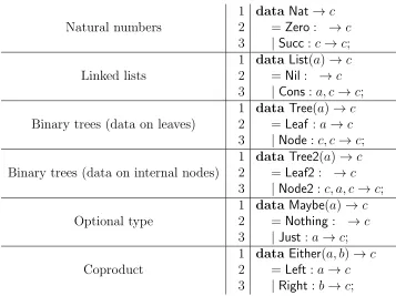
3.12 Example inductive data types in Pola. . . 31

3.13 Example coinductive data types in Pola. . . 31

3.14 Syntax for terms in Compositional Pola. . . 33

3.15 An example of Compositional Pola syntax, defining two functions,addand append, which operate on inductive data. . . 34

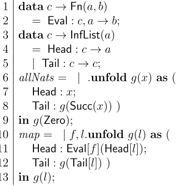
3.16 An example of Compositional Pola syntax, defining two functions,allNats and map, which operate on coinductive data. . . 34

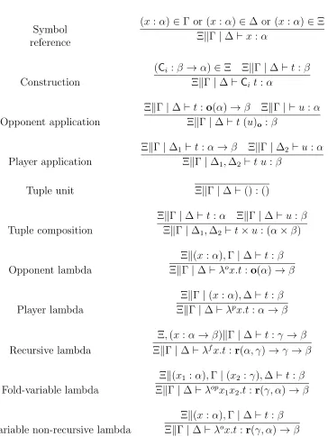
3.17 Typing rules for simple terms. . . 37

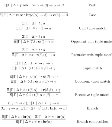
3.18 Typing rules for simple branches and pattern-matching. . . 38

3.19 Typing rules for inductive recursive terms. . . 38

3.20 Theparityfunction, which determines the parity of the natural numberx, and its auxiliary functionnot, both given in both Pola and Compositional Pola syntaxes. . . 39

3.21 A continuation of the derivation below. . . 40

(8)

3.24 A type derivation of the parity function given in figure 3.20. . . 41

3.25 Typing rules for coinductive terms. . . 43

3.26 TheallNatsfunction, which produces the infinite list of all natural numbers. 44 3.27 A continuation of the below derivation. . . 45

3.28 A continuation of the below derivation. . . 45

3.29 A type derivation of the function allNatsgiven in figure 3.26. . . 46

3.30 A hypothetical exponential function which does not rely on duplication of player variables. expXwould compute the value 2x_{for any natural number} x if it were able to be typed. . . 48

3.31 Operational semantics for inductive terms in compositional Pola. . . 49

3.32 Operational semantics for coinductive terms in compositional Pola. . . . 50

3.33 Basic rules of type inference. . . 53

3.34 Rules of type inference for pattern matching. . . 54

3.35 Rules for halting pattern matching. . . 55

3.36 Rules of type inference for tuples. . . 55

3.37 Rules of type inference for fold constructs. . . 56

3.43 Type inference of the parity function given in figure 3.20. . . 61

3.44 Rules of inference for non-recursive coinductive terms. . . 62

3.45 Rules of inference for recursive coinductive terms. . . 63

3.48 Type inference on the allNats function given in figure 3.26. . . 64

5.1 A short compositional Pola function which prefixes its argument, a list of natural numbers, with the number 0. . . 75

5.2 Basic rules of size inference. . . 79

5.3 Rules of size inference for case constructs. . . 81

5.4 Rules of size inference for fold constructs. . . 82

5.5 A continuation of the derivation given in figure 5.6. . . 84

5.11 Size bound inference for the addfunction given in figure 3.3. . . 86

5.12 Rules of size inference for non-recursive coinductive size bounds. . . 87

5.13 Size bound inference on the non-recursive coinductive Pola term ( Eval : x.Succ(x) ). . . 89

(9)

5.14 Rules of size inference for recursive coinductive size bounds. . . 91

5.17 Size inference on the allNats function. . . 93

5.18 A brief summary of each of the 10 definitions introduced in this section. . 97

5.19 Time bounds for simple Compositional Pola terms. . . 104

5.20 Time bounds for inductive constructs in Compositional Pola. . . 105

5.24 Time bound inference for the add function given is figure 3.3. . . 107

5.25 Time bounds for coinductive terms. . . 109

5.26 Potential time bounds for simple Compositional Pola terms. . . 110

5.27 Potential time bounds for inductive constructs in Compositional Pola. . . 111

5.28 A simulation of a Deterministic Turing Machine in Pola. This depends on the functions step, accepting and q to be defined appropriately for the given Turing Machine. . . 115

6.1 An implementation of the less-than-or-equal-to function, leq, in Composi-tional Pola and Pola. . . 117

6.2 A continuation of the derivation given below. . . 118

6.4 Continuation of the derivation given below. . . 119

6.5 Continuation of the derivation given below. . . 119

6.8 Time bound inference for theleq function given in figure 6.1. . . 121

6.9 An implementation of the insert function, insert, in Compositional Pola and Pola. . . 122

6.10 An implementation of the insertion sort function, insertionSort, in Com-positional Pola and Pola. . . 123

6.11 A comparison of type inference rules for the peek construct in Composi-tional Pola (top) and Affine-Free ComposiComposi-tional Pola (bottom). . . 123

6.12 An example of exponential-time behaviour in Affine-Free Compositional Pola. . . 124

6.13 A solution to the Quantified Boolean Formula problem, given in Ex-ploratory Compositional Pola. . . 126

6.14 The simplified typing rules of the peek construct in Compositional Pola (top) and Dangerous Compositional Pola (bottom). The introduction of variables of type α is not given in these rules, for brevity. . . 128

6.15 An example of how to generate an exponential-time function if safe and dangerous type restrictions are not put on records. . . 129

6.16 Modified typing rules for records in Dangerous Compositional Pola. . . . 129

6.17 A second example of an exponential-time function if safe and dangerous type restrictions are not properly put on records. . . 129

(10)

5.1 The three forms of sequents used during time bound inference. . . 103

(11)

Chapter 1 Introduction

Nearly every programming language in common use today—for instance, C, Java, Lisp, PHP, Perl, Javascript, Matlab—is universally powerful. That is, anything which can be computed can be computed using these languages1_{. This is a benefit in allowing an}

expressive and natural style of programming, and in allowing computationally intensive functions, such as exponential-time functions, to be written, but it is an impediment to static analysis. It is a clear consequence of the Church-Turing thesis that one cannot provide a method which, in general, will determine the running time of a function. This thesis will explore inferring running times, but will focus on a computational model which is not universally powerful and hence to which the Church-Turing thesis is not applicable. This thesis describes the programming language Pola, a programming language which is not universally powerful. Specifically, it is limited to the polynomial-time functions: it is impossible in Pola to write a function which does not halt in time polynomial with respect to the size of its input. We will then show how this restriction placed on Pola allows the practical bounds of running times of functions written in the language to be automatically inferred by a Pola interpreter or compiler.

The primary applications of a language like Pola can most clearly be seen in hard real-time software systems, such as medical devices, automotive controls or industrial controllers. These systems consider any software component which does not meet its specified time constraints to be a system failure. Having an automated guaranteed bound on running time from a compiler would relieve the burden from the programmer and would be more reliable than testing to ensure the software meets its specifications. Since Pola is not universally powerful, it would likely never comprise the totality of a software system, but could provide the primary CPU-bound components in conjunction with other software components.

1.1 Functional languages

Pola is a functional programming language. The two hallmarks of functional program-ming are: firstly, that functional programs are declarative, in that functions consist of expressions to evaluate, rather than featuring a sequence of statements or instructions 1_{This ignores the technicality that on a physical computer one is bound by a fixed amount of memory.}

(12)

1 public static int sumArray(int[ ]xs) {

2 int sum = 0;

3 for (int i= 0;i <xs.length;i++) 4 sum+ =xs[i];

5 return sum; 6 }

Figure 1.1: A Java method which sums the elements of an array of integers and returns that sum.

1 sumArray [ ] = 0

2 sumArray (x:xs) =x+sumArray xs

Figure 1.2: A Haskell function which sums the elements of a list of integers and returns that sum.

to execute, as in an imperative language; and secondly, that functional programs do not allow for side-effects such as global variables or direct access to memory locations. The second hallmark mentioned allows what is sometimes calledreferential transparency, wherein a term or subterm may be considered in isolation since its behaviour is guaran-teed to be the same regardless of the state of the rest of the program.

To demonstrate by way of example, consider the Java method given in figure 1.1 which sums the elements of an array of integers. Note its use of a for loop and the use of assignment statements, on lines 2 and 4, which change the value of a variable. In contrast, consider the Haskell function given in figure 1.2, which does not use statements or destructive updates, but rather relies on recursion and pattern-matching. On line 1 we match the case that the input list is empty. On line 2 we match the case that the input list is not empty, but rather has a head x (an integer) and a tail xs (a list of integers), with the resulting value being declared as an arithmetic expression involving those two. Finally, consider figure 1.3 which is the same function written in Pola. It is more verbose than that of the Haskell function and requires the “on-the-fly” introduction of a recursive function, f, to accomplish the task, but is structurally similar to that of the Haskell function. Line 2 matches the case where the list is empty (the Nil case) and line 3 matches the case where it is not empty (the Conscase), where it has a headz and a tail zs.

Practical general-purpose functional languages, such as Lisp, Haskell or Concurrent

1 sumArray =x| .fold f(y) as {

2 Nil.0;

3 Cons(z,− |zs).add(z, f(zs)) }

4 in f(x);

(13)

1.2. Implementation 3

Clean, find some way to allow I/O—which is a side-effect—to be integrated into the functional framework of the language. This is currently absent in Pola, primarily as it would needlessly complicate the language and distract from the main focus of this thesis.

1.2 Implementation

An implementation of the Pola language can be downloaded and examined, available un-der a free software licence. The implementation is an interpreter written in the Haskell programming language. It performs parsing and type inference according to the specifi-cations for the Pola language given in chapter 3 and evaluates expressions according to the operational semantics of chapter 3. Note that, in chapter 3, two different notations are given for the language: Compositional Pola, which is useful for exposing the rules of inference for the language with great precision; and Pola, which is the language the implementation targets, and is more useful for programming use.

The implementation also offers automated size and bounds inference, as discussed in chapter 5.

The Dangerous Pola variant of Pola discussed in section 6.3.3 is implemented, as it offers a greater level of expressiveness to the programmer than Pola. However, none of the other variants discussed in chapter 6 are supported by the implementation.

To aid the reader in navigating the source code, Pola’s implementation has been written in a literate style, a style of programming developed by Donald Knuth to aid in programmer comprehension [24].

The reader is invited to explore the source code for the reference implementation of Pola at the following website and git code repository:

https://gitlab.com/professormike/pola

1.3 Summary

(14)

(15)

Chapter 2 Literature survey

Static analysis is the process of inferring, from a description of a computation, significant properties of that computation. The proof of the undecidability of the halting problem— i.e., the problem of giving an algorithm to universally decide if a Turing machine halts or not—provides an early upper bound on the capabilities of static analysis. An algorithm to determine how long any C program takes to run, for example, is clearly impossible, as the halting problem can be reduced to it.

Even if determining a running time were possible, it may not be useful. A static analysis which takes as long to compute as the computation under analysis is not of great use.

In spite of these barriers, there is a pressing need for static analysis. Software pub-lishers might like to know how long a computation will take, or how much memory it will require, or, conversely, what the minimum hardware specifications are for some task. In embedded systems, for example, or systems with real-time requirements, it is imperative that it can be guaranteed with certainty that software will not exceed pre-determined requirements.

This chapter will deal with previous work in statically determining the consumption of resources, namely time and memory usage. These two resources are not the only resources that a piece of software might require, but they are the most general, and in any case the techniques used to determine them can be modified to determine other resource requirements.

2.1 Abstract interpretation

Abstract interpretation involves interpreting a language, usually a universally powerful language, in an “abstract” manner. For instance, consider the following C program:

static int foo(int x) { return x * 2;

}

int main(void) { int a = foo(3);

(16)

int b = foo(4); return a + b; }

We begin interpreting (or executing) the program frommain as usual. One way to carry out abstract interpretation is to have a global binding forfoo’sxvariable, not dependent on any context. During the first function call to foo, x has a value of 3 and we assign a value of 6 to a. During the second function call to foo, x has a value of 3,4 (either 3 or 4, since we can’t distinguishx based on where it’s called from) andb gets a value of 6,8. We say, abstractly, that the program returns a value of 12,14.

Different abstract interpreters offer different abstract semantics. In abstract inter-pretation we “interpret” the program according to the usual program flow, i.e., for a C program we start “interpreting” at the first statement and move towards the last state-ment. Also, for any construct which offers the possibility of undecidability, we “abstract” the semantics to deal with sets of values instead of concrete values.

Gustafsson et al. provide a simple abstract semantics for C as described above, as a means of determining flow analysis [15]. The information from the flow analysis, deter-mining the value ranges of variables before and after loops, is then used to help determine worst-case execution time.

The idea of abstract interpretation came from Cousot and Cousot [8] and had very strict semantics for a program represented as a lattice. It encompassed data flow analysis, in that all data flow analysis could be written as abstract interpretation [8]. This model has limited utility with functional languages due to the referential transparency provided by those languages.

2.2 Restricted models of computation

The implications of the undecidability of the halting problem are that, to determine the running time of a computation more generally, one must abandon the hope of certainty, or one must abandon the hope of universality. The latter is promising because much of the software written today is, in the grand scheme of computability theory, not very complex: many software problems would be in the class of polynomial time or maybe even more restricted complexity classes such as those in logarithmic space. Many of the algorithms in use today halt in a time polynomial with respect to their input, and so for many uses it will suffice to have a static analysis which only works on that class of algorithms.

Strategies for restricting computational power, while still allowing useful programs to be written, include limiting the growth of the functions, limiting the structure of the programs and the primitives provided and using types.

2.2.1 Primitive recursion

(17)

2.2. Restricted models of computation 7

1. f(x) = 0 (zero);

2. f(x) = x+ 1 (successor);

3. f(x1, . . . , xn) = xi for some i, n ∈Nsuch that i≤n (projection);

4. f(x1, . . . , xn) = h(g1(x1, . . . , xn),· · · , gm(x1, . . . , xn)) for some m, n ∈ N where h

and each gi are primitive recursive (composition); or

5. f(0, x1, . . . , xn) =g(x1, . . . , xn) and

f(y+ 1, x1, . . . , xn) = h(x1, . . . , xn, y, f(y, x1, . . . , xn)) for some n ∈N where g and

h are primitive recursive functions (primitive recursion).

This general model of primitive recursion, of recursing over the structure of a datum (in this case, the structure of a natural number expressed in Peano arithmetic), will become a strong part of Pola, as seen in section 3.1.2.

Limited recursion and the Grzegorczyk hierarchy

A limited recursive function is a primitive recursive function, as described above, with the restriction that its value must be bounded by some base function, i.e., one that is not built up through recursion. We take the definition of primitive recursion above and modify clause 5. Consequently, the clauses for defining a function f are as follows:

1. f(x) = 0 (zero);

and each gi are primitive recursive (composition); or

5. f(0, x1, . . . , xn) =g(x1, . . . , xn) and

h are primitive recursive functions and also f(y, x1, . . . , xn) ≤ j(y, x1, . . . , xn) for

ally, x1, . . . , xn wherej is some function previously defined by rules 1 to 4 (limited

recursion).

The definition of limited recursion has great influence in the definition of the Grzegorczyk hierarchy, and has the unfortunate side-effect that it becomes undecidable whether or not some function is limited recursive.

The Grzegorczyk hierarchy [31] is a hierarchy of sets of functions. We first define a set of functions, Ei, for all i ∈ N. E0, the first function, has two parameters, x, y ∈ N.

All other Ei functions have a single parameter. TheEi functions are defined as follows:

E0(x, y) = x+y (2.1)

E1(x) = x2+ 2 (2.2)

(18)

From these functions we can define the hierarchy of sets of functions, denoted Ei _for

some natural numberi. The first set in the hierarchy,E0_{, is equal to the zero functions, the}

successor functions, the projection functions, the composition functions (over functions inE0_{), and the limited recursive functions over functions in} _E0_{. Of note, no} _E

i functions

are in E0_{. Stated precisely, a function,} _f_{, is in} _E0 _{if and only if:}

1. f(x) = 0 (zero);

3. f(x1, . . . , xm) =xi for some i, n∈N such that i≤n (projection);

4. f(x1, . . . , xm) = h(g1(x1, . . . , xm),· · · , gp(x1, . . . , xm)) for some m, p ∈ N where h

and each gi are in E0 (composition); or

5. f(0, x1, . . . , xm) = g(x1, . . . , xm) and

f(y+ 1, x1, . . . , xm) =h(x1, . . . , xm, y, f(y, x1, . . . , xm)) for somen ∈Nwhereg and

h are in E0 _{and also} _f₍_{y, x}

1, . . . , xm) ≤ j(y, x1, . . . , xm) for all y, x1, . . . , xm where

j is in E0 _{(limited recursion).}

For each n > 0, we define En _{as the basic functions (zero, successor, projection),}

composition functions (over functions in En_{), limited recursive functions (ibid), as well}

as the functionsE0 andEn. Stated precisely, a function,f, is inEnfor somen∈N, n >0

if and only if:

1. f(x) = 0 (zero);

and each gi are in En (composition); or

5. f(0, x1, . . . , xn) =g(x1, . . . , xn) and

h are in En _{and also} _f₍_{y, x}

1, . . . , xn)≤j(y, x1, . . . , xn) for all y, x1, . . . , xn where j

is in En _{(limited recursion); or}

6. f =Ek fork < n.

Note that E1 _{includes all functions in which the result is a constant number of}

addi-tions of its parameters,E2 _{includes all functions in which the result is a constant number}

of multiplications or additions of its parameters, E3 _{includes all functions in which the}

(19)

Predicting time complexity of recursive functions

Restricted models of computation can prove useful for predicting time complexity of functions. The Grzegorczyk hierarchy itself comprises the exponential hierarchy [2], though there is the possibility to provide more precise predictions.

R.W. Ritchie [30] was one of the first to formalize predicting resource requirements for functions in a primitive recursive scheme. He created a hierarchy F1, F2, F3, . . . between

E2 _and _E3_{. Where} _F

0 =E2, a function f ∈ F1 if ∃g ∈ F0 such that, if Tf(x) is the time

required to compute f, then Tf(x) ≤g(x). Similarly, for all i∈ N, f ∈ Fi+1 if ∃g ∈ Fi

such that Tf(x)≤g(x) for allx.

Perhaps more interesting, however, was Ritchie’s formalizing of a method to express the running time of primitive recursive functions, using a very abstract computational model for determining “time.” For the base functions, the definitions of Tf are more

obvious. For composition and primitive recursion, though, they are less obvious. He showed that:

• iff(x, y) =h(x, g(y)), thenTf(x, y) =|x|+|y|+ max{|x|+Tg(y), Th(x, g(y))}; and

• if f(0, x) = g(x);f(y + 1, x) = h(x, y, f(y, x)), then Tf(y, x) = 2(|x| + |y| +

max{maxz≤y{Th(x, z, f(z, x))}, Tg(x)}.

Limitations to primitive recursion

Lo¨ıc Colson showed some practical concerns with using primitive recursion as a basis for programming languages [7]. The function:

min(a, b) =

a , if a < b b , otherwise

can be implemented quite easily in a primitive recursive framework. However, there does not exist a primitive recursion algorithm which will compute it in O(min(a, b)) time. While this specific instance can be resolved easily in a practical programming language, for example by the introduction of a constant-time less-than (‘<’) operator, it neglects the wider problem presented, namely that in a primitive recursive scheme, one cannot efficiently recurse through two data simultaneously. Any function which needs to do something of the sort has a greater time complexity in primitive recursive frameworks than in unrestricted computational frameworks [7].

2.2.2 Hofmann survey

Martin Hofmann presents an excellent survey of programming languages capturing com-plexity classes [21]. A programming language is said to capture a comcom-plexity class C if every well-defined program in that language has time complexity in C. Of especial note is that in the introduction to this survey, Hofmann specifically brings up the example of guaranteeing resource restrictions in embedded systems.

(20)

recursed on the length of x (when written as a string), not on the value ofx. Successor functions were notation-wise, so if the number were represented in binary, there would be two successor functions, S0(x) = 2x and S1(x) = 2x+ 1, effectively adding a ‘0’ or

‘1,’ respectively, to the end of x. Cobham showed that these successor functions, zero functions, composition functions, projection functions, limited recursion by notation, and the smash function, x#y = 2|x|·|y|, equal the polynomial-time functions.

The same paper also showed that all functions inE2_{, the third set in the Grzegorczyk}

hierarchy, require at most linear space.

Gurevich showed that primitive recursion over a finite domain, i.e., where the succes-sor function has an upper limit, is exactly the class of programs operating in logarithmic space [14].

The two previous models can be regarded as being somewhat awkward or artificially restricted, Cobham’s method especially because it is undecidable whether a program is well-formed or not. Bellantoni and Cook provide a model based on primitive recursion more naturally bounded to polynomial-time functions [1]. Function parameters are di-vided into “normal” and “safe” parameters, denoted asf(x;y), where parameters before the semi-colon (x) are “normal” and parameters after the semi-colon (y) are “safe.” Nor-mal parameters may recursed over, but safe parameters may only be used in composition. Further, the result of a recursive function may only be used in composition.

While Pola does not directly use the idea of “normal” and “safe” parameters, it does borrow the notion of having two classes of variables which have differing restrictions on them, as will be seen in section 3.1.2.

Loop programs

One model of computation proposed in the late 1960s is that of loop programs, which is equivalent in power to the class of the primitive recursive functions [26]. A loop program operates over an aribtrary, but finite, number of named registers (canonically X and Y

and so on). Each register holds a natural number of unbounded size. A loop program is a finite sequence of instructions, where each instruction is one of:

1. X =Y for two registers X and Y; 2. X =X+ 1 for some register X; 3. X = 0 for some registerX; 4. LOOP X for some register X; or 5. END.

There is a further restriction upon the structure of loop programs, which is thatLOOPX

and END instructions must be paired.

(21)

instructions are “paired,” the instructions I1, . . . , In will be executed serially X times.

For instance, if X has the value 3 when such a block is encountered, the instructions

I1, . . . , In, I1, . . . , In, I1. . . , Inwill be executed. The variable which is used to control the

loop (X, in this case) must be invariant.

2.2.3 The Hume languages

Hume, the Higher-order Unified Meta-Environment, is a hierarchy of programming lan-guages aimed at writing correct and verifiable code for embedded systems. The simplest layer of Hume, HW-Hume, disallows recursion entirely, allowing only constant transfor-mations between input bits and output bits. FSM-Hume allows non-recursive first-order functions and non-recursive data types. Template-Hume allows pre-defined higher-order functions (such as map oriter, found in typical functional languages), user-defined first-order functions, and inductive data types. PR-Hume allows primitive recursive functions over inductive data types. Finally, Full Hume is an unrestricted, Turing-complete lan-guage [17].

Michaelson early on develops a method for bounding recursion in a simple lambda-calculus–based language, either by eliminating recursion entirely or by allowing a primi-tive recursion [27].

Hardware level

The lowest level of Hume is HW-Hume (hardware Hume), which provides simple pattern bindings [16]. For instance, a parity checker can be written as follows:

box parity

in (b1 :: Bit, b2 :: Bit) out (p :: Bit)

match

(0, 0) -> 0 | (0, 1) -> 1 | (1, 0) -> 1 | (1, 1) -> 0

No recursion or iteration is offered [16], which limits its computational utility.

Finite state machine

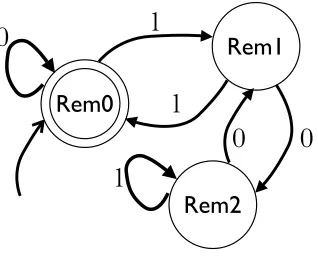
The finite state machine level of Hume, FSM-Hume, provides a syntax for describing the behaviour of generalized finite state machines (abstracted to inductive data types in general, not just symbols) in the expression syntax of Hume [18]. Figure 2.2.3 contains a finite state machine for determining if a binary number is divisible by 3.

In FSM-Hume, this would be written as:

data State = Rem0 | Rem1 | Rem2; type Bit = Word 1;

(22)

Rem1

Rem2 Rem0

0

1

0

1

Figure 2.1: A finite state machine to decide if a binary number is divisible by 3.

in (s :: State, inp :: Bit) out (s’ :: State, out :: Bool) match

The remainder of the program must happen at one level lower, in HW-Hume, to wire the new “box.”

stream input from "std_in"; stream output to "std_out"; wire input to div3.inp;

wire div3.s’ to div3.s initially Rem0; wire div3.out to output;

Templates

Applying a finite transducer to input, as in FSM-Hume, works for simple examples, but becomes tedious when trying to apply the same transformation to each bit in a vector, for instance. Template-Hume offers some pre-defined higher-order functions to achieve this end [18].

For instance, to square each number in a vector:

square :: Int -> Int; square x = x * x;

squareVector :: vector m of Int -> vector m of Int; squareVector v = mapvec square v;

(23)

Primitive recursion

PR-Hume is a typical functional programming language, permitting recursion, but bound-ing the recursion to the class of primitive recursive functions [18]. Since determinbound-ing if an arbitrary function is primitive recursive is undecidable and PR-Hume offers no structural restrictions to bound the recursion, PR-Hume relies on partial analysis to determine if a function is primitive recursive [18].

The mechanism for turning unrestricted expressions into forms that guarantee primi-tive recursion relies on single-step reductions and looking for syntactic expressions of the form:

pr y x = f y x (pr (h y) (g x))

whereyis the variable which must strictly decrease in size,his a “size-reducing” function and f and g are functions already analysed to be primitive recursive [27].

2.2.4 Categorical approaches

Category theory has offered a few approaches to creating restricted programming lan-guages, often called categorical computing. Common among categorical approaches is the use of inductive and coinductive datatypes.

For instance, stateless attribute grammars used in parsing can be written as catamor-phisms [12]. The grammars are written as inductive data types, with each alternative in a grammar rule corresponding to a constructor in an inductive datatype. Parsing then is taken as a catamorphism over this datatype [12].

Paramorphisms

One method of bounding recursion is to disallow explicit recursion entirely and allow primitives for performing recursion. As Dijkstra famously warned of the perils of goto statements [11], Meijer et al. warn of the perils of unrestricted recursion [25]. They provide a proposal to build more structured programs, based on category theory and unrestricted inductive data types, using various primitives for recursion.

Catamorphisms are a class of functions which replace the constructors of an induc-tively defined data structure, effecinduc-tively recursing through each node in the structure. For instance, consider the inductive definition of a binary tree:

T(α) := Leaf |Node(α, T(α), T(α))

A catamorphism to sum the nodes of a tree could, in a typical language allowing recursion, be written as:

c(v) =

0 , if v =Leaf

va+c(v1) +c(v2) , if v =Node(va, v1, v2)

For brevity and clarity, the authors suggest the use of “banana brackets” to write cata-morphisms, so that the above function would be written as:

(24)

Note that the expression describing the Leaf component of the banana bracket is nullary (i.e., is abstracted over no parameters) whereas the expression describing the Node component of the banana bracket is ternary, corresponding to the fact that the Node constructor has 3 subterms.

Anamorphisms are a class of functions which allow one to construct a member of an inductive type from a seed value. In the context of a function g : α → (β, α, α) and a predicate functionp:α→Bool, an example anamorphism might be written in a typical functional language as:

f(v) =

Leaf , if p(v)

Node(a, l, r) , otherwise, where (a, l, r) =g(v)

One thing to note is that even though anamorphisms often produce data structures of infinite size, in a lazy language, a catamorphism which acts on an anamorphism will always halt. Secondly, unlike with catamorphisms, anamorphisms are almost always given in the context of a function, in this case g.

The authors use “concave lenses” to denote anamorphisms, and the above example would be written as:

a = [(g, p)]

A sort of combination of the two, holomorphisms are recursive functions in which the call tree is isomorphic to an inductive data structure. For instance:

h(v) =

c , if p(v)

va+h(v1) +h(v2) , otherwise, where(va, v1, v2) =g(v)

This is written using “envelope” notation, and the authors write it as:

h= [[(c, λa.λl.λr.a+l+r),(g, p)]] They also show that for any data type and for any a, b, c, d:

[[(a, b),(c, d)]] = (|a, b|)◦[(c, d)]

Meijer et al.’s paper was the first to formally introduce paramorphisms to a program-ming language. A paramorphism is exactly like a catamorphism but the constituent functions accept extra arguments for attributes which have not undergone recursion. For instance, consider the factorial function over the unary natural numbers:

f(n) =

1 , if n =Zero

(1 +p)·f(p) , if n =Succ(p)

Note that the attribute p is used both on its own and as an argument to the recursion. Being able to use p on its own is what distinguishes this from a catamorphism. The authors propose “barbed wire” notation for writing paramorphisms, and this would be written as:

f ={1, λpp.ˆ(1 + ˆp)·p}

These paramorphisms strongly relate to the fold constructs in Pola, as introduced in section 3.1.2.

(25)

Charity

Charity is the most successful categorical programming language. It is centred around inductive and coinductive datatypes, with computations performed using catamorphisms (“folds”) and anamorphisms (“unfolds”) [5, 13]. It is not universally powerful—every program must halt given finite user input—but it is strictly more powerful than primitive recursion.

More properly stated, Charity offers three combinators (and their duals): the “fold” or catamorphism (“unfold” or anamorphism), map (also a “map” in the dual), and case (record). Maps and cases (records) are special cases of catamorphisms (anamorphisms), however.

A Master’s student of Cockett’s extended the language to Higher-order Charity [34]. Inductive types were left unchanged, but coinductive types could have their destructors parameterized over some higher-order function, which led to efficient min and zip func-tions. Further, Higher-order Charity offered an object-oriented system, built on top of higher-order coinductive types, where an unapplied anamorphism was a class, an applied anamorphism was an instance, and a parameterized destructor was a method.

Cockett describes the workings of the standard Charity interpreter, describing the basic datatypes (natural numbers, lists, trees) and co-datatypes (co-natural numbers, co-lists, co-trees). He also explains how to use common programming idioms in Charity such as “dualing” (converting between a datatype and its cognate co-datatype) and dynamic programming in Charity [5].

As a proof that Charity is more powerful than primitive recursion, a program to calculate Ackermann’s function is provided [6]. Ackermann’s function is defined as:

ack(0, n) = n+ 1 (2.4)

ack(m+ 1,0) = ack(m,1) (2.5)

ack(m+ 1, n+ 1) = ack(m,ack(m+ 1, n)) (2.6) One can consider an infinite table, where the value at column m and rownis ack(m, n). Equation 2.4 says that each entry has valuen+ 1 in column 0 for row n:

0 · · ·

0 1 · · ·

1 2 . . .

..

. ... . ..

In other words, column 0 is tail(nats) wherenats is the infinite list of natural numbers. Equation 2.5 says that each entry in row 0 has the same value as in row 1 of the previous column:

0 1 · · ·

0 1 2 · · ·

1 2 · · ·

2 3 · · ·

..

(26)

Finally, equation 2.6 says that for some other row and column m+ 1 and n+ 1, we look in the table at co-ordinates (m+ 1, n) to find value i, then look again in the table at co-ordinates (m, i) to find the new value at (m+ 1, n+ 1). Since all values needed have been previously defined, this is a dynamic programming problem, and we end up with the correct infinite table of:

0 1 2 3 · · ·

0 1 2 3 5 · · ·

1 2 3 5 13 · · ·

2 3 4 7 29 · · ·

..

. ... ... ... ... . ..

Cockett’s Ackerman construction creates a Charity function, col m, which takes as its argument the infinite coinductive list of the previous column. It uses an unfold to destruct that list into a new infinite coinductive list. With the use of another function to retrieve an element from the infinite list at a particular index, it follows that we can compute

ack(m, n) for any given natural numbersmand n, thus making Charity able to compute functions beyond primitive recursive, while still remaining recursive.

Like Charity, Pola does have possibly-infinite coinductive structures much like Charity does, as will be seen in section 3.1.3, but will have typing restrictions to ensure that nothing super-polynomial can be produced through them.

2.3 Type theoretic approaches to determining

re-source consumption

A popular area of research in attempting to track memory usage, or resource consumption in general, is type theory. For instance, Herding’s Master’s thesis describes how to augment functions in the specification language CASL to track memory state [19]. The general idea is to encode resource consumption information into the type of a symbol (e.g., a variable or function). This allows composing components of a larger program together using type matching or type inference to gain information on the resource consumption of the program as a whole. We will see in chapter 5 that considering resource consumption to be a part of a symbol’s type information will become useful for Pola.

2.3.1 Stack language

Saabas and Uustalu offer a type-theoretic approach to stack-based programs [33, 32], interesting because it deals specifically with programs with jumps (“gotos”) without any explicit structure. The major motivation is to provide techniques for generating proof-carrying code for low-level programs.

The first paper dealt with simple unstructured code with gotos [33]. The second paper extended the language to allow operand stack operations [32].

The Push language described in [33] defines “a piece of code” (program) to be a

(27)

2.3. Type theoretic approaches to determining resource consumption17

instruction. Instr, the set of instructions, is defined as the instructions load, store,push, goto (unconditional jump), gotoF (conditional upon the top operand, read as “goto if false”), plus some simple stack-based logical and arithmetic operations (add, eq, and so on). There is also a finite set of registers used by the load, store and push instructions. All of load, store and push have a single register operand; goto and gotoF have natural-number constants as their sole operands;add,eq and so on take their operands from the stack and do not deal with registers at all.

The authors structure the Push code into a finite union of non-overlapping labelled

instructions, creating a new language called SPush, where an SPush program is a

binary tree of labelled instructions, i.e., a binary tree where each leaf is a (_N,Instr) pair. Construction is associative. The semantics are identical betweenPush and SPush, but

using SPush allows the definition of a Hoare logic through composition. The authors

construct a sound and complete Hoare logic.

Finally, the authors weaken the Hoare logic into a typing system. The type system ensures safe stack usage [33]. Any operations beyond stack usage are not considered.

2.3.2 Memory bounds

Hofmann and Jost provide a method for finding linear bounds on memory allocation in a first-order functional language, called LF, but in the context of explicit memory deallocation and in the presence of a garbage collector [22]. The authors excuse the restriction to first-order functions foremost because it is fruitful to do so, but also because one can work around it through code duplication. They introduce types with simple first-order functions in which data must be units (the data type with only one datum in its domain, often written as 1 or () in functional languages), Booleans, lists, Cartesian products, or unions:

A := 1|B|L(A)|A⊗A|A+A (2.7)

F := (A, . . . , A)→A (2.8)

where A is a zero-order type and F is a first-order type. The function SIZE(−), which returns the natural number indicating the number of memory cells needed to store a datum of that type, is defined on all zero-order types.

A defining characteristic of the LF language presented is that it has two methods for pattern-matching: the match construct (destructive pattern matching) and the match’ construct (non-destructive pattern matching) [22]. In the former, the datum being matched is deallocated from memory, while in the latter, the datum being matched can be referenced in subsequent parts of the program.

For the purposes of determining memory usage, the authors define a new language, LF_♦, in which the data types are augmented with size annotations, where _Q+ _{is the set}

of positive rational numbers:

A := 1|B|A⊗A |R+R|L(R) (2.9)

R := (A, k) for somek ∈_Q+ _(2.10)

(28)

TheRtypes are read as “rich types” because they carry information about their memory requirements. Note that functions accept parameters of “plain” (A) types, but return a rich value. They set up type judgements to determine resource requirements. For instance, the simple rule which types the expression () to be of the unit type:

n≥n0

Γ, n `Σ () : 1, n0

is read as “in the context Σ under environment Γ with n free memory cells, () is of type 1 with n0 or more unused memory cells left over.” More interesting cases are to see how memory requirements change when doing a destructive pattern match on a list (equation 2.12) as compared to a non-destructive pattern match on a list (equation 2.13):

Γ, n`Σ e1 :C, n0 Γ, xh :A, xt:L(A, k), n+ SIZE(A⊗L(A, k)) +k `Σ e2 :C, n0

Γ, x:L(A, k), n`Σ matchxwith(nil ⇒e1;cons(xh, xt)⇒e2) :C, n0 (2.12)

Γ, n `Σ e1 :C, n0 Γ, xh :A, xt :L(A, k), n+k`Σ e2 :C, n0

Γ, x:L(A, k), n`Σ matchxwith(nil ⇒e1;cons(xh, xt)⇒e2) :C, n0 (2.13)

Finally, the authors devise a system for inferring annotations in the program, such that the programmer does not necessarily need to explicitly annotate sizes for each function or datum.

Hofmann and Jost also introduce an amortized system of determining memory bounds [23]. They propose a Java-like language where each value carries with it some “potential” and each operation carries with it some amortized costs. The sum of the amortized costs plus the potential of the input to an operation then provides a bound.

Each class is augmented into a “refined class,” which is a class that has some potentials attached, through what are called views. For instance, in the view a, the Cons class carries a potential of 1 (indicating that operations on it have an extra cost of 1, stripping off the potential associated with the Cons) whereas in another view b, the same Cons

class carries a potential of 0. Note that a single object in the Java-like language can be, and often is, considered from different views with different potentials and thus can be of different types.

A view carries three pieces of information: the potential of the class itself, the potential of each attribute (where each attribute has both a “get-view,” the potential of reading the attribute, and a “set-view,” the potential of writing to the attribute) and the potentials for each of its methods, which are functions of its arguments.

For instance, consider a program to append two lists:

abstract class List { abstract List append(List x); }; class Nil { List append(List x) { return x; } };

class Cons { int head; List tail;

(29)

2.4. Static memory management 19

r.head = this.head;

r.tail = this.tail.append(x); return r;

} };

We introduce two views: a and b. In the view a, Cons has potential 1 and all other classes have potential 0; in the view b, all classes have potential 0. The method append is well-defined only asLista×Listb →Listb, i.e., it is only defined as operating on lists in the view a, taking arguments in the viewb and returning values in the viewb.

To prove (correctly) that summing a list consumes memory proportional to its first operand, but irrespective of its second operand, we need to prove judgements such as:

this :Nila, x:Listb `0₀ (return x) :Listb (2.14)

this :Consa, x:Listb `₀1 (Listr= new...) :Listb (2.15) Here the notation `m

m0 carries the semantics that the amount of free heap space must be

at least m plus the potential of the expression given on the right-hand side, and that the m plus the potential of the result is at most the amount of free heap space after execution. In this case, since the operand is in the a view, it carries the cost of the execution in terms of its potential (e.g., since the potential of Consis 1, a list of length 5 will have 5Conses and thus have a potential of 5) and the cost of the append function will be 1 for each potential of the input.

The authors prove soundness of the typing system. One nice feature of the system is that it is not weak with respect to divide-and-conquer methods as similar systems are. For instance, when writing Quicksort in the na¨ıve way (choosing the first element of a list as the pivot), one often has to judge that, after splitting up the remainder of the list, both lists have maximum size n −1, where n is the length of the list. When merging the two lists back together, one finds a bound on the size of the list as 2n −1, rather than the proper n. This can erroneously lead one to believe that Quicksort consumes exponential space. In this system, one requires explicit judgements for contraction, so that when aliasing objects, the potential is divided among them [23].

The major downside of the Hofmann and Jost system is that memory bound inference is not considered and neither is any type inference system.

2.4 Static memory management

(30)

Region-based memory management is a memory management model added to the ML language [36]. It annotates ML types and ML expressions with region variables where a region variable refers to a statically allocated and deallocated region of memory. Unlike in a simple stack-based memory management system, we have a finite stack of not just finite memory cells, but a finite stack of unbounded regions of memory which can grow dynamically. Like a simple stack-based memory management system, the regions are lexically scoped and deallocated in constant time.

The major changes to the language are the at expression and the letregion expres-sion. The letregion expression creates a new region, and introduces a corresponding region variable, which exists only within the lexical scoping of theletregionexpression. The at expression is used for atomic constructions indicating which region to allocate it in. As an example:

(λ x.letregion ρin λy.(y,Nil@ρ)atρend x) 10

This function creates a region, ρ, and allocates an object, Nil, in that region. Once the expression is evaluated, ρ is deallocated (and the Nilis destroyed with it).

A fully annotated region-based expression becomes quite unwieldy and there has been work done to automatically infer which regions to place objects in [35].

2.5 Conclusion

There has been work done in the past to study both static analysis techniques on existing programming languages and in developing more explicitly or rigidly structured programs to aid in resource analysis. Developing a flexible programming model that lends itself to automatic inference of resource requirements is still something missing in today’s programming languages, however.

(31)

Chapter 3 Compositional Pola

Twe expositions of a functional language constrained to polynomial-time functions are presented here, Pola and Compositional Pola. Both languages are equivalent in their typing and semantics. Pola is the variant which has been implemented (see chapter 4) and would be used by programmers. However, the language constructs contained within it would be far more complicated to describe and so, in the interest of clarity, a composi-tional form of the language called Composicomposi-tional Pola is described in this chapter, which simplifies and clarifies exposition, definitions and proofs of the language. For most of the chapter, and for all of the introductory examples, we will present examples using the syntaxes of both Pola and Compositional Pola. Pola can be thought of as a “sugared” Compositional Pola, a syntax which makes the constructs more readable. Proofs and detailed descriptions will be based off of Compositional Pola only, however.

3.1 Introductory examples

3.1.1 Recursion-free examples

Figure 3.1 shows simple Pola code that does not use any recursion or complicated data types. It attempts to define two different functions, one called f and the other called g. Both functions aim to have a single parameter, called x, and return a tuple that contains the value of x in both positions of the tuple. The syntax for defining functions in Pola is to begin with the name of the function, followed by an equal sign, following by a list of parameters segregated such that opponent parameters are on the left of a vertical bar and player parameters on the right, followed by a dot, followed by a term.

The example demonstrates one crucial part of Pola which permeates the language: two different types of variables. The function f in figure 3.1 declares the parameter x

1 f =x| .(x, x); 2 g = |x.(x, x);

Figure 3.1: A demonstration of the distinction between opponent and player variables. The function f is legal in Pola, but the function g is illegal.

(32)

1 dataNat→c

2 = Zero:→c

3 | Succ:c→c; 4 dataList(a)→c

5 = Nil:→c

6 | Cons:a, c→c;

7 add =x|y.foldf(a, b) as {

8 Zero.b;

9 Succ(− |n).f(n,Succ(b))}

10 in f(x, y);

11 append =l|m.fold f(a, z)as {

12 Nil.z;

13 Cons(x1,− |x2).Cons(x1, f(x2, z))}

14 in f(l, m);

Figure 3.2: An example of inductive data types and folds in Pola.

before the vertical bar, making it an opponent variable. An opponent variable has no restrictions on where it can be used or how often it can be used. Functionf is therefore a legal function.

The functiong, in contrast, declares its parameterxafter the vertical bar, designating it as aplayervariable. Player variables have an important restriction on their use, namely that they cannot be repeated multiple times in the same term. This will later prove to be an invaluable tool in restricting the computational power of the language. Because the function g attempts to use the parameter x twice, the function g is illegal in Pola.

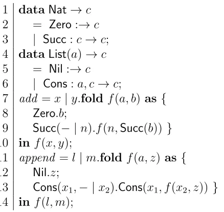
3.1.2 Inductive data types and folds

(33)

3.1. Introductory examples 23

of type Nat. Succ : c → c can be read as defining a constructor, Succ, which takes one parameter of typeNat and produces a value of type Nat.

From these two constructors one can define the natural numbers. From this point forward we will, for clarity, denote natural numbers constructed from these expressions as Arabic numerals with an overhead bar. For instance, the expression Succ(Succ(Zero)) will be denoted as ¯2.

Lines 4–6 define the inductive type of lists. The expression Nil is of type List(a) for all types a. The expression Cons(h, t) is of type List(a) for all expressions h of type a

and expressions t of type List(a). For example, the expression Cons(Zero,Nil) is of type List(Nat). a in this context is a type variable—not itself a concrete type—and List(a) is a parameterized type.

From this point forward we will, for clarity, denote lists constructed from these ex-pressions within square brackets. For instance, the expression Cons(¯3,Cons(¯7,Nil)) will be denoted as [¯3,¯7].

Lines 7–10 define the functionadd. On line 7,xandyare introduced as parameters to the function. xbeing placed to the left of the vertical bar (|) denotes it as an “opponent” variable and y being placed to the right of the vertical bar denotes it as a “player” variable. Opponent variables are used to drive recursion, and consequently x is required to be an opponent variable in this case. The remaining parameter, y, could be declared either an opponent or player variable and the addition function would work properly in either case, though it is often preferred to have it as a player variable, for reasons that will be made clear in section 3.4. Since y is a player variable in this function, it cannot drive a recursion, which is acceptable in this case as there is no need for y to drive a recursion.

The fold keyword allows the introduction of an “on-the-fly” recursive function, f. Within the scope of the fold construct we may refer to f to recurse, under some typing restrictions that will be explained in section 3.1.2 and section 3.4. a and b are the parameters to the recursive function, f, with a (the first parameter named) being the variable which is being recursed over, andb (and any number of other parameters) being extra parameters to the recursive function. Every parameter of afoldfunction is a player parameter. Within the fold is an implicit pattern-matching on the first parameter, a. If a is of value Zero then we will evaluate the expression on line 8; otherwise we will evaluate the expression on line 9. The “coda” to the fold construct, given on line 10, provides initial values to the function f.

It should be noted at this point that, in Pola, it is an error to refer to a function which has not yet been defined. For instance, it would be a typing error for the function

add to be referred to within the definition of add itself. It would also be an error for the function add to refer to the function append, as that function would not be defined at that point. Referencing previously defined functions is allowed by the typing system, however: append could make reference to the function add.

(34)

1 add =x|y.fold f(a, b) as{

2 Zero.b;

3 Succ(− |n).f(n,Succ(b)) }

4 inf(x, y);

5 mul =x, y | .fold f(a, b) as{

6 Zero.b;

7 Succ(− |n).f(n,add(y, b))}

8 inf(x,Zero);

Figure 3.3: Addition and multiplication functions defined in Pola.

the player context. To demonstrate by example, suppose that the initial values to the function add were x = ¯3 and y = ¯1. The initial values within the recursive function, f, then are a = ¯3 and b = ¯1. After matching the Succ branch of the fold, we introduce n

with a value of ¯2, since a=Succ(¯2).

Variable n is a special variable, which will be called a “recursive” variable from here on. Any variable which is used in the first position of a call to a recursive function is a recursive variable. All recursive variables are player variables. In this case n is used in the first position in a call to recursive function f. Note that the add function is not considered recursive in this context, but the f function contained within it is.

Typing restrictions on folds

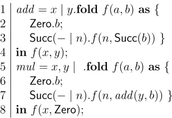
We briefly offer some intuition to the reader on the importance of opponent types and player types, and particularly how they interact to ensure that every well-typed function in Pola will halt in polynomial time. The matter will be discussed rigorously in section 3.4. Figure 3.3 gives two well-typed functions, add and mul, which naturally define ad-dition and multiplication on the natural numbers that were defined in figure 3.2. The

add function is exactly as it was defined in figure 3.2, where addition is performed via repeatedly taking the successor. Should we make a call to add(¯6,¯2), tracing through the recursive calls in the fold we find that we recurse 6 times, thus performing 6 Succ operations and ending up with a value of ¯8. The mul function is defined nearly identi-cally to the add function with three modifications: firstly, that the accumulated value begins at ¯0, as seen on line 8; secondly, and most importantly, that instead of repeatedly performing aSucc construction, the function repeatedly performs an addition operation; thirdly, the second parameter,y, is an opponent variable, not a player variable, which will be explained in the next paragraph. Consequently, should we make a call to mul(¯6,¯2), we would again recurse 6 times, performing 6 addition operations, each time adding ¯2, yielding a final value of 12.

The reason that the parameter y could be a player variable in the case of addis that

yis not used to drive a recursion. However, in the case of mul, the parameteryis used as the first argument to the functionadd, necessarily an opponent argument. The parameter

(35)

3.1. Introductory examples 25

1 exp =x, y | .foldf(a, b) as {

2 Zero.b;

3 Succ(− |n).f(n,mul(y, b)) }

4 in f(x,Succ(Zero));

Figure 3.4: A failed attempt at writing an exponential function in Pola. This example will lead to a typing error.

1 z =x| .fold f(x, y)as {

2 Zero.y;

3 Succ(− |n).f(n, f(n,Succ(y))) }

4 in f(x,Zero);

Figure 3.5: An exponential function which would yield a typing error in Pola.

this point that every formal parameter to a recursive function—i.e., the parameters a

and b in our example—is a player variable. Thus, attempting to rewrite the expression on line 7 to read f(n,add(b, y)) (puttingb in the first position of the addition) will yield a typing error as b is not an opponent variable but add’s first parameter is an opponent parameter.

If arithmetic is performed using the Peano representation of natural numbers given in figure 3.2, it must be impossible to write an exponential function. The reason is that computing an exponential using Peano arithmetic requires an exponential number ofSucc constructions. Figure 3.4 gives a natural attempt at writing an exponential function in Pola, following the style of arithmetic functions given in figure 3.3. If addition is iterated successors and multiplication is iterated addition, then exponential is iterated multiplication. The function in figure 3.4 yields a typing error: specifically, the mul

function requires both arguments to be opponent and, on line 3 of figure 3.4, the variable

b is a player variable. The typing system thus enforces that writing an exponential function in such a style is impossible. We will later prove that writing an exponential function is impossible in general.

Duplication of variables—that is, making reference to the same player variable more than once within a single evaluated term—in the player world is disallowed. Consider the program given in figure 3.5. The functionz would compute 2x₋_{1 and would operate}

in time exponential with respect to the size of x, due to the two recursive calls to f. This program would yield a typing error in Pola due to the fact that the variable n is duplicated. n is necessarily a player variable, because all recursive variables are player variables, and there is a general restriction on the duplication of any player variable.

There is one major exception to the restriction on duplication player variables just mentioned, which is that players may be duplicated between branches of a fold, an