Models of wet two dimensional foams

(1)

Models of Wet Two Dimensional

Foams

Friedrich Fionn Dunne

School of Physics

Trinity College Dublin

A thesis submitted for the degree of

Doctor of Philosophy

(2)

(3)

Declaration

I declare that this thesis has not been submitted as an exercise for a degree at this or any other university and it is entirely my own work. I agree to deposit this thesis in the University's open access institutional repository or allow the Library to do so on my behalf, subject to Irish Copyright Legislation and Trinity College Library conditions of use and acknowledgement.

(4)

(5)

Summary

In this thesis I used models and computer simulations to investigate the properties of two dimensional polydisperse foams from the dry limit of zero liquid fraction to the wet limit of 0.16 liquid fraction.

Initially I used the Plat software, which implements the standard model of two dimensional foams, to explore the full range of liquid fractions. As the software becomes increasingly less reliable towards the wet limit, we use over500,000 simulations in order to obtain results in this regime. We found the variation of energy and coordination number with liquid fraction, and the internal distribution of contacts in the foams.

We then focus on the variation of the coordination number with liquid fraction close to the wet limit. In particular, we compare the results of the Plat simulation with those of the Soft Disk model, which is widely used in the study of foams. The Soft Disk model is widely used due to its simplicity, but it is approximate, and neglects deformations.

A stark dierence between the two models is noted, with the Plat sim-ulation exhibiting a linear variation of the coordination number with liquid fraction, and the Soft Disk model exhibiting a square root variation.

(6)

the dierence in the variation of the coordination number. It appears to be due to the fact that the bubbles in the Plat simulation are deformable, while those in the Soft Disk model are not.

In order to explore the wet limit of two dimensional foams further, we develop a new model based on the theory of Morse and Witten. This model is dened for the wet limit, with deformable bubbles. It accurately predicts the response of a bubble of droplet to small deformations. We develop a framework and an algorithm for applying this theory to the case of modeling two dimensional foams.

The new simulation based on this model is tested against the Plat simu-lation. It produces comparable foams, with similar variations of the energy with liquid fraction. It also produces comparable contact changes with changes in liquid fraction. We propose an extension of this model to the case of three dimensional foams.

(7)

Acknowledgements

The most frequent reader of the start of a thesis is a new PhD student, so I want to begin mine with few words of encouragement to those setting o on their journey of discovery. I always knew that I wanted to study science, and to me, Physics gave the most fundamental explanations of how stu works. However, I never intended on doing a PhD, in school I always thought that that was solely for the best of the best. However, when I heard that Professor Stefan Hutzler had funding available for a PhD, I took a chance and went for it and here I am. If you have an idea, or see an opportunity, go for it! You never know what might happen.

I'd like to thank Stefan for taking a chance on me, and allowing me to turn his experimental PhD position into a computational one. None of this would have been possible without his enthusiasm, his tireless support, his hard work and dedication, and his passion for the eld of foams. I'd like to thank Professor Emeritus Denis Weaire for the clarity of his insight (both mathematical and physical), his font of research tangents that keep a project moving, and his constant demands for clearer explanations. I'd like to thank Professor Matthias Möbius for discussions of scaling laws, and the knowledge of when it's appropriate to use a log scale.

(8)

particular, the oce will be much quieter without you here. Jens, thank you for putting up with me getting you to double check my work all of the time. Both of you, thanks for making lunch so much more fun.

To my parents, thank you for encouraging me, supporting me, and simply for being proud of me. I love you both.

Becky, thank you for being patient with me through this. Without your kind and loving dedication this would not have turned out half as well as it did. (In particular, this thesis would be a lot poorer in commas!) Your encouragement and your belief in me mean the world to me. Simply put, I love you.

(9)

List of Publications

1. F. F. Dunne et al. Statistics and topological changes in 2D foam from the dry to the wet limit. In: Philosophical Magazine 97.21 (2017), pp. 17681781

2. J. Winkelmann et al. 2D foams above the jamming transition: De-formation matters. In: Colloids and Surfaces A: Physicochemical and Engineering Aspects 534 (2017). A Collection of Papers Presented at the 11th Eufoam Conference, Dublin, Ireland, 3-6 July, 2016, pp. 5257. issn: 0927-7757

3. Stefan Hutzler et al. A simple formula for the estimation of surface tension from two length measurements for a sessile or pendant drop. In: Philosophical Magazine Letters 98.1 (2018), pp. 916

4. B Haner et al. Ageing of bre-laden aqueous foams. In: Cellulose 24.1 (2017), pp. 231239

(10)

(11)

List of Tables

(16)

(17)

List of Figures

1.1 Everyday examples of foam . . . 2 1.2 Single layers of bubbles . . . 3 1.3 Close-up examples of wet and dry foam . . . 6 1.4 Schematic representation of the response of an elastic solid to

an applied shear stress . . . 12 1.5 An example of a Surface Evolver calculation of a bubble . . . 14 1.6 A Surface Evolver simulation of a junction between four Plateau

borders. . . 16 1.7 Illustration of the decoration of a dry Plateau border with

some liquid in two dimensions. . . 18 1.8 Illustration of the components of a T1 event . . . 19 1.9 Schematic of a single bubble in the standard model of two a

dimensional foam. . . 20 1.10 Comparison between Plat and the Soft Disk model. . . 22 1.11 Examples of bubbles in the Morse−Witten theory in two and

three dimensions. . . 26

(18)

2.2 The equilibrium condition for smoothly meeting arcs demands that θ1 =θ2 =π . . . 31

2.3 Variation of reduced excess energy, ε(φ), with liquid fraction, φ. . . 35 2.4 Coordination number Z versus liquid fraction φ. . . 37 2.5 Figure reproduced from [21] showing fractions of bubbles in

the foam with n contacts as a function of Z. . . 38 2.6 The fraction of bubbles with n neighbours as a function of

average coordination number, Z . . . 39 2.7 Example of a T1 transition where the average coordination

number,Z, is unchanged, but the distributionf(n)does change. . . . 40 2.8 The fraction of bubbles with n neighbours as a function of

liquid fraction, φ. . . 41 2.9 Distribution of number of sides of Plateau borders as a

func-tion of liquid fracfunc-tion. . . 42 2.10 Euler's equation versus average coordination number. . . 43 2.11 Two alternative illustrations of rearrangements due to a small

increase in liquid fraction. . . 45 2.12 Fraction of rearranged bubbles in a sample due to an increase

in liquid fraction by ∆φ as a function of liquid fraction φ. . . 46 2.13 Fraction of rearranged bubbles in a sample due to an increase

in liquid fraction by a range of ∆φ values, each as a function of liquid fraction φ. . . 48 2.14 Log-linear plot of histograms of the fraction of bubbles

[image:18.595.137.514.125.544.2]

(19)

2.16 Comparison of Z(φ) data between Plat simulations and Soft Disk model results. . . 54 2.17 The radial density function, g(r), gives the probability of two

disk centers being a distance r apart. . . 57 2.18 Interpartical distance measurements for calculating g(r). . . . 58 2.19 An illustration of the separation, w, between bubbles in two

dierent models . . . 59 2.20 Distribution of separations, f(w), a for two dimensional foam

and a two dimensional disk packing at a similar average coor-dination number ZSD= 4.07±0.01 . . . 61

3.1 Shear modulus, G, versus excess packing fraction, δφ, repro-duced from [82]. . . 69 3.2 Prole of the solution to the linearised Young−Laplace

equa-tion according to Morse and Witten . . . 73 3.3 The shape of the two dimensional Morse−Witten prole given

by Equation (3.13). . . 76 3.4 The shape of a two dimensional bubble trapped between two

parallel lines . . . 78 3.5 Two dierent sized two dimensional bubbles held in contact

with each other by opposed body forcesF, as calculated using Equations (3.2) and (3.13). . . 80 3.6 Sequence of bubble positions illustrating the procedure used

to numerically measure centre−centre distance as a function of contact force magnitude. . . 82 3.7 Dimensionless change in separation versus force between two

(20)

3.8 The prole of a two dimensional Morse−Witten bubble re-sulting from the linear combination of the individual proles associated with each of the four contacts. . . 84 3.9 Iteration scheme for the computation of a two dimensional

Morse−Witten foam. . . 89 3.10 A semi-logarithmic plot of the maximum net force as a

func-tion of iterafunc-tion number for a test simulafunc-tion of ten bubbles. . . . 91 3.11 An example of a ten bubble simulation that did not approach

convergence. . . 92 3.12 Comparison of a polydisperse two dimensional foam as

com-puted using the Plat simulation software and the Morse−Witten formulation. . . 93 3.13 The coordination number of the two foam simulations depicted

in Figure 3.12 as a function of φ. . . 94 3.14 Example of a 100 bubble simulation at φ= 0.13. . . 96 3.15 Variation of normalised excess energy as a function of∆φ=

φc−φ). . . 97

3.16 Force network in Morse−Witten simulations . . . 99

4.1 Examples of a pendant and sessile drop. . . 105 4.2 Examples of proles of sessile and pendant drops, computed

by integrating the Young−Laplace equation. . . 108 4.3 Examples of proles of sessile and pendant drops, obtained

from the result of Morse and Witten. . . 110 4.4 Variation of the dierence of our two length measurements

(Lx−Ly) as a function of their sum (Lx +Ly) for numerical

(21)

4.5 A dimensionless plot of the data in Figure 4.4. . . 115 4.6 Sample pendant drop image from Berry et al. [103] . . . 116 4.7 Example of a pendant drop. . . 116

5.1 An illustration of the large arc - small arc ambiguity in the Plat simulation. . . 120 5.2 Survival and mortality of Plat simulations as a function of

liquid fraction. . . 122 5.3 PreliminaryZ(∆φ)data for the two dimensional Morse−Witten

(22)

(23)

Chapter 1 What is a Foam?

Most generally, a foam is considered to be a two-phase system of gas bubbles dispersed within a liquid. Foams are a part of everyday life, sometimes benecial, other times a nuisance, but mostly we don't give foam a second thought. Whether it's a squirt of shaving foam (which doesn't ow o skin under gravity) in the morning, the white head creating the creamy texture of a pint, or a pot of pasta boiling over, foam is everywhere. Industrial processes which make use of foams include foam fractionation for water treatment and froth otation for mineral separation in mining [6]. Also studied in conjunc-tion with foams are other two-phase systems such as emulsions, which consist of one immiscible liquid dispersed within another. Foams and emulsions have very similar physical properties. In this thesis reference will only be made to foams, without loss of generality the simulations and results can also be applied to emulsions.

(24)

(a) Shaving foam (b) A creamy pint Figure 1.1: Everyday examples of foam

drains out of the lms, causing the bubbles to burst. Bubbles collect and build up into a foam when there are additives, such as soap or proteins, in the liquid that can stabilise the lms and prolong the lifetime of the bubbles. Surfactants are a class of molecules to which soaps belong. These are undecided molecules which have parts that energetically favour being in water and parts that do not. Due to this, they place themselves at interfaces, where both their parts can be satised. There they lower the surface tension and, thanks to gradients in their concentration, they can stabilise the thin lms that separate the air pockets, preventing rupture. How surfactants act and how their properties inuence those of the foam is a subject of ongoing research [7, 8], but outside the scope of this thesis.

1.1 What are Two Dimensional Foams?

(25)

[image:25.595.159.395.127.392.2]

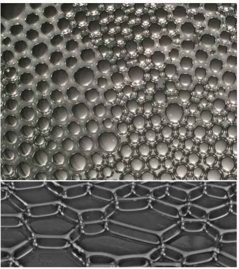
Figure 1.2: Top: A close up of a single layer of bubbles (diameter ' 0.5 mm)

oating on a liquid pool (an example of a Bragg raft). Image credit: Steven Burke, TCD Foams group. Bottom: A close up of a single layer of bubbles (diameter'1 cm) sandwiched between two glass plates separated by3 mm(an

example of a Hele-Shaw cell). Image credit: Benjamin Haner, TCD Foams group

regular three dimensional bubbles in one of three congurations: between two parallel (transparent) plates (also called a Hele−Shaw cell [9]), oating on top of a liquid reservoir (also called a Bragg raft [10]), or oating on a liquid reservoir with a covering transparent plate pressed down on top. They are called quasi-two dimensional because there is a three dimensional liquid network surrounding the bubbles in the monolayers [11].

(26)

bubble in two dimensions. For example, a two dimensional foam may be sheared to measure its ow behaviour while being imaged to track the motion of individual bubbles [12]. This is very dicult to do in three dimensions, where simple imaging techniques fail due to the scattering of light as the light passes through multiple interfaces. Therefore, in three dimensions, expensive and cumbersome x-ray equipment is needed in order to see into the centre of a foam.

Another area that is much more accessible in two dimensions is simu-lation. A simulation in two dimensions is computationally quicker than in three dimensions because there are fewer interactions to calculate. This can be understood from the fact that, in a simple three dimensional cubic lattice there are 26 (3D=3 ₋ ₁₎ _{next nearest neighbours, compared to only eight}

(3D=2₋₁₎_{in two dimensions. This is compounded by the fact that, for a three}

(27)

1.2 Properties of Foams

1.2.1 Liquid Fraction

A simple property of a foam that can be considered is its global liquid fraction, φ [13]. This is the ratio of the total liquid volume to the total foam volume. Foams with a liquid fraction below ∼ 0.10 are considered dry foams, with polyhedrally shaped bubbles (see Figure 1.3 (top)). Foams with higher liquid fractions are considered wet foams, with roughly spherically shaped bubbles (see Figure 1.3(bottom)). The distinction between wet and dry foams is they have both dierent geometries and they both exhibit dierent behaviours due to the dierent overall bubble shapes (see Section 1.2.5 for examples to do with ow behaviour).

The Dry Limit

Very dry foams (with a liquid fraction below 0.01) can be described as a collection of thin lms of negligible thickness around a cellular structure of gas bubbles in (roughly) polyhedral shapes, though the interfaces are in general curved, as described by the YoungLaplace law (see Section 1.3.2.

The Wet Limit

There is a particular value of liquid fraction, φc, know as the critical liquid

(28)

[image:28.595.160.475.197.561.2]

Figure 1.3: Close-up examples of a dry foam (φ <1∼2%) (top), and a wet foam

(φ _' 20 _∼ 25%) (bottom). Bubbles in the dry foam are mostly polyhedral,

(29)

since, close to this value of φ, other properties of foams exhibit interesting scaling laws [14]. Some of these will be discussed in Sections 1.2.3 and 1.2.4. At φc in three dimensions, a foam closely resembles a granular packing

of hard spheres, while in two dimensions, it is quite similar to a packing of hard disks. φc for a polydisperse foam (with a range of bubble sizes, see

Section 1.2.2) in three dimensions is 0.36, while in two dimensions it is 0.16. This is due to the fact that disks ll a two dimensional plane more eciently than spheres ll a three dimensional space.

1.2.2 Bubble Sizes

When studying foams under gravity, a natural length scale arises from con-sidering the competition between gravity pulling the liquid out of the lms and surface tension pulling the liquid back into the lms. This is called the capillary length

λc =

r _γ

ρg, (1.1)

whereγ is the surface tension, ρ is the liquid density, andg the acceleration due to gravity. This length tells how far water will be drawn up into the foam by capillary action. Typical water and soap solutions have a density of 1000 kg m−3 _{and a surface tension of} _{25 mN m}−1 _giving _λ

c = 1.6 mm. This

can be compared to the typical bubble sizes in a foam.

One possible measure of the size of a bubble is given by its equivalent sphere radius R. That is, the radius of a sphere with the same volume as the bubble. These vary widely depending on the foam and can range from less than a millimetre up to a metre [15], so can be smaller or larger than the capillary length. Film thicknesses may be in the range of5 nm to10µm, much smaller than the capillary length.

(30)

This generally does not occur in nature where random processes are usually at play, but the simplicity it aords makes it useful in the lab. Additionally, using monodisperse liquid foams as a precursor to solid foam materials gives a way to nely control the structural properties of these materials [16]. The bubbles in a monodisperse foam can tend to form an ordered, crystalline structure. When the bubbles come in a range of sizes the foam is termed polydisperse. The polydispersity is measured as the standard deviation of the distribution of radii divided by the average bubble radius, dened in terms of the mean (hRi) and squared mean (hR2_{i) of the distribution of} _R

as

σR =

s

hR2_i

hRi2 −1. (1.2)

For a perfectly monodisperse foamσR = 0, but for practical purposes a foam

is considered to be monodisperse if σR < 0.05. In contrast to monodisperse

foams, a polydisperse foam forms disorded, random structures. Polydisperse two dimensional foams are found to crystallise, at least partially, forσR <0.1,

and form truly random systems when σR > 0.1 [17]. In the intermediate

range of 0.05 < σR < 0.1, foams tend to form partially crystalline systems,

with localised regions or order and disorder. Another way to create disor-dered, random structures is to mix two monodisperse foams with dierent bubble sizes. The result is called a bidisperse foam. In bidisperse foams the critical size ratio of large bubbles radius to small bubble radius need to form disordered structures is 1.14 [18]. The order and disorder, i.e. the respective presence or absence of long range correlations in the bubble positions, in a foam can greatly inuence its properties. For example, in two dimensions an ordered monodisperse foam has a φc= 1−π/(2

√

(31)

1.2.3 Energy

In the standard quasi-static models of foams (see Section 1.4.1 for two di-mensional examples), the gas in the bubbles is treated as incompressible; therefore, the surface energy is the only relevant energy for describing the two dimensional foams. The surface energy of a foam is E =γA, where A is the total surface area. In the case of two dimensional foams, the equivalent of the surface energy is then a line energy, proportional to the total perimeter of all the bubbles.

A foam will adopt a conguration which minimises this energy. Therefore, the lms in a foam fall into a category know as minimal surfaces, a local minimum. To globally minimise their energy, the lms would collapse into a single disk of liquid. This does not happen if the local minimum is stable enough (i.e. the lms don't burst). A corollary of this is that a bubble that is free to move will always form a sphere in three dimensions, or a circular disk in two dimensions. Note that, in the models described here it will always be assumed that the lms will not burst.

At all values of liquid fraction below the critical liquid fraction (φ < φc),

the bubbles are deformed from spherical, increasing their surface energy. Therefore, a dimensionless excess energy can be dened as

ε(φ) = E(φ)−Ec Ec

= E(φ) Ec −

1, (1.3)

where Ec=E(φc), the energy of the foam in the wet limit.

1.2.4 Coordination Number

(32)

otherwise stable conguration. These, therefore, do not contribute to the mechanical stability of the foam, and thus do not contribute to many of the physical properties of the foam. In two dimensions these loose bubbles, known as rattlers, can be identied by the fact that they have less than three contacts each (less than four each in three dimensions) and, thus, cannot be mechanically stable. The coordination number, Z, of a foam is the average number of contacts per bubble, after these rattlers have been discounted. This does not aect the coordination number signicantly as the rattlers make up at most 2% of the bubbles (see Chapter 2, Figure 2.6 for more details). For a polydisperse, disordered foam, this is a function of liquid fractionφ. Generally, in two dimensions, the distribution of contact numbers appears to follow a Gaussian distribution with a xed width, regardless of the model used to simulate the foam (see Section 2.2.4).

The value ofZ in the dry limit can be shown to be six via Euler's theorem which relates the number of faces, edges, and vertices of a cellular structure to a topological invariant (see [15] for a detailed explanation).

At the wet limit, φc, the limiting value of the coordination number,

Z(φc) = Zc, can be found by looking at degrees of freedom. For each

dimen-sion in a given model or experiment, a bubble has one degree of freedom. In the wet limit there are just enough constraints on the foam that each bubble is held in place. Each contact provides one constraint to two bubbles. This leaves each bubble with, on average, Z/2 constraints. Equating degrees of freedom with constraints, we get3 = Zc/2in three dimensions and2 = Zc/2

in two dimensions. Therefore, on average in an system of innite size,Zc= 6

in three dimensions, and Zc= 4 in two dimensions [19, 20, 14].

(33)

conditions and N bubbles, the system does not change if we move every bubble by the same amount (it is invariant under translation). This means that one bubble can be xed (equivalent to xing a point of view), leaving 2(N−1)degrees of freedom. Equating this to the N Zc/2constraints we get

Zc= 4(1−1/N). As we increaseN we can see that the correction for nite

size vanishes.

Various experiments for quasi-two dimensional foams [21] and two di-mensional elastic disks [22], and simulations with the more approximate Soft Disk model [23] have been in agreement in nding the limiting form for the average coordination number Z. In particular,

Z−Zc∝(φc−φ)1/2, (1.4)

where Zc=Z(φc).

The discovery of the square root scaling for Z(φ)appears to date back to the work of Durian using the so-called Soft Disk model (see Section 1.4.2 for details). Durian developed this model primarily to investigate the rheological properties of foams, of which it indeed provides a good overall description [24, 25, 26]. Two dimensional bubbles are approximated as disks, subject to repulsive forces when they overlap.

The same square-root scaling for Z(φ) was also found in computer simu-lations of packings of three dimensional soft spheres [27], a system which has since been called the Ising model for jamming [14].

(34)

l

[image:34.595.232.411.133.267.2]

∆l τ

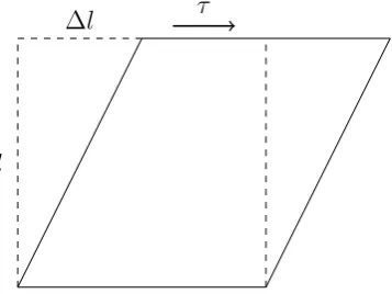
Figure 1.4: Schematic representation of the response of an elastic solid to an applied shear stress, τ. The dashed lines represent the undeformed solid, the

solid sloped lines represent the solid's response to the strainτ. ∆lmeasures the

deformation of the solid, which has a heightl, thus the resulting strain is ∆l/l.

1.2.5 Rheological Properties

When an elastic solid is subjected to a small shear stress, τ, as depicted in Figure 1.4, the relative deformation, or strain,∆l/l is linearly related to the applied stress by the shear modulus, where ∆l is the change in length and l is the width. Foams behave like elastic solids when a small stress is applied. When the stress on a foam is increased it will reach a critical point after which the foam will not deform like an elastic solid, but it will ow like a liquid. The amount of stress required to get a foam to start owing (i.e. in continuous motion with bubbles constantly rearranging) is called the yield stress,τy.

A liquid deforms continuously under an applied stress. The strain rate, ˙

(35)

in a foam, the resistance to ow is amplied by this same factor. This means that the eective viscosity of a foam is typically at least 104 _{times greater}

than that of the liquid in the foam.

Additionally, the relationship between stress and strain rate is no longer linear. Firstly, the strain rate is zero for any stress below the yield stress. Secondly, the relationship between stress and strain rate in a foam is in fact

τ =τy +κγ˙n, (1.5)

a power law know as the Herschel−Bulkley [28] law. Here, κ can no longer be called a viscosity as its dimensions must change to compensate for the eect the power n has on the dimensions of γ˙. Instead it is referred to as the consistency, but it plays the role of an eective viscosity. As our models are quasi-static rather than dynamic, the details of rheology, the study of ow, will not form part them. However, we will still be able to predict some properties that can be related to the rheology of foams.

Wet foams, with higher liquid content, ow much more easily than dry foams. This is because as φ is increased towards φc, the area of the lms

between contacting bubbles decreases. This makes it easier for bubbles to rearrange, and as a result, both the shear modulus and the yield stress of foams decrease as the liquid content of the foam is increased. Beyondφc, the

(36)

CHAPTER 1. WHAT IS A FOAM?

Z

-cone model for the energy of an ordered foam

Stefan Hutzler,* Robert P. Murtagh, David Whyte, Steven T. Tobin

_†

and Denis Weaire

We develop the

Z

-Cone Model, in terms of which the energy of a foam may be estimated. It is

directly applicable to an ordered structure in which every bubble has

Z

identical neighbours. The energy

(

i.e.

surface area) may be analytically related to liquid fraction. It has the correct asymptotic form in

the limits of dry and wet foam, with prefactors dependent on

Z

. In particular, the variation of energy with

deformation in the wet limit is consistent with the anomalous behaviour found by Morse and

Witten [

Europhysics Letters

, 1993,

22 , 549] and Lacasse

et al.

[

Physical Review E

,

54 , 5436], with a

prefactor

Z

/2.

1 Introduction

Many of the physical properties of foams may be understood in

terms of the minimisation of surface area, under appropriate

constraints. This is the condition for static equilibrium, since

total energy is proportional to surface area if gas and liquid are

treated as incompressible.

Brakke's Surface Evolver

1

_{provides a practical method to}

compute such equilibrium structures, represented by



nely

tessellated surfaces. It is natural to seek simpler representations

and models to provide estimates of energies and forces, even at

the expense of drastic approximations, such as pairwise

inter-action potentials between bubbles.

2,3

This has raised a number of questions, addressed by Morse

and Witten

4

_{and Lacasse}

_{et al.}

5

_{How valid is the assumption of}

pairwise additive potentials? What is the true form of interaction

(

i.e.

the change in surface area) between two bubbles

which barely touch each other? We o

ﬀ

er a new approximate

formulation, the

Z

-Cone Model, that advances our understanding

of such questions, in terms of analytic solutions of the model.

As in the work of Lacasse

et al.

, we consider a foam in which

each bubble has

Z

equivalent neighbours, for example the

face-centred cubic structure (

Z

¼

12). We seek to evaluate the energy

(or surface area) as a function of

Z

and the degree to which the

bubbles are compressed together (that is, the liquid fraction).

Both gas and liquid are treated as incompressible.

Our essential geometrical approximation is inspired by

Ziman's early description of the Fermi surface of copper.

6

The

bubble volume can be divided into

Z

equivalent objects

which meet at a central point. We take one such object and

approximate it by a cylindrically symmetric cone of the same

solid angle and volume, as shown in Fig. 1. Note that these new

cones, if assembled, would

‘

overlap

’

since cones cannot tile 3D

space.

The equivalence of the

Z

sections corresponds to a regular

polyhedron in the dry limit; such regular polyhedra have been

the starting point for theories of dry foams.

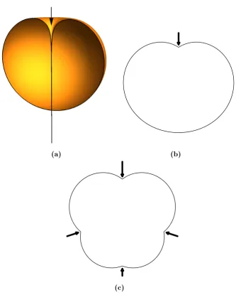
7

Fig. 1

The shape of a bubble in a crystalline foam with

Z

equivalent

neighbours, shown in (a) for

Z

¼

12, may be approximated by an

assembly of

Z

cones of the type shown in (b). Its

ﬂ

attened surface

corresponds to a bubble

–

bubble contact. (c) 2D cross-section of a

cone with relevant notation. During bubble deformation, total

bubble volume

V

and total solid angle must be conserved, according

to

V

¼

ZV

c

and 4

p

¼

Z

U

, where

V

c

¼

2

3 p

R

0

3

_ð

₁

_cos

_q

_Þ

_{is the volume}

of a cone with opening angle

q

¼

arccos(1

2/

Z

),

R

0

is the radius of the

spherical sector (corresponding to an undeformed cone) and

U

is the

solid angle of the cone.

School of Physics, Trinity College Dublin, Dublin, Ireland. E-mail: stefan.hutzler@tcd.ie

†

Present address: University of Melbourne, Melbourne, Australia.

Cite this:

Soft Matter

, 2014,

10 , 7103

Received 9th April 2014

Accepted 1st July 2014

DOI: 10.1039/c4sm00774c

www.rsc.org/softmatter

Soft Matter

PAPER

Published on 03 July 2014. Downloaded by Trinity College Dublin on 10/22/2018 3:55:31 PM.

View Article Online

View Journal | View Issue

Figure 1.5: An example of a Surface Evolver calculation of a three dimensional bubble with 12 symmetric contacts in an ordered, monodisperse foam by Hutzler et al. [38]. The dashed lines on the faces indicate the boundaries of the contact faces when this single bubble is repeated to represent a crystalline foam.

Hutzler et al. [36].

1.3 Describing Foams

1.3.1 Minimal Energy Surfaces

We can completely describe a foam if we can fully describe the position and shape of all of its lms. Finding the lm conguration that minimises the surface energy can, in general, only be done numerically. For this task, a software called Surface Evolver is commonly used [37]. It is a program which, when given an initial surface, will minimise its energy, subject to constraints. There are many situations where the minimal energy condition is su-cient for calculating the conduration of a foam, particularly if there is a

(37)

high degree of symmetry involved (see for example Figure 1.5). To aid our understanding of foams, additional rules about the shapes and interactions of lms in foams can be derived from this condition.

1.3.2 YoungLaplace Law in Three Dimensions

Each gas-liquid interface has a pressure dierence, ∆p, across it, and so its curvature is given by the Young−Laplace law

∆p= 2γ

r (1.6)

whereγ is the surface tension andrthe mean local radius of curvature. This mean local curvature is related to the two principle curvatures of the surface, r1 and r2, by

1 r =

1 2

1 r1

+ 1 r2

. (1.7)

A single gas bubble in a liquid is a sphere, and so only has one principle curvature everywhere (r = r1 =r2). A bubble in air, as a child would blow

with a bubble wand, has two liquid−gas interfaces. This eectively doubles the surface tension and the radius. This is because a higher surface tension makes deforming the interface more costly in terms of energy.

(38)

1.3.3 Plateau's Laws for Dry Foam in Three Dimensions

4864 S J Coxet al

δ

[image:38.595.205.429.175.393.2]

L

Figure 1.A single tetrahedral junction of Plateau borders. The radius of curvature of the Plateau borders is equal toδ(as lengthL→ ∞).

In practice v is often measured as the velocity of the front of the solitary wave that is

generated when a given flow is first imposed on the dry foam. The earliest experiments of this

kind [9] established a scaling law betweenv andQ:

v ∝Q1/2 ₍₂₎

where the exponent was established to within about ten per cent. This result, later confirmed for various detergent systems [10, 11] and protein foams [12, 13], was the spur to subsequent theoretical analysis. The foam drainage equation based on Poiseuille flow was found to be consistent with (2).

However, fresh experimental results obtained in 1999 [1] lead to a reappraisal of the model. The new data, which were of greater extent and precision than previous results, indicated a different power law:

v ∝Q1/3_. ₍₃₎

Koehleret al showed this to be consistent with an alternative model in which dissipation is

dominated by the vertices or nodes where the Plateau borders meet. The implication is that there is plug flow rather than Poiseuille flow in the borders themselves.

While the earlier conclusions were based on data of a lesser accuracy, they had been independently confirmed many times. There was therefore a sharp conflict of evidence, which was soon resolved by the realization that different surfactants were used by the two groups [5]. The new experiments used the commercial detergent Dawn whereas the earlier work used (mostly) Fairy Liquid. Not all dishwashing detergents are the same!

On closer examination, most of the experimental results deviate somewhat from the ideal values 1/3 and 1/2 for the index which is at issue. They mostly lie between these extremes. This calls for a combined model [12, 14], and indeed further experimentation on a wide range of surfactant systems which are better defined.

Now that the vertices are seen as important, it is useful to calculate the flow properties associated with them. Here we present numerical calculations for the two limiting cases—

Figure 1.6: Figure reproduced from [40]. A Surface Evolver simulation of a junction between four Plateau borders. This shape is dicult to describe ana-lytically, but the result of numerical calculations such as this one provide a lot of information, such as how the width of the plateau border, δ, changes with

proximity to the node, L.

If we consider lms with negligible thickness (i.e. in the dry limit) then the meeting of these lms is governed by Plateau's laws. The rst of these states that the meeting of lms occurs in threes and, being symmetric, they meet at120◦. The lines along which the lms meet are called Plateau borders. When the liquid content of a foam is increased, these thicken into channels. The second rule governs the meeting of these Plateau borders and states that they meet in groups of four, and at equal angles. These meeting points are called nodes. When the liquid content of a foam increases, they can take on complex shapes and can be dicult to describe analytically [15]. Figure 1.6

(39)

shows a Surface Evolver calculation of the shape of a node. These laws are a consequence of the energy minimisation of the lms.

1.3.4 YoungLaplace Law in Two Dimensions

As discussed in Section 1.1, two dimensional foams are often used to study complicated phenomena in real foams in a simplied setting. In this case, the gas-liquid interfaces are lines instead of surfaces. Therefore, there is only one principal radius of curvature, r, per interface, and the Young−Laplace law simplies to

∆p= γ

r. (1.8)

This has the implication that each segment of a bubble's boundary, be it a bubble−bubble or bubble−liquid interface, is described by an arc of a circle of radius given by Equation (1.8). At contacts with neighbouring bubbles there are two liquid−gas interfaces, one for each bubble. To account for this we use twice the surface tension in determining the curvature of these edges, compared with the regular bubble−liquid interfaces.

1.3.5 Plateau's Laws in Two Dimensions

(40)

(a) Dry Plateau border (b) Wet Plateau border

Figure 1.7: Illustration of the decoration of a dry Plateau border with some liquid in two dimensions. The wet Plateau border (b) is still a threefold meeting of edges and at each corner of the Plateau border the lines meet smoothly.

[30]. When the amount of liquid exceeds 0.05, the condition of meeting in threes is relaxed and Plateau borders begin to meet and join together. This will be shown in more detail in Section 2.2.5.

1.3.6 Topological Changes in Two Dimensions

When two Plateau borders, with three sides each, come into contact they merge into a four-sided Plateau border. For very dry foams, φ < 0.05, a four-sided Plateau border is unstable and will revert back to two three-sided Plateau borders, but with the opposite orientation to the original pair, see Figure 1.8. This is termed a topological transition of the rst kind by Bolton and Weaire [31], or a T1 for short. Since the total number of contacts does not change in a T1, the average coordination number cannot change through these events. Only once the four-sided (and larger) Plateau borders become stable can bubbles lose contacts and the coordination number decrease.

(41)

1

2

3 4

1

2 3 4

1

2 3 4

Figure 1.8: Illustration of the components of a T1 event. Two three-sided Plateau borders merge to form an unstable four-sided Plateau border. This in turn decays into two three-sided Plateau borders, but with the orientation perpendicular to the original pair.

Therefore, we study simply the individual contact changes in the foam, rather than T1 events. To study just the contact changes we can make use of an idea from graph theory called the adjacency matrix. This is a squareN ×N matrix of zeros and ones whose elements ij equal to one if bubble i is in contact with bubblej, and zero otherwise. Simply by subtracting successive matrices, changes in the contact network show up as non zero elements in the dierence. I have used this approach to study rearrangements in two dimensional foam simulations in Section 2.3.

1.4 Modelling Two Dimensional Foams

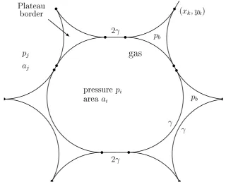
1.4.1 Standard Model of Two Dimensional Foams

(42)

2γ 2γ pj

aj

(xk, yk)

pressure pi

area ai

gas

γ γ pb

pb

[image:42.595.157.478.130.395.2]

Plateau border

Figure 1.9: Schematic of a single bubble in the standard model of two a dimen-sional foam. (xk, yk)is the position of vertexk,γ the interfacial surface tension,

pb the Plateau border pressure,pi the gas pressure of bubblei, and ai the area

of bubble i.

area. The lms between contacting bubbles are assumed to have negligible thickness. The curvature of each lm is determined by Equation (1.8).

(43)

interface so the surface tension used is half that of the lms.

The corners of the Plateau borders are called vertices. At each vertex, two liquid−gas interfaces meet one lm. They must all meet smoothly, i.e. their tangents much be equal at the vertex. This is the extension of Plateau's law into wet two dimensional foams.

These conditions are sucient to fully describe any two dimensional foam. One implementation of this model is a software program called Plat, intro-duced in the early 1990s by Bolton and Weaire [30, 31, 32, 33]. It has been used extensively in this thesis and will be covered in further detail in Section 2.1.1. It is a quasi-static model producing two dimensional foam structures which satisfy Plateau's laws. The Plat simulation is very reliable for dry foams and moderately wet foams, but unfortunately less so for very wet foams (φ & 0.12), see Section 5.1.2 for detailed statistics. For systems with over 20 bubbles it can fail to nd an equilibrium conguration at liquid fractions beyond 0.1, with the probability of failure increasing with both system size and liquid fraction.

(44)

this is quite similar to real foams, it does not represent the idealised case of zero contact angle which is used to study foams theoretically.

1.4.2 Soft Disk/Sphere Model

In the wet limit of two dimensional foams, the bubbles are all circular. In fact, foams in the wet limit can be described as packings of hard disks, as discussed in Section 1.2.1. This led to the development of the Soft Disk model in which bubbles are approximated as circles. Away from the wet limit the disks are allowed to overlap. When the disks overlap they repel via a simple potential, often approximated as harmonic [34]. This has been chosen mainly for computational simplicity. However, Surface Evolver simulations have shown that, while the energy is harmonic in two dimensions, the bubble-bubble interactions are not pairwise-additive [46]. That is, the model of interaction that lies at the heart of the Soft Disk model does not represent realistic bubble-bubble interactions. This will be addressed in Chapter 3.

(a)

pb

pressurepi

pj (b)

Figure 1.10: Comparison between Plat and the Soft Disk model for φ = 0.90.

(45)

Additionally, the Soft Disk model does not conserve gas area, while the Plat implementation of the standard model of two dimensional foam does. This is immediately apparent when considering visual representations of Plat (Figure 1.10(a)) and the Soft Disk model (Figure 1.10(b)).

An associated diculty is the denition of liquid fraction in the Soft Disk model. The liquid fraction in the standard two dimensional model is readily dened as the fraction of the whole simulation geometry not lled with bubbles. With the overlapping disks in the Soft Disk model it becomes quite dicult to calculate the area of each overlap when more than two spheres partially overlap the same area. Computationally this would also defeat the purpose of the simplicity of the model. Instead, in the spirit of a rst order approximation, the double counting of the overlap areas is simply ignored, and the liquid area is calculated as the whole simulation area minus the sum of the disk areas. For more compressed (i.e. dry) cases this can lead to negative liquid fractions, a physical impossibility. Of course, the model is dened in the wet limit and so should not be expected to produce sensible results for dry foams.

In three dimensions an analogous model is used called the Soft Sphere model. It treats the bubbles as spheres that are allowed to overlap. When they overlap, they repel with a harmonic potential. In both the two and three dimensional cases, part of the success of the model can be attributed to the fact that the harmonic potential is arbitrary and may be tuned to model one specic experiment.

While this has been successful in reproducing the Herschel−Bulkley type rheological behaviour that is associated with emulsions and foams, it does not reproduce all of the behaviours of foams.

(46)

to being close to the wet limit) is intrinsically anharmonic [47]. This anhar-monic nature was identied by Morse and Witten [48] and has resulted in a model which will be outlined in Section 1.4.3.

1.4.3 MorseWitten Model

One of the main issues with the Soft Disk model is that it does not conserve bubble area as it does not allow bubbles to deform. The Plat implementation of the two dimensional foam model does conserve area and allows bubbles to deform, but it fails in the wet limit. Therefore, we wish to create a two dimensional model for foams which combines some of the simplicity of the Soft Disk model with deformable bubbles away from the wet limit.

To do this we turn to the work of Morse and Witten [48]. The result of that work is a relationship between an applied force on a bubble and the deformation of the bubble in response. Morse and Witten obtained an expression for the deformation of a bubble from spherical, shown in three dimensions in Figure 1.11 (a) and in two dimensions in Figure 1.11(b). Also shown in Figure 1.11(c) is the response of a bubble to several applied forces. A main result of this is that the interaction between three dimensional bubbles is logarithmically soft for small deformations, much softer than a harmonic interaction. This non-linear scaling is weaker than the Hertzianf−1/3_{seen for}

contacting elastic solids [49], but it still dominates the energetics of weakly compressed foams.

(47)

(48)

(a) (b)

[image:48.595.149.483.120.536.2]

(c)

Figure 1.11: Examples of bubbles in the Morse−Witten theory in two and three

dimensions. (a) A slice through a three dimensional Morse−Witten bubble

(49)

Chapter 2 Studying Two Dimensional Foams

with Plat

(50)

brute force approach in order to explore the wet limit.

Before detailing the workings of the Plat simulation, I will revisit other critical phenomena that two dimensional foams have been found to exhibit in the wet limit. Following this, I will detail how Plat implements the stan-dard model of two dimensional foams, along with the procedure used in the simulations. The rst data analysed will be the variation of energy and of the coordination number with liquid fraction to complement previous work. Subsequently, the occurrence of cascades of bubble rearrangements in the wet limit is analysed. The coordination number variation provided some results that contrast with much of the literature so that will then be revisited and compared in detail with results from the soft disk model. This will show that the deformation of the bubbles due to area conservation plays an important role. This was our main motivation to develop the Morse−Witten model for two dimensional foams, as will be described in Chapter 3.

2.1 The Plat Software

2.1.1 Details of the Implementation

Plat, as mentioned in Section 1.4.1, is a software package for the simulation of a foam in two dimensions. It is based on the direct implementation of Plateau's Laws, rather than an energy minimisation routine.

(51)

[image:51.595.138.418.125.643.2]

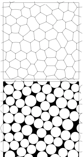
Figure 2.1: Example of initial (dry,φ= 0.002) and nal (wet, φ= 0.165) stages

(52)

in the simulation box. (The randomness of bubble areas is controlled by specifying a minimum separation between points, the so-called hard disk parameter as described by Weaire and Kermode [51]. A lower minimum separation results in greater polydispersity.) These points are then connected into a triangular tessellation of the box. The denition of the tessellation is used to connect the random points together.

Next, the Delauney tessellation is inverted to obtain its dual graph, a Voronoi network. In this transformation, the random points used as the corners of the triangles become the centres of the Voronoi cells. It is these cells that represent the bubble in the simulation. The circumcentres of each triangle become the corners of the Voronoi cells. Once the transformation is complete, the resulting Voronoi network is converted to a relatively dry foam (φ <0.002), not yet equilibrated, by decorating its vertices with small three-sided Plateau borders at equal pressures. This initialisation procedure is provided by Plat and is based on the procedure described by Kermode and Weaire [52].

The decorated Voronoi network is equilibrated into a two dimensional foam by adjusting cell pressures and vertex coordinates in order to full the constraints of xed cell areas and smoothly meeting arcs. The cell pressures are updated by

∆pi =−

γA∆Ai ∂Ai

∂pi

, (2.1)

where ∆Ai is the existing discrepancy of the current cell area from the true

area, ∂Ai

∂pi is the numerically determined area derivative, andγAis a damping factor required to stabilise the algorithm. The cell pressures change the cell areas by controlling the boundary curvatures. This step is repeated until the xed cell areas are correct.

(53)

θ2

θ1

Figure 2.2: The equilibrium condition for smoothly meeting arcs demands that

θ1 =θ2 =π

at each vertex. In this way, the conditions of the standard two dimensional foam model (Plateau's laws and the Young−Laplace law) are fullled (see Section 1.4.1). The increments(∆xk,∆yk) are calculated via





∆xk

∆yk



=γθ

  ∂θ1 ∂xk ∂θ1 ∂yk ∂θ2 ∂xk ∂θ2 ∂yk  

−1 

π−θ1

π₋θ2



, (2.2)

where the anglesθ1 andθ2 are as in Figure 2.2, the derivatives are calculated

numerically, and γθ is a damping factor. This process is repeated until the

largest vertex increment falls below a convergence threshold. The threshold is an adjustable fraction of the average Plateau border radius, defaulting to 0.02. See also [31] for a detailed discussion of the Plat representation of a foam and the equilibration process.

There are two types of topological changes implemented during equilibra-tion. These correspond to the two components of a T1 change (Section 1.3.6). Cells lose contact when the vertices at either end of their shared cell−cell boundary come within an adjustable fraction (defaulting to 0.01) of the average radius of a Plateau border of each other. Cells come into contact when their corresponding cell−border arcs overlap across a Plateau border.

(54)

network and can be dealt with easily. Even towards the wet limit, the fraction of bubbles with just one or two contacts combined is less than 4% (see Section 2.2.4).

2.1.2 Simulation Procedure

The simulations presented here progress by increasing the liquid fraction in steps of ∆φ = 0.001 and equilibrating the foam at each step. Increases in liquid fraction are performed by proportionally reducing bubble areas (rather than increasing the total simulation area). This involves decreasing the cell pressures in order to reduce the curvature of the liquid−gas interfaces, followed by the equilibration of vertex positions. The change in pressure of every cell undergoes one iteration before each vertex position undergoes one iteration, and the two are brought towards equilibrium together. Calculations of foam energy and/or average coordination number are made after each equilibration.

(55)

by Weaire and Kermode [53, 51]. As foams get wetter, large many-sided Plateau borders become much more likely to be susceptible to involve such anomalous arcs. This has not yet been positively identied as the root cause of the convergence issues, nor has an attempt at rening the program been made yet. Some suggestions on how to tackle this issue will be outlined in Section 5.1.1.

To reduce size eects we would prefer to use samples that are as large as possible. Plat can reliably simulate dry foams with up to 500 bubbles, but for systems with more than 20 bubbles it begins to exhibit failure from liquid fractions of 0.1 and higher, with increasing frequency for larger systems. This frequent failure of Plat made it impractical to simulate a full range of liquid fraction for samples exceeding about 100 bubbles. As a compromise between systems size and simulation reliability, we decided that each simulation would consist of only 60 bubbles, and the properties of the simulations would be averaged over multiple simulations. For the purposes of this thesis, all Plat simulation results presented are the averaged results, regardless of the liquid fraction reached. For details of averaging and statistics, see Section 2.2.1.

2.2 Simulation Results for Basic Quantities of

Interest

(56)

2.2.1 Averaging of Simulations and Statistics

All the results presented in this section are calculated and averaged across almost 600,000 simulations of 60 bubbles each. Not all simulations ran to completion, this can be seen in the decline of the statistics shown in Fig-ure 5.2. These statistics nevertheless appear to be more than adequate for our purposes as we have at least 100 simulations for φ <0.1585.

Such a large number of simulations would have been entirely unachievable in the 1990s when Plat was originally written. The (successful) calculation of one single 60−cell sample for a range of values of liquid fraction would have taken several hours.

The polydispersity of the simulations was measured to be σR = 0.072.

While this is less than the critical value of 0.1 mentioned in Section 1.2.2, visual inspection of the simulations such as Figure 2.1 shows a sucient lack of positional correlation that we consider them to be disorded.

2.2.2 Variation of Energy with Liquid Fraction

Figure 2.3 shows the variation of the reduced excess energy, ε(φ), as a function of liquid fraction (Equation (1.3)). Close to the wet limit a cubic function, (see Equation (2.3)) ts this well. This gives a critical liquid fraction of φc= 0.166±0.005 for the wet limit.

ε(φ) = 0.31(φc−φ)2+ 3.7(φc−φ)3+ (2×10−4). (2.3)

This value of φc is consistent with other numerical results of 0.159 and 0.16

(57)

0 0.01 0.02 0.03 0.04 0.05 0.06

0 0.02 0.04 0.06 0.08 0.1 0.12 0.14 0.16

Excess Energy , ε ( φ )

Liquid Fraction,φ

0 0.0001 0.0002 0.0003 0.0004 0.0005 0.0006

0.14 0.145 0.15 0.155 0.160 0.05 0.1 0.15 0.2 0.25 0.3

ε ( φ ) Z − Zc

Liquid Fraction,φ

Figure 2.3: Top: Variation of reduced excess energy,ε(φ), with liquid fraction,φ.

The solid line is a t to Equation (2.3) for φ >0.08, over which range it shows

good agreement. Bottom: The variation of ε(φ) in the wet limit (φ > 0.14)

− plus signs, left y-axis. Error bars indicate the standard error of the sample

mean. Also shown is the linear variation of excess coordination number(Z₋Zc)

with liquid fraction −squares, right y-axis. The solid line corresponds to the

(58)

of Z(φ) (see Figure 2.3 (bottom), and Section 2.2.3 below). This results in φc = 0.159±0.001 [2] and it is this value that we will use when discussing

large scale rearrangements in Section 2.3. The very small oset (the last term in Equation (2.3)) is barely visible on the scale of the main plot of Figure 2.3. Further calculations with tighter criteria (halving the fraction of a Plateau border used as a minimum length) for convergence have indicated that this small discrepancy is due to limited convergence. Given the extensive nature of these calculations, as described above, we have not repeated them in full to investigate this further.

2.2.3 Variation of Average Coordination Number with

Liquid Fraction

In order to investigate the variation of Z(φ)close to φc, and the value of φc

itself, we plottedlog(Z(φ)₋Zc)vs. log(φc−φ). We then variedφc, to obtain

the value which gives the best linear relationship between these quantities (see Figure 2.4, bottom). In this way, the critical liquid fraction was found to be φc= 0.159±0.001, and the slope was 1.000±0.004 in the logarithmic

plot.

The conclusion is, therefore, thatZ approachesZclinearly, i.e. (Z−Zc)∼

(φc−φ) as plotted in Figure 2.16. Appropriately, tting

Z =Zc+kf(φ−φc), (2.4)

withZc= 4−1/15gives a slope of kf = 17.9±0.1and a critical liquid fraction

of φc = 0.159±0.001. Above, in Section 2.2.2, we obtained a critical liquid

fraction ofφc = 0.161 ± 0.001 for the same system by looking at the excess

(59)

4 4.5 5 5.5 6

0 0.02 0.04 0.06 0.08 0.1 0.12 0.14 0.16

Co

ordination

Num

ber,

Z

Liquid Fraction,φ

Plat data

Linear Fit

−2

−1.5

−1

−0.5 0 0.5

−3 −2.5 −2 −1.5 −1 −0.5

log

10

(

Z

−

Zc

)

log10(φc−φ)

Plat data

Linear Fit

Figure 2.4: Top: Coordination number, Z, versus liquid fraction, φ. The linear

behaviour is not restricted to the wet limit; it continues over a substantial range of φ. Note the slight plateau in the dry limit where Z remains constant at a

value of six for φ < 0.01 at least. This happens because the Plateau borders

with more than three sides are still unstable so the total number of contacts cannot decrease. Bottom: Logarithm of (Z₋Zc) versus logarithm of (φc−φ) in

(60)

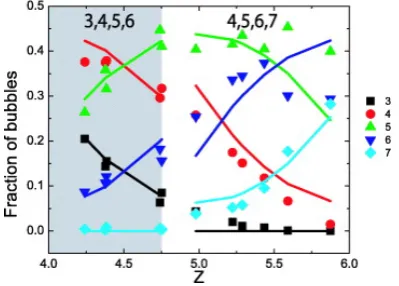
2.2.4 Distribution of Coordination Number

I now turn to the distribution of coordination numbers and present an empir-ical procedure, inspired in part by the analysis of van Hecke [21], reproduced in Figure 2.5 and Equations (2.5)-(2.8). The variance of van Hecke's data, σ2_{, was 0.75. Equations (2.5)-(2.8) were applied separately to the left and}

right parts of Figure 2.5.

Figure 2.5: Figure reproduced from [21] showing fractions of bubbles in the foam with n contacts as a function of Z. Solid lines: solutions to Equations (2.5)-(2.8) for the species listed at the top of the graph.

xn =

1 4

(Z₋(n+ 2))2+σ2₋1 2

(2.5)

xn+1 =

1 4

−(Z₋(n+ 1))2₋σ2+5 2

(2.6)

xn+2 =

1 4

−(Z₋(n+ 2))2₋σ2+5 2

(2.7)

xn+3 =

1 4

(Z₋(n+ 1))2+σ2₋1 2

[image:60.595.219.419.291.434.2]

(2.8)

(61)

4.0 4.5 5.0 5.5 6.0 Average Coordination Number, Z

0.0 0.1 0.2 0.3 0.4 0.5 0.6 0.7

F raction of bubbles with n neigh b ours 0 3 4 5 6 7 8 9 Plat Data Wet Dry

4.0 4.5 5.0 5.5 6.0

Contact number

Z

0.0 0.1 0.2 0.3 0.4 0.5 0.6 0.7

F

raction

of

bubbles

with

n

neigh

b

ours

n= 0

n= 3

n= 4

n= 5

n= 6

n= 7

n= 8

Soft Disk Data

[image:61.595.143.415.140.617.2]

Wet Dry

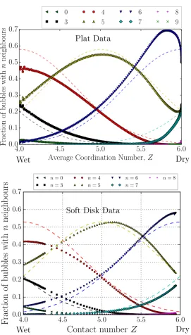
Figure 2.6: The fraction of bubbles with n neighbours as a function of average

coordination number, Z (top: Plat, bottom: Soft Disk). Simulation data

(sym-bols) can be approximated by the functional form of Equation (2.9) (dashed lines), with only a single t parameter σ'0.684±0.004for all the data. Note

(62)

of the distribution), as an adequate description of the data,

f(n) = 1 σ√2πexp

−(Z₋n)2

2σ2

, (2.9)

where Z is the coordination number, as above, and the value of σ used in Figure 2.6 is 0.684, which was found by a least squares t to the data. This can be considered to be a continuous analogue of Equations (2.5)-(2.8). It appears likely that the width of this distribution is connected with the polydispersity of the sample, but this has not been investigated yet. Note that in this analysis bubbles with 0, 1, and 2 neighbours are grouped together as having 0 contacts as they are all rattlers.

5

6

8

6

5

7

Figure 2.7: Example of a T1 transition where the average coordination number,

Z, is unchanged, but the distribution f(n) does change. The numbers indicate

the number of neighbours of each bubble involved in the T1.

(63)

0.00 0.02 0.04 0.06 0.08 0.10 0.12 0.14 0.16 Average Liquid Fraction φ

0.0 0.1 0.2 0.3 0.4 0.5 0.6 0.7

F

raction

of

bubbles

with

n

neigh

b

ours

0 3

4 5

6 7

[image:63.595.123.431.142.399.2]

8 9

Figure 2.8: The fraction of bubbles with n neighbours as a function of liquid

fraction, φ for the Plat simulations. Note the minimum in the fraction of ve

sided bubbles around φ _' 0.03 and the maximum in the fraction of six sided

bubbles around φ_'0.04.

(64)

0 0.1 0.2 0.3 0.4 0.5 0.6 0.7 0.8 0.9 1

0 0.02 0.04 0.06 0.08 0.1 0.12 0.14 0.16

Fraction of n -Sided Plateau Borders

Average Liquid Fractionφ

3 4 5 6 7 8 9 10 11

10

−8

10

−7

10

−6

10

−5

10

−4

10

−3

10

−2

10

−1

10

0

0 .

02 0

.

04 0

.

06 0

.

08 0

.

1 0

.

12 0

.

14 0

.

16 Fraction

of

n

-Sided

Plateau

Borders

Average Liquid Fraction

φ

[image:64.595.127.510.144.648.2]

3

4

5

6

7

8

9

10

11

Figure 2.9: Distribution of number of sides of Plateau borders as a function of liquid fraction. Top: The three sided Plateau borders clearly dominate the statistics for any φ.0.14. Bottom: The same data with a logarithmic y axis.

(65)

3.5 4 4.5 5 5.5 6

2

I

/

(

I

−

2)

[image:65.595.125.420.149.359.2]

Z

Figure 2.10: Euler's equation versus average coordination number [15]. I is the

average number of sides of the Plateau borders. The perfectly straight line veries that Euler's equation (Equation (2.10)) holds in the Plat simulations.

2.2.5 Distribution of Plateau Border Sides

For completeness, the distribution of the number of sides of the Plateau borders as a function of φ is shown in Figure 2.9. This data complements data presented by Hutzler and Weaire [15]. The previous dataset was very limited, while Figure 2.9 is very thorough and complete.

The distribution of number of sides of Plateau borders can be related to the average coordination number via Euler's equation

Z = 2I

I ₋2, (2.10)

(66)

2.3 Statistics of Bubble Rearrangements

As introduced in Section 1.2.5, the shear modulus and yield stress of foams go to zero in the wet limit. Hutzler et al. [36] observed an associated phenomenon, which can be considered to be an additional aspect of the critical behaviour associated with the wet limit. This is the occurrence of cascades of contact changes during equilibration in response to a small stress increment above the yield stress.

The size of the cascades was found to increase with the liquid fraction, possibly tending to innity (and thus preventing Plat from converging) at the wet limit. However, it was not feasible for Hutzler et al. to fully explore the wet limit, at which point the size of the cascades was expected to diverge. Here we return to this phenomenon, using a progressive increase of liquid fraction, rather than stress, as the small perturbation. Where the previous results had to rely on counting the number of contact changes that occurred over the course of the equilibration routine, we will use the technique of successive adjacency matrices described in Section 1.4.1 to approach this more thoroughly.

There are two types of elementary rearrangements in a two dimensional foam of nite liquid fraction, in which a contact between two bubbles is either gained or lost, see Figure 2.11. In what follows, I will count the fraction of bubbles involved in rearrangements in any given step, rather than the rearrangements themselves. Another alternative would be to measure changes in the energy of the system, as Durian did for the more rudimentary bubble model [34, 57] discussed in Section 1.4.2.

As the wet limit is approached, it becomes particularly evident that more elementary rearrangements are provoked by a small increment ofφ.

(67)

[image:67.595.82.473.180.477.2]

Dry Wet

Figure 2.11: Two alternative illustrations of rearrangements due to a small in-crease in liquid fraction. Top row − Red bubbles lose contacts, blue bubbles

gain contacts, and gray bubbles both gain and lose contacts. Bottom row −

Red is the liquid before rearrangements, blue is the liquid after rearrangements, and black is unchanged liquid. Left: in a dry foam (φ = 0.006), an increase

in liquid fraction ∆φ = 0.001 only leads to localised rearrangements. Centre:

example of extensive rearrangements in a moderately wet foam (φ = 0.112).

Right: Rearrangements involving nearly two thirds of all bubbles in a foam (φ= 0.149) close to the critical liquid fraction. Note that the regions in which

Models of wet two dimensional foams