Scholarship@Western
Scholarship@Western
Electronic Thesis and Dissertation Repository
4-22-2015 12:00 AM
Advanced Compression and Latency Reduction Techniques Over
Advanced Compression and Latency Reduction Techniques Over
Data Networks
Data Networks
Fuad Shamieh
The University of Western Ontario
Supervisor Dr. Xianbin Wang
The University of Western Ontario
Graduate Program in Electrical and Computer Engineering
A thesis submitted in partial fulfillment of the requirements for the degree in Master of Engineering Science
© Fuad Shamieh 2015
Follow this and additional works at: https://ir.lib.uwo.ca/etd
Part of the Digital Communications and Networking Commons
Recommended Citation Recommended Citation
Shamieh, Fuad, "Advanced Compression and Latency Reduction Techniques Over Data Networks" (2015). Electronic Thesis and Dissertation Repository. 2844.
https://ir.lib.uwo.ca/etd/2844
This Dissertation/Thesis is brought to you for free and open access by Scholarship@Western. It has been accepted for inclusion in Electronic Thesis and Dissertation Repository by an authorized administrator of
ADVANCED COMPRESSION AND LATENCY REDUCTION
TECHNIQUES OVER DATA NETWORKS
(Thesis format: Monograph)
by
Fuad Shamieh
Graduate Program in Electrical and Computer Engineering
A thesis submitted in partial fulfillment
of the requirements for the degree of
Masters of Engineering Science
The School of Graduate and Postdoctoral Studies
The University of Western Ontario
London, Ontario, Canada
c
Applications and services operating over Internet protocol (IP) networks often suffer from high latency and packet loss rates. These problems are attributed to data congestion resulting
from the lack of network resources available to support the demand. The usage of IP networks
is not only increasing, but very dynamic as well.
In order to alleviate the above-mentioned problems and to maintain a reasonable Quality of
Service (QoS) for the end users, two novel adaptive compression techniques are proposed to
reduce packets’ payload size. The proposed schemes exploit lossless compression algorithms
to perform the compression process on the packets’ payloads and thus decrease the overall
net-work congestion. The first adaptive compression scheme utilizes two key netnet-work performance
indicators as design metrics. These metrics include the varying round-trip time (RTT) and the
number of dropped packets. The second compression scheme uses other network information
such as the incoming packet rate, intermediate nodes processing rate, average packet waiting
time within a queue of an intermediate node, and time required to perform the compression
process.
The performances of the proposed algorithms are evaluated through Network Simulator 3
(NS3). The simulation results show an improvement in network conditions, such as the number
of dropped packets, network latency, and throughput.
Keywords: Compression, Congestion, TCP, UDP, Latency
Acknowledgments
First and foremost, I would like thank my supervisor, Dr. Xianbin Wang, for his continuous support, guidance, patience, and motivation. He encouraged me to pursue a deeper understand-ing of my areas of interest.
In addition to my supervisor, I would like to thank Dr. Ahmed Refaey, Dr. Auon Akhtar, and Dr. Hao Li for their continuous guidance and support.
My sincere appreciation and gratitude also goes to Steven Andrews, Kyle Doerr, and Mo-hamad Khalil for helping me throughout my thesis.
I would like to thank my friends Ali Al-Saady, Alfred Kenny, Antoan Antun, Rakan Duqum, and Scott Van Heesch for keeping my spirits up.
Last but not least, I would like to thank my parents, Jamal Shamieh and Naila Farraj, and my sister, Ilein Shamieh, for their endless support and encouragement.
Finally, I would also like to acknowledge the Faculty of Engineering, especially the Depart-ment of Electrical and Computer Engineering at Western University for the excellent facilities, libraries, and resources available to graduate students.
Abstract ii
Acknowledgments iii
Table of Contents iv
List of Figures vii
List of Tables ix
Abbreviations x
1 Introduction 1
1.1 Defining Networks . . . 2
1.2 Motivation - Network Congestion . . . 3
1.3 Proposed Solutions . . . 4
1.3.1 Adaptive Compression and Decompression Scheme Based on Real-Time Network Feedback . . . 5
1.3.2 Adaptive Distributed Compression and Decompression Scheme Utiliz-ing Intermediate Network Nodes . . . 5
1.4 Thesis Organization and Contribution . . . 5
2 Background Study on the Internet Protocol Stack, Network Delays, Compres-sion Algorithms, and Modes of CompresCompres-sion 8 2.1 Internet Protocol Stack Model Overview . . . 9
2.2 Internet Protocol Stack Layer Usage . . . 9
2.3 Application Layer . . . 11
2.4 Transport Layer . . . 12
2.4.1 TCP Operation . . . 12
2.4.2 UDP Operation . . . 16
2.4.3 TCP and UDP Checksum . . . 16
2.5 Network Layer . . . 17
2.6 Data-Link Layer . . . 19
2.7 Physical Layer . . . 20
2.8 Network Delays . . . 20
2.9 Compression Algorithms . . . 23
2.9.1 Lempel-Ziv Compression Algorithm . . . 24
LZ77 . . . 24
2.9.2 ZLIB . . . 27
2.10 Modes of Compression . . . 30
2.10.1 Stateless Compression . . . 30
2.10.2 Streaming Compression . . . 31
2.10.3 Offline Compression . . . 31
2.10.4 Block Compression . . . 32
2.11 Minimum Size for Performing Compression . . . 32
3 Literature Review on Compression Based Network Congestion Mitigation So-lutions 33 3.1 Introduction . . . 33
3.2 Compressing Packets Adaptively Inside the Network . . . 33
3.3 Adaptive On-the-Fly Compression . . . 35
3.4 IPzip: A Stream-Aware IP Compression Algorithm . . . 37
3.5 Delayed-Dictionary Compression for Packet Networks . . . 39
3.6 Adaptive Online Data Compression . . . 40
3.7 IP Payload Compression Protocol - IPComp . . . 41
3.8 Summary . . . 43
4 An Adaptive Compression Technique Based on Real-Time Network Feedback 45 4.1 Introduction . . . 45
4.2 Compressed and Non-compressed Packet Identification . . . 47
4.3 Flow of Operations . . . 48
4.3.1 Passive Mode . . . 48
4.3.2 Intermediate Mode . . . 51
4.3.3 Active Mode . . . 53
4.4 Implementation . . . 55
4.4.1 Software Implementation . . . 55
4.4.2 Hardware Implementation . . . 57
4.4.3 End-hosts Mutual Agreement and Mode Selection . . . 57
4.4.4 Compression Scheme Selection . . . 61
4.5 Simulation Model . . . 62
4.5.1 Performance Metrics and Results . . . 63
4.5.2 Analysis . . . 68
4.6 Summary . . . 72
5 Adaptive Distributed Compression and Decompression Scheme Utilizing Inter-mediate Network Nodes 74 5.1 Introduction . . . 74
5.2 Queueing Model for the Network . . . 76
5.3 Packet Generation Rate . . . 77
5.4 Compressed and Non-compressed Packet Identification . . . 80
5.5 Implementation . . . 80
Switching Fabric . . . 83
Output Ports . . . 83
Routing Processor . . . 84
5.5.2 Hardware Implementation . . . 85
5.5.3 Anatomy of An Advanced Intermediate Node/Advanced L3 Router . . 85
Software and Hardware Planes . . . 85
Input Ports . . . 87
Switching Fabric . . . 88
Output Ports . . . 88
Routing Processor . . . 89
5.5.4 Heuristic Algorithm . . . 90
5.6 Simulation Model . . . 92
5.7 Performance Metrics and Results . . . 93
5.8 Analysis . . . 97
5.9 Summary . . . 100
6 Conclusion 101 6.1 Conclusion . . . 101
6.2 Future Work . . . 106
6.2.1 First Set of Additions . . . 106
6.2.2 Second Set of Additions . . . 107
6.2.3 Simulation and Implementation . . . 107
Bibliography 109
Curriculum Vitae 112
List of Figures
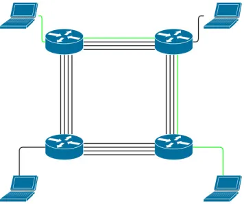
1.1 A Simple Circuit-Switched Network with Four Links and Four Routers . . . 2
1.2 A Simple Packet-Switched Network Suffering from Congestion . . . 4
2.1 Vertical Representation on the Usage of the Internet Protocol Stack . . . 10
2.2 The Internet Protocol Stack Layers Reference Model . . . 10
2.3 Application Layer Message Formulation by Header Encapsulation of Data . . . 12
2.4 TCP Three-Way Handshake Process . . . 13
2.5 TCP Header Structure . . . 14
2.6 Transport Layer Segment Formulation by Header Encapsulation of Upper Layer’s Data . . . 16
2.7 UDP Layer Header Structure . . . 16
2.8 Network Layer Datagram Formulation by Header Encapsulation of Upper Lay-ers’ Data . . . 17
2.9 IPv4 - Network Layer Header Structure . . . 18
2.10 Data-Link Layer Frame Formulation by Header and Trailer Encapsulation of Upper Layers’ Data . . . 19
2.11 Data-Link Layer Frame Structure . . . 19
2.12 Physical Layer Encoding and Transmitting Data in the Form of Bits . . . 20
2.13 LZ77 Sample of a Window and Lookahead Buffer Separated by a Coding Po-sition Indicator . . . 25
2.14 Simple Prefix Coding of Four Symbols . . . 28
3.1 Parking Lot Topology . . . 35
3.2 DDC Combined with LZ77 with a Delay ofδUnits . . . 40
3.3 IPComp Header Structure . . . 42
4.1 Network where the Compression and Decompression of Payloads Occurs Within the End-hosts. . . 46
4.2 Decision Tree to Identify a Packet’s Compression Status . . . 47
4.3 Passive Mode’s Logic and Method of Operation Flow Chart. . . 49
4.4 Intermediate Mode’s Logic and Method of Operation Flow Chart. . . 52
4.5 Active Mode’s Logic and Method of Operation Flow Chart. . . 54
4.6 The Location where the Implemented Scheme will Intercept Communications to Perform the Compression or Decompression Process . . . 55
4.7 A) Is the Packet Structure of a Regular Packet In a System Without Any Com-pression Scheme. B) Is the Packet Structure After Performing the ComCom-pression Operation. . . 56
4.9 ACK Packet Structure . . . 58
4.10 Routine Followed By End-hosts While Using the Compression Enabled Protocol 60 4.11 Passive Mode Simulation Results . . . 66
4.12 Intermediate Mode Simulation Results . . . 67
4.13 Active Mode Simulation Results . . . 67
5.1 Sample Network where the Compression and Decompression Processes Occur Within the Intermediate Nodes of the Network. . . 75
5.2 Parking Lot Topology With Intermediate Nodes Capable of Advanced Data Processing . . . 76
5.3 Queue View From the Intermediate Nodes’ Perspective . . . 76
5.4 Average Number of Packets in a Queue of an Intermediate Node as a Function ofρ . . . 79
5.5 Identifying if the Payload is Compressed or Otherwise . . . 80
5.6 Abstract View of L3 Router Architecture . . . 82
5.7 Input Port Stages Experienced by Packets . . . 83
5.8 Output Port Stages Experienced by Packets . . . 84
5.9 Advanced L3 Router Architecture . . . 86
5.10 Input Ports With Advanced Functionality and Three Distinct Queues . . . 87
5.11 Output Ports With Advanced Functionality to Perform the Required Compres-sion and DecompresCompres-sion Processes . . . 89
5.12 Simplified Algorithm for the Proposed Scheme . . . 91
5.13 Network Topology Used for the Simulation . . . 92
5.14 Simulation Results in the Absence and Presence of the Compression Scheme Under Different Network Loads . . . 97
List of Tables
2.1 Sample Latency Values for Different Networks of Various Speeds and
Dis-tances. The Size of Each Packet is 1500 bytes. . . 23
2.2 LZ77 Example - Sample Input String . . . 26
2.3 Encoding Process of the Input String Resulting in An Output of Tokens Indi-cating Matches Within the Original String . . . 26
2.4 Decoding Process where the Output of the Encoder is Treated as an Input . . . 27
2.5 An Example of Rearranging the Codes of Symbols . . . 29
3.1 CPI Values and Their Representation . . . 43
4.1 Sample EtherType Values . . . 48
4.2 Internal Network Values for Passive Mode . . . 64
4.3 Calculated Network Values for Passive Mode . . . 65
4.4 Internal Network Values for Intermediate Node . . . 65
4.5 Calculated Network Values for Intermediate Mode . . . 65
4.6 Internal Network Values for Active Mode . . . 65
4.7 Calculated Network Values for Active Mode . . . 66
5.1 Packet Generation Rate of Each Source Node as a Function of the Intermediate Node’s Forwarding Rate . . . 93
5.2 Simulation Results with the Source Node Generation Rate ofλ = 50% in the Absence of the Compression Scheme . . . 95
5.3 Simulation Results with the Source Node Generation Rate ofλ = 50% in the Presence of the Compression Scheme . . . 95
5.4 Simulation Results with the Source Node Generation Rate ofλ = 60% in the Absence of the Compression Scheme . . . 95
5.5 Simulation Results with the Source Node Generation Rate ofλ = 60% in the Presence of the Compression Scheme . . . 96
5.6 Simulation Results with the Source Node Generation Rate ofλ = 80% in the Absence of the Compression Scheme . . . 96
5.7 Simulation Results with the Source Node Generation Rate ofλ = 80% in the Presence of the Compression Scheme . . . 96
ACK Acknowledgment
API Application Programming Interface
BLRTT Baseline Round-Trip Time
CPI Coding Position Indicator
CSMA/CD Carrier Sense Multiple Access/Collision Detection
FCS Frame Check Sequence
FPGA Field Programmable Gate Array
HTTP HyperText Transfer Protocol
ICT Information and Communication Infrastructure
IP Internet Protocol
IPv4 Internet Protocol version 4
IPv6 Internet Protocol version 6
IRTT Instantaneous Round-Trip Time
LZ77 Lempel-Ziv
LZO Lempel-Ziv-Oberhumer
MSS Maximum Segment Size
MTU Maximum Transmission Unit
NBLRTT New Baseline Round-Trip Time
NS3 Network Simulator 3
P-K Pollaczek-Khinchin
P2P Peer-to-Peer
pps Packets Per Second
QoS Quality of Service
RTT Round-Trip Time
SDN Software Defined Networking
TCP Transmission Control Protocol
UDP User Datagram Protocol
VoIP Voice over Internet Protocol
WWW World Wide Web
Chapter 1
Introduction
The use of traditional, real-time, and delay sensitive applications and services over
in-formation and communications technology (ICT) infrastructure is becoming more popular.
Emerging real-time applications, such as data retrieval from data centers, are delay sensitive.
It follows that certain network performance metrics must be realized for an acceptable Quality
of Service (QoS). Maintaining these expectations is becoming more difficult because of the continuous increase in size and frequency of the generated and transmitted data.
The primary challenge to overcome is the instigated end-to-end delay as the behavior and
usage of a given network changes. The rapid growth of the number of clients and their dynamic
behavior within an Internet protocol (IP) network induces largely varying data flows, yielding
high data congestion. In order to improve the usage of real-time applications, end-to-end delays
must be reduced [1][2].
The particular focus of this thesis is the design and validation of different compression schemes that are adaptive in nature and easily deployed. The compression schemes attempt
to compress the payload of data packets being transmitted over a given network set-up. The
reduction in packet size after successfully applying compression results in an increase in
band-width utilization and a reduction in network congestion, thereby decreasing the number of
dropped packets.
The advantages of the compression schemes are enhanced bandwidth utilization and
in-creased number of active simultaneous network applications while maintaining a smooth
munication session. An adaptive compression scheme is preferable over a constant
compres-sion scheme for two reasons: the slight possibility of having a comprescompres-sion process that may
increase the overall transmission time, and increased number of CPU cycles [3][4].
In the following sections, a brief description of networks and the congestion problem is
given.
1.1
Defining Networks
Traditional communication networks operate over circuit-switched network configuration.
In circuit-switched networks, the route resources between a source-destination pair are reserved
over the transmission medium to guarantee a certain level of performance. The concept of
reserving network resources limits the number of simultaneous active source nodes as well
as the allocated bandwidth per node. Additionally, a certain amount of bandwidth must be
reserved at all times for a node whether it is active or not. To increase the number of nodes that
can transmit data over a network, as well as the bandwidth allocated per node, packet-switched
networks are deployed to replace circuit-switched networks. An example of a circuit-switched
network can be seen in Figure 1.11.
Figure 1.1: A Simple Circuit-Switched Network with Four Links and Four Routers
1.2. Motivation- NetworkCongestion 3
Packet-switched networks do not provide any service guarantees. These types of networks
are designed to allocate route resources for a source-destination pair on demand. Consequently,
packet switched networks are known as best-effort networks.
In such networks, messages generated by a source node are encapsulated into packets where
they experience the full link speed when transmitted. Nevertheless, a packet will experience
different types of delays throughout its journey, including transmission, propagation, queuing, and processing delay. An example of a packet-switched network can be seen in Figure 1.2.
The Internet is a complex example of a heavily used packet-switched network. The
de-vices connected to this network, such as end-hosts and routers, are physically and logically
connected together, as a result of which information can be exchanged. The exchanged
infor-mation includes data generated by real-time and traditional applications.
To successfully exchange data over packet switched networks, communication protocols
that exchange messages with certain commands and formats are used. Indeed, there is a
mul-titude of different protocols available for use to accomplish various tasks. A few examples of these protocols include congestion-control, routing data, and electronic mail protocol [5].
Today, societies rely on best-effort networks for different services although they are known for not providing any guarantees on packet delivery or QoS. Within such networks, it is
com-mon to have dropped packets, packets utilizing different routes between a source-destination pair, and congestion [9]. Due to the importance of these networks, it is necessary to improve
the condition of a communication session.
In this thesis, the focus will be on network congestion as described in the following section.
1.2
Motivation - Network Congestion
Congestion occurs when the incoming rate of packets exceeds the nodal processing rate.
As a result, packet loss as well as service degradation will occur. The reason behind the packet
packets may require retransmission and consequently the network latency may increase while
the QoS decreases. An example of network congestion can be seen in Figure 1.2.
Figure 1.2: A Simple Packet-Switched Network Suffering from Congestion
Precisely, the buffer of an intermediate node will be able to hold a finite number of packets, resulting in excess packets being dropped. Additionally, increasing the size of the memory of
an intermediate node will not solve the problem but rather will induce further congestion. The
increase in memory size will allow a larger queue of packets to form. The larger queue will
result in packets being queued for a longer period of time. If the packets are queued for long
enough to time out, a retransmission will be required [8]. Therefore the congestion problem
must be mitigated in a different manner.
The following section contains a brief introduction to the proposed solutions.
1.3
Proposed Solutions
To mitigate the congestion problem, two compression techniques are proposed. Both
tech-niques are designed to be adaptive to network conditions to ensure a higher performance. The
1.4. ThesisOrganization andContribution 5
1.3.1
Adaptive Compression and Decompression Scheme Based on
Real-Time Network Feedback
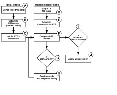
An adaptive compression scheme is proposed where the compression and decompression
processes occur within the end-hosts. In this scheme, the end-hosts determine whether to
enable or disable the compression process based on a certain network value known as
round-trip time (RTT). In simple terms, the RTT value is continuously observed and compared to
another value. Once the RTT value exceeds the other value by a certain threshold, the source
end-host will activate the compression scheme and commence the process of encoding data.
1.3.2
Adaptive Distributed Compression and Decompression Scheme
Uti-lizing Intermediate Network Nodes
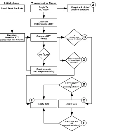
An adaptive compression scheme is proposed where the compression and decompression
processes take place within the intermediate nodes2 of the network. The intermediate nodes,
routing data from one node to another, are responsible for compressing packets’ payloads
ac-cording to the network condition. The network condition is determined by calculating certain
values, such as the average waiting time of a packet in the queue of an intermediate node,
based on certain queuing theory models. In this compression and decompression scheme, the
source-destination pairs are alleviated from the processes of encoding and decoding data.
1.4
Thesis Organization and Contribution
The main contribution of this thesis is the design and validation of the proposed
compres-sion schemes over networks utilizing the IEEE 802.3 standard for packet transmiscompres-sion in local
and wide area networks. The testing and validation process of the proposed schemes is
com-pleted using a popular open source simulation platform known as Network Simulator 3 (NS3).
2A router is a type of an intermediate node within a network. Any node within the network responsible for
There are many advantages of using NS3, such as allowing the user to rapidly implement and
prototype a network design as well as allowing the user to apply any necessary changes to the
platform.
The following points briefly outline the main contributions contained within:
• A novel compression and decompression scheme is proposed where it operates within the
end-hosts and employs lossless compression algorithms to maintain data integrity. Also,
the proposed scheme contains three different subschemes that are designed for different network types. Additionally, this scheme utilizes a multi-layer feedback value known as
the RTT to determine when to activate compression.
• A novel distributed compression and decompression scheme is proposed. The proposed
scheme operates by compressing and decompressing packets within the intermediate
nodes of a given network. Using queuing theory models and techniques, the intermediate
nodes within the network are capable of activating the compression and decompression
processes when necessary.
• The proposed schemes reduce network congestion. The reduced network congestion
yields lower end-to-end delays and number of packet drops as well as a smoother
com-munication session.
• The proposed schemes are seamless and transparent to the source-destination pairs as
they are designed to enhance communication sessions.
The remainder of the thesis is organized as follows:
• Chapter 2 provides a brief description of the Internet protocol stack, i.e., necessary
pro-tocols to initiate and complete transmission sessions on IP networks using the IEEE
1.4. ThesisOrganization andContribution 7
• Chapter 3 is the literature review of the other compression techniques available. A brief
summary of each existing and relative compression technique is given.
• Chapter 4 describes the design and validation of the RTT based compression technique.
Additionally, the algorithm for each of the subschemes is described and presented. Also,
the results and discussion of the conducted simulations for all of the sub-schemes are
included.
• Chapter 5 describes the design and validation of the distributed compression technique as
well as the queuing theory principles used. The results and discussion of the conducted
simulations under different network loads are included.
• Chapter 6 is the conclusion of the thesis and primarily consisting of the summary of the
Background Study on the Internet
Protocol Stack, Network Delays,
Compression Algorithms, and Modes of
Compression
An understanding of the Internet protocol stack and the different types of network delays is essential to mitigating congestion in data networks. Every packet traversing within a data
network experiences different types of delays as a result of using the Internet protocol stack as a model to achieve end-to-end communication. Although these delays can be minimized, they
are inevitable.
The types of delays are easily categorized as nodal and transmission delays. The network
delays are used to calculate important values, including the RTT and several buffer sizes of network devices. It is therefore important to utilize and understand the collected information
from the network delays.
In this chapter, an overview of the Internet protocol stack and the delays experienced by a
packet is given. The lossless compression algorithms used in this thesis are reviewed. Finally,
a brief discussion regarding the concept of the minimum acceptable size of packets is included.
2.1. InternetProtocolStackModelOverview 9
2.1
Internet Protocol Stack Model Overview
The Internet protocol stack is a multi-layered network architecture consisting of at least
5 layers, used to provide end-to-end connectivity between source-destination pairs. Each of
the 5 layers performs a set of well-defined services and functions to ensure the connectivity
between end-hosts. These services and functions include data formatting, addressing, routing,
and transmission, among others.
This communication model is hierarchical; the lower layers provide services for the higher
layers. When two end-devices are communicating with each other, the transferred data passes
through all of the layers. Depending on the application performing the transmission and the
re-quired service type, the relevant protocols are used to initiate and complete the communication
session.
For the source, data is generated by an application at the highest layer. The generated data is
passed down to the lower layers, where each layer adds a header. The headers contain sensitive
information, such as addresses, ports, and sequence numbers of the data being transmitted.
The lowest layer, i.e., the physical layer, is responsible for the transmission of the data. At the
destination, the received data moves upwards through the layers in order, where the headers
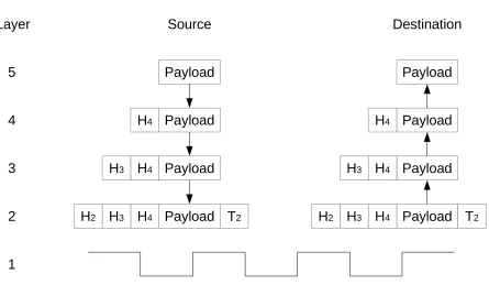
are removed as the data progresses [10]. An abstract representation of a functioning Internet
protocol stack can be seen in Figure 2.1.
2.2
Internet Protocol Stack Layer Usage
In any given network, communication devices must follow certain protocols to successfully
exchange messages. Different network entities and applications demand different types of pro-tocols for various reasons, including: QoS provisioning, congestion control, delay sensitivity,
etc. Combining all of the available protocols creates the protocol stack [5].
The Internet protocol stack, starting from top to bottom, consists of at least 5 layers:
Payload
Payload
Payload
Payload H4
H4
H4
H3
H4
H3
H2 T2
Payload
Payload
Payload
Payload H4
H4
H4
H3
H4
H3
H2 T2
Source Destination
5
4
3
2
1 Layer
Figure 2.1: Vertical Representation on the Usage of the Internet Protocol Stack
protocols for network entities to use. The Internet protocol stack can be seen in Figure 2.2.
Application Layer
Transport Layer
Network Layer
Data-Link Layer
Physical Layer
Figure 2.2: The Internet Protocol Stack Layers Reference Model
2.3. ApplicationLayer 11
different layers in order for the message to reach its destination. At various points throughout the network, such as routers and switches, some headers are stripped and new ones are attached
prior to the message reaching its destination. Each header of the different layers contains information about the message including: application, source address, destination address,
source port number, destination port number, payload size, etc. [5].
The following sections discuss the different layers of the Internet protocol stack in detail, starting with the uppermost layer.
2.3
Application Layer
Internet applications such as voice-over-Internet-protocol (VoIP), peer-to-peer (P2P) file
sharing, emails, World Wide Web (WWW), and multi-player online gaming are the motivating
force behind the expansion of the Internet. Internet applications are built to run on end-hosts;
the user therefore does not have to write any software for the routers and switches within the
network in order for the application data to reach its destination [11].
One of the main kinds of application architectures is known as client-server architecture.
In this architecture, a fixed, dedicated, and always available server with a static, known IP
address is responsible to service requests from clients. Additionally, clients do not directly
communicate with each other; the server is responsible for transferring data between the clients.
Moreover, such that they can respond to a large number of requests efficiently, servers are usually housed in large data centers [11].
The client and server exchange requests and messages over the network using sockets.
A socket is the application programming interference (API) between the application layer,
transport layer, and network. A socket allows hosts and processes to exchange messages over
a network by identifying each other using IP addresses and port numbers, respectively [11].
The structure of the exchanged messages between the client-server applications is defined
own header to the generated data. An example of an application layer protocol is HyperText
Transfer Protocol (HTTP), which is widely used by the WWW [11][12].
Application Layer App Layer Header Data
Figure 2.3: Application Layer Message Formulation by Header Encapsulation of Data
2.4
Transport Layer
Underneath the application layer lies the transport layer. The primary purpose of this layer
is to provide logical, efficient, end-to-end communication services between the application layer processes of different end-hosts [13]. To achieve end-to-end communication, the transport layer provides two main protocols.
Two distinct protocols with different properties are present in the transport layer and they are used for transferring segments of data. The first protocol is known as User Datagram
Protocol (UDP) and the second one is Transmission Control Protocol (TCP). It is known that
UDP is unreliable and connectionless whereas TCP is known to be connection oriented and
full duplex. Furthermore, UDP and TCP provide data integrity check by including a
pre-transmission error detection header field known as the checksum [14].
2.4.1
TCP Operation
The services provided by the TCP protocol include flow control, reliable data transfer,
transmission flow multiplexing, retransmission of packets, and security measures. The TCP
protocol pushes and forwards data when necessary while assuring the sending and receiving
parties that the transmitted data is not damaged, lost, duplicated, or delivered out of order.
To provide the aforementioned services, TCP uses a segment sequence numbering system as
well as an acknowledgement (ACK) mechanism where the receiving end ACKs the received
2.4. TransportLayer 13
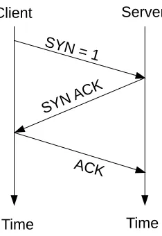
To initiate a TCP connection, a three-way handshake process takes place, as shown in
Figure 2.4. This is done by the client setting the SYN field in the TCP header to 1 and sending
the SYN segment to the server. Once the server receives the SYN segment, the server allocates
the receiving buffer and replies to the client with a SYNACK segment. Finally, the client allocates a receiving buffer and sends an ACK segment to the server. A similar process is used to terminate the connection, however the FIN field is used rather than the SYN field [15]. The
TCP header structure is shown in Figure 2.5.
Client Server
Time Time
SYN = 1
SYN AC
K
ACK
Figure 2.4: TCP Three-Way Handshake Process
While using TCP, the receiver organizes segments, ACKs data, and discards duplicates
according to the segments’ sequence numbers. Furthermore, the receiver uses a checksum
mechanism to identify damaged segments. Precisely, the receiver verifies the checksum field
in the TCP header by computing the checksum value [15].
The ACK messages are also used for flow control by informing the sending party of the
receiver’s buffer size. Along with the ACK message, the receiver’s buffer window size is returned to the sender whilst indicating the next acceptable packet sequence number [15]. This
is the receiver’s method of informing the sender which packet is expected.
The sequence number assigned to segments and their ACKs work together to provide
32 bits
8 bits 8 bits 8 bits 8 bits
Source Port Destination Port
Sequence Number Acknowledgement Number Header Length Field Unused Field U R G A C K P S H R S T S Y N F I N Window Size
Checksum Urgent Pointer
Options Field Upper Layer Data
Figure 2.5: TCP Header Structure
ACKing of segments. The sequence numbering field assigns numbers to the first byte in each
transmitted segment. For example, if the data size is 10,000 bytes whereas the maximum
seg-ment size (MSS) is 1000 bytes, the first segment is assigned a sequence number of 0, the second
segment is assigned a sequence number of 1000, and so on. The ACK field is defined by the
receiver and its value is set to be the sequence number of the next expected byte. For example,
if the receiving end-host received all bytes from 0 to 999, the receiver will set the ACK field to
1000 and send it back to the sending end-host. Using ACKs and sequence numbers, the sender
can identify which packet is lost or damaged and perform a retransmission if necessary [16].
When data is transmitted over a network using TCP, the receiver has a buffer window where the application will read the data from. The application does not necessarily read the data in
the buffer instantaneously. However, to prevent the possibility of overflowing the buffer, TCP provides a flow-control service where the speed of the application reading the buffer is matched to the speed of the data being received. This is accomplished by having the sender maintain a
2.4. TransportLayer 15
rwnd =RcvdBS −[LBRead−LBRcvd], (2.1) whererwndis the receive window size, RcvdBS is the allocated receiving buffer size, LBRead is the number of the last byte read by the application in the buffer, and LBRcvd is the number of the last byte received by the buffer.
On the other side of the flow, the receiver keeps track of the last byte sent and the last byte
ACKed. By keeping the difference of these two variables less thanrwnd, the sender will not overflow the receiver’s buffer [16]. The relationship of the variables is defined by equation (2.2):
LBS ent−LBACKed≤rwnd. (2.2)
Along with keeping track of therwnd size, the sender keeps track of another variable that
defines the congestion widow size, also known as cwnd. The cwnd value is defined by the
sender as the perceived network congestion where network congestion refers to the buffers of the intermediate nodes, such as routers and switches. The value of the cwnd affects the protocol’s transmission rate, that is whether the sender should increase or decrease the rate
[16]. Equation (2.3) defines the allowed amount of unacknowledged data with respect to the
size ofcwndandrwnd.
LBS ent−LBACKed≤min{cwnd,rwnd} (2.3)
In order for the TCP protocol to accomplish the aforementioned services, a header is
at-tached to the upper layer data and the packet will be referred to as a segment, as shown in
Transport Layer HeaderTCP Upper Layer'sData Segment
Figure 2.6: Transport Layer Segment Formulation by Header Encapsulation of Upper Layer’s Data
2.4.2
UDP Operation
The UDP protocol is a much simpler protocol when compared to TCP. It is a connectionless
protocol with a very small overhead. It does not provide any congestion control, ACKing
methods, sequence numbering, or retransmissions and it assumes that the IP provided by the
networking layer is used.
32 bits
16 bits 16 bits
Source Port Destination Port
Length Checksum
Upper Layer Data
Figure 2.7: UDP Layer Header Structure
2.4.3
TCP and UDP Checksum
Both TCP and UDP have an error detection mechanism known as verifying the checksum.
The checksum field holds a 16-bit value and is used to detect errors such as any changes to
the header segment as the segment moves from the source to the destination. The value of the
checksum is calculated at the sender by adding all 16-bit words in the UDP or TCP header, such
as the source and destination port numbers, followed by calculating the sum’s 1s complement.
Therefore, the 1s complement will be the value in the checksum field. On the receiving end,
the receiver will verify the checksum by adding all of the 16-bit words in the header as well
2.5. NetworkLayer 17
1111111111111111.
2.5
Network Layer
The application and transport layers rely on the forwarding and routing services of the
network layer to provide communication means between hosts. The forwarding function is
used by routers to direct incoming packets on to the appropriate output path using forwarding
tables. A routing function is used to determine the path taken by packets while traversing
between a source-destination pair [17].
The network layer provides the IP protocol as service for the upper layers. When an upper
layer segment is encapsulated with IP version 4 (IPv4) header, it is known as an IPv4 datagram
[18]. Figure 2.8 shows the network layer encapsulation of data passed from the transport layer.
Network Layer HeaderIP Uppler Layers'Data Datagram
Figure 2.8: Network Layer Datagram Formulation by Header Encapsulation of Upper Layers’ Data
The contents of the IPv4 header are shown in Figure 2.9. It can be seen in the IP header
that there are some important fields directly related to the size of the data. These fields are:
total length, datagram fragmentation related fields, and header checksum.
The total length field is a 16-bit field that includes the entire datagram length. The header
length field is specific to the size of the IP header [17]. According to equation (2.4):
T otalLength−HeaderLength= Data, (2.4) where subtracting the header length field from the total length returns the data size. Since the
32 Bits
8 Bits 8 bits 8 Bits 8 Bis
Version Header
Length Type of Service Total Length
Indetifier D
F M
F
Fragment Offset
Time-To-Live Protocol Header Checksum
Source Address Destination Adress
Options Upper Layers' Data
Figure 2.9: IPv4 - Network Layer Header Structure
The fragmentation related fields are: identifier, flag fields, and fragment offset. The data-gram is fragmented because the data-link layer frames have a maximum transmission unit
(MTU) of 1500 bytes. Therefore, large payloads must be fragmented and identified using
the 16-bit identifier field. The sender increments the value of the field with every transmitted
packet. Furthermore the receiver uses the identifier, flag, and fragment offset fields to reassem-ble datagrams [18].
There are two 3-bit flag fields available for use. From Figure 2.9, the DF and MF fields
are known asdo not f ragment andmore f ragments, respectively. If the DF field bits are set
to 0, it indicates that the datagram is not fragmented. If the packet cannot be fragmented, the
intermediate routers will discard it where a reply message is sent to the sender stating that
fragmentation is needed. If the MF field bits are set to 1, it indicates that more fragments are
expected. The receiver expects to receive packet fragments until the MF field bits are set to 0
[18].
2.6. Data-LinkLayer 19
2.6
Data-Link Layer
The primary purpose of the data-link layer is to frame datagrams received from the network
layer by adding a header and a trailer. The data-link layer is also used to establish a virtual link
for the network layer of the source end-host to the network layer of the destination end-host.
When a datagram reaches the data-link layer from the network layer, the datagram is framed
by concatenating a header to the beginning of the datagram as well as a trailer to the end of the
datagram, thus forming a frame. The newly formed frame is now transmitted over a physical
medium via the physical layer [19] [20].
Data-Link Layer MAC/LLC Header Upper Layers'Data FCS Frame
Figure 2.10: Data-Link Layer Frame Formulation by Header and Trailer Encapsulation of Upper Layers’ Data
8 Bytes 6 Bytes 6 Bytes 2 Bytes 46 to 1500 Bytes 4 Bytes
Preamble Dest. Address Src. Address EtherType Data FCS
Figure 2.11: Data-Link Layer Frame Structure
The data field in Figure 2.11 contains the datagram from the layer above where the MTU is
1500 bytes. Therefore, if the data size is greater than 1500 bytes, the data is fragmented.
Fur-thermore if the data is less than 64 bytes, the data is padded with zeros [19]. The encapsulated
data in the data field is checked for errors by a receiver using the frame check sequence (FCS)
2.7
Physical Layer
The final layer in the Internet protocol stack is the physical layer. It is responsible for
physically moving transmitted data, bit-by-bit, across a link, from a network device to another.
This is achieved by varying the voltage or current across the transmission medium.
There are network devices that only use the physical layer, such as repeaters and hubs. The
job of such low-layer devices is to accept incoming bits and forward them to the right output
[22] [23].
Physical Layer 01010101110101 Bits
Figure 2.12: Physical Layer Encoding and Transmitting Data in the Form of Bits
2.8
Network Delays
In any packet-switched network, all of the transmitted packets suffer from primarily four types of delays including: nodal processing delay, queuing delay, transmission delay, and
prop-agation delay. These delays are inevitable, and each packet experiences all of these delays at
every node along its journey from a source to a destination. Such delays are summed together
and referred to as the total nodal delay.
• Nodal Processing Delay:
As previously mentioned, every packet has a header and a payload that are attached
together and transmitted as a whole. For an intermediate node, such as a router or a
switch, to determine the path the packet will take, the node must process and examine
the packet’s header. In certain situations, other processing takes place, such as error
checks. The time needed to examine and process the packet is known as the processing
2.8. NetworkDelays 21
• Queuing Delay:
Intermediate nodes have the capability of buffering packets in case the network is con-gested. If a packet is queued, the time the packet waits until it is placed on the link is
known as the queuing delay. The time that the packet waits in the queue depends on the
number of packets that are located within the queue. If the queue is empty, the queuing
delay will be minimal, however, if the queue has a substantial number of packets, the
queuing delay will be large [5].
• Transmission Delay:
Transmission delay is time needed to transmit or push a packet into a link. This type of
delay is directly proportional to the size of the packet as well as the speed of the link.
The delay is defined according to equation (2.5).
Ttrans =
L
R, (2.5)
whereLis the size of the packet in bits andRis the transmission speed of the link from
one node to another [5].
• Propagation Delay:
Propagation delay is defined by the physical distance a bit must travel from one node to
another. Depending on the medium used to transmit the data, such as fiber optics cable
or twisted pair copper wire, the propagation speed will differ. The propagation speed will range from approximately 2∗108to 3∗108meters per second. The propagation delay is
defined according to equation (2.6).
Tprop =d/s, (2.6)
• Nodal Delay:
Thus, the total delay for a packet traveling from one node to another is defined according
to the following equation:
Tnodal=Tproc+Tqueue+Ttrans+Tprop, (2.7)
whereTproc andTqueueare usually neglected due to their minute effect on the total delay
[5].
• Round-Trip Time (RTT):
RTT is the total time needed for a packet to travel from a source node to a destination
node and back to the source node [6]. However in this thesis, the definition of RTT will
be slightly changed to the total time needed for a packet to travel from a source node to
a destination node in addition to the length of time needed for an ACK to travel from the
destination node to the source node.
• Latency:
Latency is the length of time it takes a packet to travel from the source to the destination
node [7]. Table 2.1 contains sample latency values for a 1500 bytes packet. The queuing
and processing delays are ignored due to their minute effect on the total time. The prop-agation speed considered was 2/3∗3∗108 = 2∗108 m/s. To calculate the latency for
the different scenarios, the following equation was used:
2.9. CompressionAlgorithms 23
Distance Propagation Delay Link Speed Transmission Delay Latency
1 km 5µs
1 Mbps 12 ms 12.005 ms
10 Mbps 1.2 ms 1.205 ms
100 Mbps 0.12 ms 0.125 ms
10 km 50µs
1 Mbps 12 ms 12.05 ms
10 Mbps 1.2 ms 1.25 ms
100 Mbps 0.12 ms 0.17 ms
100 km 500µs
1 Mbps 12 ms 12.5 ms
10 Mbps 1.2 ms 1.7 ms
100 Mbps 0.12 ms 0.62 ms
Table 2.1: Sample Latency Values for Different Networks of Various Speeds and Distances. The Size of Each Packet is 1500 bytes.
2.9
Compression Algorithms
There are two primary types of data compression, particularly, lossless and lossy
algo-rithms. In lossy compression, it is acceptable to have an encoded output file that is slightly
different than the input. Furthermore, lossy compression algorithms are primarily used with audio and video files where the quality of the image or video is directly affected by the com-pression level. Usually, higher quality images have a lower comcom-pression level.
In lossless compression, the purpose of the algorithm is to reduce the number of bits
re-quired to represent information through different means of encoding and decoding. Further-more, lossless compression guarantees the integrity of the original information, thus when the
encoded data is decoded, the decoded data is an exact replica of the original data [24].
In this work, all of the algorithms used are lossless compression algorithms. The
com-pression algorithms used are Lempel-Ziv-Oberhumer (LZO) and ZLIB. LZO is a lossless
compression algorithm based upon the original Lempel-Ziv (LZ77) compression algorithm.
LZO is also known to be an algorithm that favors speed over compression ratio whereas ZLIB
prefers compression ratio over speed [25]. Moreover, compression ratio is defined according
C = CDS
UCDS, (2.9)
whereCDS is the compressed data size andUCDS is the uncompressed data size [26].
The following subsections provide a brief overview of each algorithm.
2.9.1
Lempel-Ziv Compression Algorithm
Lempel-Ziv is a universal lossless compression algorithm developed in 1977 by Abraham
Lempel and Jacob Ziv. This algorithm does not rely on any prior knowledge of the source
statistics and depends on a learning process for discrete source characteristics [27].
LZ77
The LZ77 is a lossless dictionary-based compression algorithm that utilizes the longest
matching string concept and a sliding window approach to encode data [25]. The algorithm
treats an input string of bytes as two main parts where the large part consists of decoded data
and the smaller part consists of a lookahead buffer.
The decoded data is used as a dictionary for the lookahead buffer, where the algorithm looks for matches between the two parts. Once matches are found, output tokens are created
pointing to the location, length, and the first character seen in the lookahead buffer [24]. In other words, the algorithm reads and analyses a string of data where redundant information is
replaced by tokens containing information on how to retrieve the original information from the
encoded data.
There are important terms one must know to understand how compression works. These
terms include: input string, coding position indicator (CPI), lookahead buffer, window, and output. The following is the list of the terms with their respective definitions.
• Input string:
2.9. CompressionAlgorithms 25
...ABABABAAAA AAAA....
Input String Lookahead Buffer Coding Position
Figure 2.13: LZ77 Sample of a Window and Lookahead Buffer Separated by a Coding Position Indicator
• CPI:
CPI is the point where the lookahead buffer begins. The coding position indicator can be seen in Figure 2.13.
• Lookahead buffer:
The lookahead buffer contains bytes from the input data located after the CPI.
• Window:
The size of the window is used to indicate the number of bytes considered prior to the
coding position indicator. The window is empty at the beginning of the compression
pro-cess. As the input string is processed, the window will grow in size until reaching a size
ofw. When the window is of sizew, the sliding window approach occurs. The window
will slide according to number of bits encoded from the lookahead buffer, placing the coding position indicator in a new location.
• Output:
The output of the encoding process is mainly a pointer in the format of (LB,L) with a
terminating characterC(c). The output is represented by (LB,L)C(c), however, it is not
necessary to always includeC(c).
TheLB term is a value indicating the number of bytes the decoder should go back in the
position indicated by LB. The terminating character C(c) indicates the first byte in the
lookahead buffer located after the match indicated by the pointer.
In the event of no matches being found between the lookahead buffer and the sliding window, the output is a null pointer concatenated withC(c).
The following is an example of encoding a string of data using LZ77 approach. The string
of data is shown in Table 2.2.
Position 1 2 3 4 5 6 7 8 9
Byte A A B C B B A B C
Table 2.2: LZ77 Example - Sample Input String
The encoding process begins by reading the input string of bytes from Table 2.2. The
coding position indicator is placed at the first location, position 1, and is continuously moved. If
there are no matches, the output will be a null pointer with the terminating character; however,
if a match is found, the output will be a pointer with the terminating character. Table 2.3 shows
the output of the encoding process.
Step Position Match Terminating Character Output
1 1 – A (0,0)C(A)
2 2 A – (1,1)
3 3 – B (0,0)C(B)
4 4 – C (0,0)C(C)
5 5 B – (2,1)
6 6 B – (1,1)
7 7 ABC – (5,3)
Table 2.3: Encoding Process of the Input String Resulting in An Output of Tokens Indicating Matches Within the Original String
The decoder processes the output of the encoder and appends the bytes together in order.
More precisely, the output pointer and terminating character of the encoding process are now
2.9. CompressionAlgorithms 27
2.4 shows the process of decoding data and how the output of Table 2.3 is used as an input to
retrieve the original string.
Step Input Append Bytes Output String
1 (0,0)C(A) A A
2 (1,1) A A A
3 (0,0)C(B) B A A B
4 (0,0)C(C) C A A B C
5 (2,1) B A A B C B
6 (1,1) B A A B C B B
7 (5,3) ABC A A B C B B A B C
Table 2.4: Decoding Process where the Output of the Encoder is Treated as an Input
As seen from Tables 2.3 and 2.4, an input string was encoded using the sliding window and
longest matching string approach. The output of the encoder was a series of pointers indicating
the matches, if any, and the terminating character. The decoder processed the output of the
encoder to retrieve the original string [28]. It can be seen that the retrieved string from Table
2.4 was an exact replica of the input string presented in Table 2.2.
2.9.2
ZLIB
The ZLIB compression algorithm is a lossless algorithm that uses the DEFLATE
com-pressed data format for compressing an input string of data. More precisely, the DEFLATE
algorithm utilizes a combination of the LZ77 algorithm and Huffman encoding [29], thusly achieving a high compression ratio, when compared to LZO [31]. Furthermore, the algorithm
functions by dividing the input string into blocks and processing each block separately. Having
the blocks processed separately results in each one having its own independent series of Huff -man trees. However, the LZ77 algorithm will search for matches between the current block
and previously encoded blocks.
The output of the compression algorithm consists of encoded blocks where each block has
about the encoded data as well as the actual encoded data. The encoded data has a similar
structure as that of LZ77, where pointers are used to indicate matching and non-matching
strings. To be precise, the pointers are in the format of (L,LB), where L is the length of the
match andLBis the backward distance the decoder has to move to locate the match. A Huffman
code tree is allocated to provide details about the unmatched strings as well as Lwhereas the
other tree is used to provide information aboutLB [29].
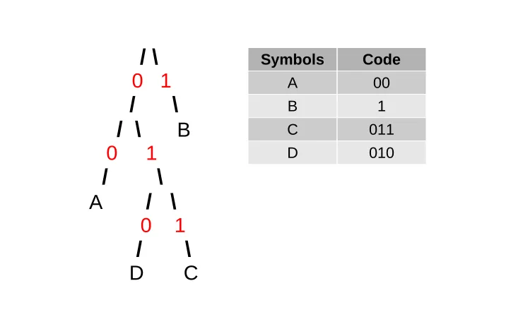
Prefix coding is used to assign each symbol from a given alphabet a sequence of bits to use
as means of representation. The sequence of bits, also known as codes, are unique per symbol
where the decoder may parse the the encoded symbols by analyzing the bits from the encoded
input. One may think of this procedure as shown in Figure 2.14 .
/ \
0 1
/ \
/ \
B
0 1
/ \
A
/ \
0 1
/ \
D C
Symbols Code
A 00
B 1
C 011
D 010
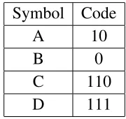
Figure 2.14: Simple Prefix Coding of Four Symbols
Huffman coding allows the construction of the optimal prefix code tree if the symbol fre-quency of a given alphabet is known. The optimal tree is constructed by allocating the shortest
codes for the symbols with the highest frequency of occurrence. Additionally, bit sequences
of the same length are in lexicographical order. Furthermore, shorter bit sequences
2.9. CompressionAlgorithms 29
as shown in Table 2.5. From Table 2.5, one can see that 110 and 111 are lexicographically
consecutive.
Symbol Code
A 10
B 0
C 110
D 111
Table 2.5: An Example of Rearranging the Codes of Symbols
Based on the lexicographical ordering rules, the Huffman codes for an alphabet are defined by using the lengths of the codes for each symbol, thus the lengths of the codes in Table 2.5 are
(2,1,3,3). Once the lengths of the codes are given to the Huffman algorithm, the algorithm will proceed by counting the number of codes of the same length. Subsequently, the algorithm will
compute the smallest numerical value for each code length. Finally, the algorithm will assign
consecutive numerical values for all the codes of the same length starting with the smallest
determined value from the previous step.
The following is an example of assigning codes to symbols.
• Assume an alphabet ABCDEFGH with bit lengths (3,3,3,3,3,2,4,4). The algorithm will
start by counting how many symbols are represented by a certain number of bits.
Number of Bits Count
2 1
3 5
4 2
• The algorithm will now calculate the lowest values of the given code lengths.
Number of Bits Lowest Value
2 0
3 2
Symbol Length Code
A 3 010
B 3 011
C 3 100
D 3 101
E 3 110
F 2 00
G 4 1110
• Finally, the algorithm will assign values to all the symbols.
After the construction of the Huffman trees, the encoded blocks containing the Huffman trees as well as the encoded data are formed. Each block has a 3-bit header specifying whether
the current block is the last block or not, as well as whether the block is compressed or not.
2.10
Modes of Compression
The ability to compress an input string using different approaches enables the user to achieve different levels of compression. There are primarily four different approaches to com-pressing a string of data. Each approach has certain advantages and disadvantages, however,
the proper approach must be used to achieve the desired results. The four approaches of
com-pression are: stateless, streaming, offline, and block compression.
2.10.1
Stateless Compression
The stateless compression approach is when packets are compressed and decompressed
independently, with absolutely no relationship to any other packet. Stateless compression is
also known as packet-by-packet compression where the receiver may perform a decompression
process on each packet independently. This approach of compression and decompression is
2.10. Modes ofCompression 31
2.10.2
Streaming Compression
The streaming compression approach, also known as continuous compression, is an
attrac-tive approach when reliable means of communication are available. Whilst using streaming
compression, packets are compressed and decompressed with a degree of interdependence.
Each packet is compressed using the history of the previously compressed packets as well as
the data within the current packet. Consequently, the receiver must decompress packets in
successive order [3].
Since the receiver must decompress packets in successive order, dropped packets will
in-duce a high latency 1 as the receiver waits for their arrival. Furthermore, the receiver must
have a rather large buffer, as it may need to store a hefty number of packets until all necessary packets arrive to perform the decompression process [3].
2.10.3
O
ffl
ine Compression
The offline compression approach is used when compression is performed at the end-hosts rather than the intermediate nodes of the network. This approach takes place at the higher
layers of the Internet protocol stack and is capable of achieving higher compression ratios
when compared to the other approaches.
In this approach, data is compressed as a complete unit, in blocks, rather than in small
chunks. Furthermore, the receiver is not required to store all of the packets in a buffer to per-form the decompression process; instead, the receiver will forward the packet to the higher
layers for further processing. Finally, it would be redundant for intermediate nodes to perform
any sort of compression on the packets’ payloads since the payloads are already compressed
[3].
2.10.4
Block Compression
The term block compression refers to a conglomerate of data being compressed at once.
A lossless compression algorithm with an excellent compression ratio is considered, such as
ZLIB, to better explain the difference between block and packet-by-packet compression. When using ZLIB as a compression algorithm, payload compression in blocks will provide a better
compression ratio due to the availability of a longer stream of data, which in turn provides
better matches of duplicate strings [30]. However, when transmitting the compressed data that
is originally compressed as a block, the receiver must wait for the entire stream of data to arrive
before processing it.
If the receiver holds on to data before processing it, two major problems arise. The first
problem is that the receiver must have a rather large buffer to store the received packets. The second problem is the possibility of dropped packets, which will result in a significant delay
[3]. This delay is broken down to processing, decompression, and transmission delays. The
dropped packets must be retransmitted or the received data will be rendered useless. Also
holding the packets in the buffer while waiting for a retransmitted packet may result in other packets being dropped due to a full buffer.
2.11
Minimum Size for Performing Compression
From [3], packets with a larger payload produce a better compression ratio since the
com-pression algorithm has a longer input string to find matches. To determine the minimum and
maximum size of a packet, one must consider two important aspects. The first aspect is the
collision detection mechanism where a minimum frame length is needed to determine whether
a collision occurred or not. The minimum frame length needed for collision detection depends
on the speed of the link as well as the length of the link. The second aspect is the desired
compression ratio where if a higher compression ratio is needed, the required size of packet
Chapter 3
Literature Review on Compression Based
Network Congestion Mitigation Solutions
3.1
Introduction
In this chapter, wide and local area network congestion control techniques via compression
are discussed. There is a variety of literature available on techniques that perform compression
within and outside the network. The following is a review of selected literature.
3.2
Compressing Packets Adaptively Inside the Network
In [26], the authors discussed mitigating induced traffic congestion over IP networks us-ing an adaptive lossless compression technique. This technique was deployed within a given
network rather than at the end-nodes to achieve greater compression efficiency and enhance the performance of the network as a whole. Moreover, the authors state that the
intermedi-ate relay nodes used to achieve compression within the network were capable of performing
advanced computational functions such as packet storage and processing as well as the
tradi-tional forwarding function. Furthermore, the authors state that in a non-congested network,
data compression may be redundant and there may be a slight risk of performance degradation
rather than enhancement.
To avoid the creation of a bottleneck situation within the network, the authors in [26]
pose three conditions designed to achieve an effective compression technique.
• All packets from all source nodes are compressed within the intermediate nodes unless
the packet has been compressed prior to arriving to the next intermediate node.
• If a packet is eligible for compression, it will only be compressed after meeting a certain
criteria.
• Packets are compressed individually, rather than in a block.
The criteria under which a packet is compressed is if an intermediate node receives a packet
with a regular sized payload, the intermediate node will calculate the waiting time of the packet
in the queue. If the waiting time is greater than a certain instantaneously calculated threshold,
the node will compress the packet’s payload.
W ≥C−(1−R)∗S/B, (3.1)
whereW is the waiting time of a packet within the relay queue of an intermediate node,C is
the time required to perform the compression process of a packet,S is the packet size, Bis the
bandwidth of the intermediate node’s output link, andRis the compression ratio.
If equation 3.1 and the aforementioned conditions are satisfied, the intermediate node will
compress the packet, otherwise it will not and it will forward the packet without additional
processing.
The proof of concept was conducted on the Network Simulator 2 (NS2) platform with
certain necessary and valid assumptions. Additionally, the network topology used was the
parking lot topology, as shown in Figure 3.1.
The simulation assumptions were:
• All packets were of equal size, 500 bytes.
3.3. AdaptiveOn-the-FlyCompression 35
Figure 3.1: Parking Lot Topology
• The compression ratio was constant for all packets.
• The decompression process was ignored due to how insignificant it was in regards to
time since LZO was used.
The results of the simulation show that this adaptive compression technique where packets are
selectively compressed did indeed improve the network performance by reducing end-to-end
packet delay as well as the packet loss rate. However, the authors do not show the optimal
number of compressing nodes within the network.
3.3
Adaptive On-the-Fly Compression
In [31], the authors present a novel compression system to improve network performance.
The proposed compression system, known as the Adaptive Compression Environment (ACE),
harvests and utilizes network information and statistics, such as network bandwidth and CPU
load, to predict if compression is worthwhile and to determine the appropriate compression
technique to be applied. Once the proper compression technique is chosen based on the
gath-ered network information, the communication between the end-hosts is intercepted where data
is seamlessly and adaptively compressed.
To harvest network information, ACE utilizes a network forecasting toolkit to predict
whether applying compression is worthwhile or not. The network forecasting toolkit is known
help determine if compression will be used and, if so, which lossless compression algorithm
will be used.
To intercept communication between end-hosts and apply the proper compression
tech-nique, ACE extended the Open Runtime Platform (ORP) developed by Intel Microprocessor
Research Lab with a module capable of performing the aforementioned tasks. The ORP
mod-ule is capable of seamlessly intercepting TCP/IP communication at the socket level.
The procedure that ACE follows begins with intercepting the transmission socket of an
end-host. Once a large enough block of data is being sent (i.e., 32 KB block) ACE determines
if the compression is profitable in terms of improvement in transfer performance. To identify
whether a packet is compressed or not and which lossless compression algorithm was used,
ACE appends a 4-byte header to each 32 KB block.
To determine whether the compression of data will be profitable or not, ACE uses a
pre-diction system to forecast whether to apply compression or not. The prepre-diction system used
by ACE is capable of predicting the compression time, compression ratio, and decompression
time. Based on the attained values, the transfer time is computed and compared to the transfer
time when the data is left uncompressed.
The process of predicting the compression ratio depends on the previous history of the
intercepted socket. ACE will use the compression ratio of the previous block as an indicator
of the compression ratio of the new block of data. In the case where ACE does not have
any history on the compression ratio of the previous block, ACE will consider the CPU loads
and overall network performance to determine if compression will occur. Furthermore, the
authors generated a linear regression model comparing compression and decompression ratios
with compression and decompression time. The linear regression model will be used by ACE
to predict the necessary time to perform a compression or decompression process on a given
block of data.