Interrelations between the pairing and quadrupole interactions in
the microscopic Shell Model
K. P. Drumev1,aand A. I. Georgieva2,b
1Institute for Nuclear Research and Nuclear Energy, Bulgarian Academy of Sciences, Sofia 1784, Bulgaria 2Institute of Solid State Physics, Bulgarian Academy of Sciences, Sofia 1784, Bulgaria
Abstract.The symmetry-adapted Pairing-plus-Quadrupole Model (PQM) is explored in the framework of the Elliott’s SU(3) Model with the aim to obtain the complementary and competing features of the pairing and quadrupole interactions in the model Hamiltonian, containing both of them as limiting cases or dynamical symmetries. The probability distribution of the SU(3) basis states within the SO(8) pairing states is obtained through a numerical diagonalization of the PQM Hamiltonian. In an application of the model for the description of the20Ne and 20O spectra, we investigate systematically the relative strengths of dynamically symmetric
quadrupole-quadrupole interaction with the isoscalar, isovector and total pairing interactions. The approach allows for an extension of the model space for two oscillator shells and introduction of more elaborate pairing interaction. The new effects that come with this generalization will also be discussed as a future development.
1 Introduction
The algebraic realization of the dynamical symmetries that appear in the microscopic shell model was pre-sented in Refs. [1, 2]. In it the dynamical symmetries of three types of pairing interactions in addition to the quadrupole-quadrupole interaction, introduced through Elliott’s SU(3) model were defined as different phases of the microscopic shell model and the phase transitions be-tween theme were investigated by means of introducing control parameters in a generalized Hamiltonian, contain-ing the interactions of the considered two or three limit-ing cases. Here, we aim at exploitlimit-ing the applications of the theory in some realistic nuclear systems. In order to evaluate the limits of application of this approach, we start with the simplest real test case - theds-shell, which is the first one, where both deformation and pairing phenomena play an important role [3, 4]. Our proof-of-case example presents the simple but complete systems of 2 and 4 par-ticles in theds-shell which allows us to study the Pairing-plus-Quadrupole Model (PQM) without any truncation of the model space.
We first present results for the total-pairing eigenstates with the idea to underline the importance of only a few SU(3) irreducible representations. We also show the out-come for the excitation spectra, as well as a study of the in-terrelation between the pairing and the quadrupole interac-tions. The excitation spectrum characteristics are demon-strated to change from the very degenerated pairing-like pattern to the rotational-pairing-like spectrum of the pure quadrupole-quadrupole interaction. We also evaluate the
ae-mail: [email protected] be-mail: [email protected]
contribution from the addition of one more free parameter, namely separating the isovector from the isoscalar pairing mode. The results show an improvement of the description of the low-lying collective spectra of the considered real-istic nuclear systems. By representing the best-fit results for these systems on the symmetry triangle of the phase diagram, we illustrate which of the interactions are more likely to prevail in the real nuclei.
2 Description of the calculations
In this contribution, we present the application of the dy-namical symmetries that were established in the Micro-scopic Shell Model in theds-shell for the even-even nu-clei with 2 valence particles:18Ne and18O, and with 4 va-lence particles:20Ne as well as20O. The following observ-ables are evaluated for the spectra of these nuclei: the root mean square (RMS) deviation of the model energies from the experimental ones, the weight of each of the isoscalar, isovector and quadrupole interactions in the correct repro-duction of the experiment. Also, information for the struc-ture of the wave-function and/orB(E2) transitions may be added for fit values. We also aim to improve our best-fit results for the two-parameter Hamiltonian by consid-ering the three-parameter case. The nucleus20Mg is ex-cluded from our calculation because of not enough exper-imental states to be described.
To do our calculations, we work in the SU(3) basis
|ΨR ≡ |{f}α(λ, μ)κL,S;JMJ (1)
labeled by the representations of the dynamical symmetry:
U(Ω)⊃ SU(3)⊃ SO(3)
{f} α (λ, μ) κ L (2)
We generate it by using the rules of U(Ω) to SU(3) reduc-tion (tabulated in the code [5]). We also rely on tools de-veloped to calculate reduced matrix elements for any type of physical operator between different SU(3) irreps [6]. We calculate the matrix elements of all the operators in this basis and then perform a numerical diagonalization to obtain the energy spectrum and the eigenstates.
The Hamiltonian we use for studying the phase transi-tions consists of pairing and quadrupole terms. In the case of two parameters, it has the form
Vres=
1
2(1−x)V1+ 1
2(1+x)V2, (3)
where atx=−1 we have pureV1interaction and atx=1 the limiting case of pureV2interaction is realized. Compared to the earlier SU(3) one-shell realization [4, 7] of the PQM, we use a more general pairing Hamiltonian which includes proton-neutron pairing terms as well.
3 Relation between the pairing and
the SU(3) basis states
The decomposition of the total pairing ba-sis states over the SU(3) baba-sis states |ΨPi ≡
|{f}, ν[p1,p2,p3]βL,S;JMJT MTi ≡ |{f},i,L,S;JMJ =
jCi j|{f},j,L,S;JMJ =
jCi j|ΨRj can be done by
calculating the matrix elements of the pairing terms which enter the equation
ΨP|Hpair|ΨP=Epair(m,i,[P],(S T))= (4)
jk
C∗kiCi j.δk j.kΨR|Hpair|ΨRj.
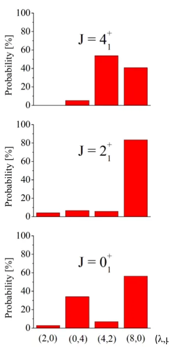
from [2]. Example of this decomposition of the first few low-lying pairing states into SU(3) basis states is given in Table 1. From this decomposition one can extract infor-mation on the intrinsic deforinfor-mation of the pairing states through the content in percentage of the SU(3) states, which are clearly associated with the (βγ) variables of the Geometric Collective Model [8]. As could be seen from Table 1 and Fig. 1, for the yrast states the prolate compo-nents (8,0) and (4,2) play a dominant role, although for the ground state they are strongly mixed with the oblate (0,4) state.
The energy of the pairing states is given by Eq. (20) in Ref. [9] where a complete classification of the states in the SO(8) proton-neutron pairing model has been done.
4 Two-parameter estimate
We start with the two parameter interaction:
H=(1−x)
2 [G0Pisc+G1Piv]− χ
2(1+x)Q.Q (5)
withG0=G1,
H= (1−x)
2 G0Pisc− χ
2(1+x)Q.Q (6)
H= (1−x)
2 G1Piv− χ
2(1+x)Q.Q (7)
Figure 1. (Color online) The structure of the pairing states for the system of 2 protons and 2 neutrons in theds-shell.
for the cases when both pairing modes are present with the same strength or when we have just the isoscalar or the isovector mode involved, respectively.
Now, let us use the energies of the low-lying states of 20O, which has 4 neutrons in thedsvalence shell. In Fig. 2,
we present the results of a minimization procedure for the
root-mean-squared valueσ= i(Ei
T h−EiExp)
2/
d( per degree of freedomd) with respect to the two parameters
Gandχof the residual interaction (5). The darker spots in the middle of the figure present the intervals of change of the parameters for which we have the minimal values ofσor the values of the parameters fitted to a set of the 12 lowest-lying positive-parity experimental energiesEi
Exp
from the observed spectra [10] of a real nuclear system. The red dashed line in Fig. 2(a) connects the values of each of the parametersGandχat their respective limit-ing cases of pure pairlimit-ing or pure quadrupole-quadrupole interactions. This line could be assigned as the axis of change of the parameter −1x1 as is used in Fig. 2(b).
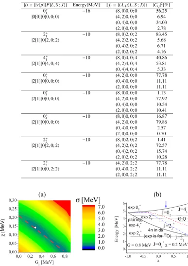
Table 1.Decomposition of the total pairing states|ΨPfor the nuclear system of 2 protons and 2 neutrons in theds-shell in terms of
SU(3) basis states|ΨR. In the first column, theJπvalue of the pairing state is given.
|i ≡ {|ν[p][P]L,S;J} Energy[MeV] |{j} ≡ {(λ, μ)L,S;J} |Ci j|2[%]
0+1 −16 (8,0)0,0; 0 56.25
|0[0][0]0,0; 0 (4,2)0,0; 0 6.94
(0,4)0,0; 0 34.03 (2,0)0,0; 0 2.78
2+1 −10 (8,0)2,0; 2 83.45
|2[1][0]2,0; 2 (4,2)2,0; 2 5.68
(0,4)2,0; 2 6.71 (2,0)2,0; 2 4.16
4+1 −10 (8,0)4,0; 4 40.86
|2[1][0]4,0; 4 (4,2)4,0; 4 53.81
(0,4)4,0; 4 5.33
0+2 −10 (4,2)0,0; 0 77.78
|2[1][0]0,0; 0 (0,4)0,0; 0 11.11 (2,0)0,0; 0 11.11
0+3 −10 (8,0)0,0; 0 1.13
|2[1][0]0,0; 0 (4,2)0,0; 0 77.92
(0,4)0,0; 0 10.54 (2,0)0,0; 0 10.41
0+4 −10 (8,0)0,0; 0 16.87
|2[1][0]0,0; 0 (4,2)0,0; 0 79.86 (0,4)0,0; 0 2.57 (2,0)0,0; 0 0.70
2+2 −10 (8,0)2,0; 2 1.41
|2[1][0]2,0; 2 (4,2)2,0; 2 72.57 (0,4)2,0; 2 15.74 (2,0)2,0; 2 10.28
2+3 −10 (4,2)0,2; 2 77.78
|2[1][0]0,2; 2 (0,4)0,2; 2 11.11
(2,0)0,2; 2 11.11
Figure 2.(Color online) Result for20O with the Hamiltonian (7). (a) The absolute RMS deviationσin MeV for the excitation spectrum
in theds-shell, calculated in full SU(3) basis. The white circle denotes the position whereσis minimal. (b) Excitation spectrum of the lowest-lying energies with the control parameterxvarying from−1 to 1 along the red line in part (a).
serve as a measure of the influence of each of the terms from the residual interactions on the energy spectra of the considered nucleus. An interesting conclusion from these two-parameter figures is that similar results forσcan be obtained by using various pairs of values (χ,G). This
cor-responds to somewhat different spectra in all these cases — from purely rotational to somewhat more pairing-like modes.
At the pairing limit (x=−1), a non-degenerateν=0,
Figure 3. (Color online) Similar to Fig. 2 but for the nucleus20Ne. Calculations are performed when (a) the total pairing or just (c)
the isoscalar or (d) the isovector part of the pairing is included in the Hamiltonian. Part (b): the excitation energies obtained with the Hamiltonian (5) with the control parameterxvarying from−1 to 1 along the red line in part (a).
J=0+1,2+1,2+2,4+1 states by the pairing gap 2Δ=GΩ. Very soon after the pairing limit, for non-vanishing values of χ first the lowest J=2+1 is separated from the rest of the degenerated excited states, then around x=0 all the states degeneracy is removed and the triplet ofν=2,J=2+1,0+2,4+1 is clearly observed, which reproduces the spectra typical for the quadrupole phonon model [11] as well as in the In-teracting Boson Model [12]. In the pure SU(3) limit (x=1), the rotational sequence ofν=2, J=0+1,2+1,4+1 states in the ground band is recovered, based on the leading SU(3) irrep (8,0) (see Table 1). As a result, a degeneracy of the two ν=2, J=2+appears, which is lifted for nonvanishing val-ues ofG. The secondν=2,J=0+2, based on leading SU(3) irrep (4,2), is the band head of the excited 0+2. It is obvious that the complicated spectra observed in real nuclear sys-tems are best reproduced by taking into account both the pairing and quadrupole-quadrupole interactions.
In the case of 20Ne (see Fig. 3), the RMS estimate is performed over the 21 lowest-lying positive-parity ex-perimental energies Ei
Exp. The results are given for the
three choices of the pairing interaction - the isoscalar, the isovector and the total pairing with a common strength pa-rameter value. For this nucleus we obtain a more rotational spectrum but again observe a flat area of minima with sim-ilar RMS values ofσ. Compared to the20O case, here the
region of values suggesting good description of the exper-iment do not reach the pure-pairing side. Also the slope of change is smaller and the point of the best description shifts to the right towards a more rotational spectrum (see the position of the blue arrow in Fig. 2(b) compared to the Fig. 3(b)).
5 Three-parameter estimate and the phase
transitions
Further, we can separate the two pairing modes – the isoscalar and the isovector one – and use a Hamiltonian of the form
H=G0VPisc+G1VPiv− χ
2Q.Q. (8)
In this case, one has to introduce two control pa-rameters y and z, described in Sec. 3.2 of Ref. [2] (see also [13]). These are defined as having the following rela-tion with the three strengthsG0,G1andχ:y=χ/(χ+G1),
z = (χ+G1)/(χ+G0 +G1) and the scaling parameter
c=χ+G0+G1. Using them, the Hamiltonian becomes
Figure 4.(Color online) A symmetry triangle that illustrates the dominance of one of the interactions: quadrupole-quadrupole, isoscalar pairing or isovector pairing. The coordinates of a point of interest areyandz. The four circles locate the results for the nuclei18Ne,18O,20Ne, and20O.
The ratio between the best-fit values for the parame-tersχ,G0andG1can be plot on a diagram resembling the Casten symmetry triangle, where each vertex represents one of the modes in pure form. The two control parame-tersyandzhave the following meaning: an angle and a distance from the point of interest to one of the vertices, respectively.
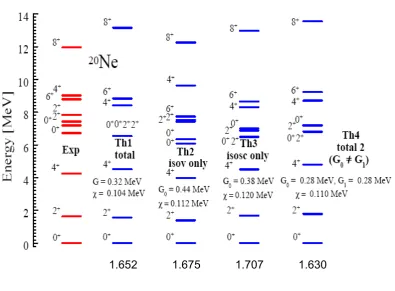
The corresponding three-parameter outcome is shown in Figs. 4 and 5. The best three-parameter results in the case of 20Ne are obtained for the values χ=0.11 MeV,
G0=0.28 MeV, and G1=0.28 MeV. The other three nu-clei in the study (18O,18Ne, and20O) have only one type of valence particles (protons or neutrons), so the three-parameter investigation is not applicable to them. We see that the best results are obtained forG0values close to the ones ofG1.
In Fig. 4, the results obtained for all 4 nuclei in our study are presented. The outcome for the nuclei18O and 18Ne has been obtained as the best two-parameter estimate
using the Hamiltonian (7). One can see that only the20Ne result for the parameters lies inside the triangle. The cases of no isoscalar pairing allowed (which is when only one type of valence particles is present in the system) lie along the SOT(5)-SU(3) line. Moreover, the more collective20O nucleus is positioned closer to the SU(3) vertex.
Finally, in Fig. 5, a comparison between excitation spectra calculated for20Ne has been done. It can be seen that the deviation from the experimental energy spectrum is reduced once one goes from two-parameter to three-parameter description. Also, the degeneracy of the states 0+2, 0+3, 2+2 and 2+3 is removed as is in the experiment.
6 Conclusion
The relation between the pairing and the quadrupole inter-action established [1, 2] on the basis of their complemen-tarity to the Wigner’s spin-isospin UST(4) symmetry was
used to elucidate the algebraic structure of an extended Pairing-plus-Quadrupole Model, realized in the frame-work of the Elliott’s SU(3) scheme [3]. The pairing part of the Hamiltonian consists ofpp-,nn- andpn-pairing terms. The relationship between the basis states classified in each of the dynamical symmetries is obtained, which allows for the evaluation of the matrix elements of the operators rep-resenting each algebra in the reductions. This approach is used to study the combined effects of the quadrupole-quadrupole and pairing interactions on the energy spectra of the nuclear systems. In a forthcoming article [14], we will describe all these effects in a sequence of N=Z nu-clei with A=2 and 4 nucleons. There, results forB(M1) andB(E2) transition strengths will also be displayed and probably included in the best fit estimate.
The phases as dynamical symmetries of an extended Pairing-plus-Quadrupole Model are investigated in the framework of the Elliott’s SU(3) scheme. The phase tran-sitions between all three limits are studied by evaluating the weights of the different interactions in the PQM Hamil-tonian for several nuclear systems with 2 and 4 particles in theds-shell. The probability distributions|Ci j|2 (transfor-mation brackets) with which the states of the SU(3) ba-sis enter into the expansion of the pairing baba-sis are ob-tained numerically. In this way, the importance (weight) of the different SU(3) - states can be used, when we need to impose restrictions on the basis because of computa-tional difficulties. The parameter adjustment for realistic nuclear systems gives the influence of each of the consid-ered pairing and quadrupole modes on the reproduction of the nuclear spectra. This evaluation is achieved and clari-fied by the introduction of two or three control parameters. The comparison of the results for different numbers and types of particles that constitute the valence shell for the nuclear system could be compared to evaluate the onset of deformation.
Acknowledgements
K.P.D. is grateful for the hospitality of the BLTP of JINR, Dubna. This work was also partially supported by the Bulgarian National Foundation for Scientific Research under Grant No. DFNI-02-6/12.12.2014.
References
[1] K.P. Drumev and A.I. Georgieva,Proc. of 32-nd Int. Workshop on Nuclear Theory (IWNT-32), eds. A.I. Georgieva, N. Minkov (Heron Press, Sofia, 2013), 151.
[2] A.I. Georgieva and K.P. Drumev, Eur. Phys. J. Web Conf., this issue.
[3] J.P. Elliott and M. Harvey, Proc. Roy. Soc. London, Ser. A272, 557 (1963); J.P. Elliott and C.E. Wilsdon, Proc. Roy. Soc. London, Ser. A302, 509 (1968) [4] C.E. Vargas, J.G. Hirsch, J.P. Draayer, Nucl. Phys. A
690, 409 (2001)
Figure 5.(Color online) Comparison of the experimental and theoretical spectra obtained for20Ne with the Hamiltonians (5), (6), (7),
and (8). Below each spectrum, the RMS value obtained is written.
[6] C. Bahri and J.P. Draayer, Comp. Phys. Commun.83, 59 (1994)
[7] C. Bahri, J. Escher, J.P. Draayer, Nucl. Phys. A592, 171 (1995)
[8] O. Castaños, J.P. Draayer, Y. Leschber, Z. Phys. A
239, 33 (1988)
[9] V.K.B. Kota and J.A. Castilho Alcarás, Nucl. Phys. A764, 181 (2006)
[10] National Nuclear Data Center, [http://www.nndc.bnl.gov].
[11] D. Janssen, R.V. Jolos, F. Dönau, Nucl. Phys. A224, 93 (1974)
[12] A. Arima and F. Iachello, Ann. Phys.99, 253 (1976) [13] J. Cseh and J. Darai, arXiv:1404.3503v1[nucl-th]
(2014)