Efficient method for transport simulations in quantum cascade lasers

Efficient method for transport simulations in quantum cascade

lasers

Mariusz Maczka1, Stanislaw Pawlowski2

1

Department of Electronics Fundamentals, Rzeszow University of Technology,W. Pola 2, 35-959 Rzeszow, Poland 2

Department of Electrodynamics and Electrical Machine Systems Rzeszow University of Technology,W. Pola 2, 35-959 Rzeszow, Poland

Abstract. An efficient method for simulating quantum transport in quantum cascade lasers is presented. The calculations are performed within a simple approximation inspired by Büttiker probes and based on a finite model for semiconductor superlattices. The formalism of non-equilibrium Green's functions is applied to determine the selected transport parameters in a typical structure of a terahertz laser. Results were compared with those obtained for a infinite model as well as other methods described in literature.

1 Introduction

Quantum cascade lasers (QCLs) are relatively new semiconductor devices [1]-[3]. Nevertheless, they have been successfully used both in scientific research [4-5] and industry applications [6] due to their properties such as high optical power output, wide tuning range of the emitted radiation and room temperature operation. QCLs have proven to be very useful for spectroscopic applications such as remote detection of dangerous gases [7], or pollutants in the atmosphere [8]. QCLs have been also proven effective in medical diagnostics where they are used as breath analyzers [9] or to study plasma chemistry [10]. Scientific studies, both theoretical and experimental, have contributed much to extending the range of their use. Many different approaches can be taken to investigate QCL theoretically. For example, the Monte Carlo method was applied in [11] to predict the current density, population inversion, and optical gain. The method used by other authors [12, 15] to calculate quantitatively QCLs parameters was a non-equilibrium Green's function method (NEGF) operating in a real space. Another known method based on Wannier functions is applied to QCL simulations [16, 17]. Infinite geometrical dimensions of the superlattice structure are assumed and periodic delocalised Bloch functions over the whole structure are considered there. It should be noted, however, that the Bloch theorem was created to describe phenomena occurring in crystal lattices, where the number of cells is incomparable with the number of semiconductor layers in the superlattice heterostructurem which are usually of several dozen, so it is difficult to properly assess the extent to which the assumed infinite dimensions of the model may affect the accuracy of QCL simulations. In [18] the authors compared the results calculated under their model to the results obtained with the finite geometrical dimensions model, and proposed Wannier-function approximation to be

used for energies close to the lowest miniband, to demonstrate accuracy of their approach. We showed [19] differences in simulation results obtained with both superlattice models, i.e. with finite and infinite geometrical dimensions, which we called finite (FM) and infinite (IM) model respectively, whereas in [20, 21] we presented a way for constructing the base of quantum states inspired by the Wannier functions base. The base we proposed used the wave functions that were the solution of the Shrödinger equation for the superlattice model of finite geometrical dimensions.

In the present study an efficient method for simulating quantum transport in QCL, based on the finite model is demonstrated. The performance of this method consists of several elements. (i) A quantum states base, inspired by Wannier functions for superlattice properties, is used which allows to limit the Hamiltonian representation solely to the space of energy [22]. For such cases nano-device Hamiltonian matrices are small, so computations run fast. (ii) The scattering process is treated as just a contact described by diagonal matrix

with phenomenological parameters η related to the

scattering time [23]. (iii) In the calculation scheme where nonequilibrium Green’s function equations are solved, a simple approximation inspired by the Büttiker probes common in mesoscopic physics is applied [23-29].

2 Superlattice Model

As mentioned in the previous chapter the finite model for simulating quantum transport in QCL is used. The main elements of this model are shown in Fig.1. It is dedicated to a quantum cascade laser, manufactured on

GaAs/Al0.15Ga0.85As superlattice base [30]. The

The model comprises the finite number n of d length modules. Each module is composed of the layers in the arrangement 7.8 / 2.4 / 6.4 / 3.8 / 14.8 / 2.4 / 9.4 / 5. Such conducting layers produce a periodic potential, which

models the energy scheme of the conduction band - EC

with the difference in values between the quantum well

bottom and the energetic barrier height ΔEC=150 meV

Fig. 1. Schematic model for a cascade laser manufactured on GaAs/Al0.15Ga0.85As superlattice base [30]. The illustrated case represents thermodynamic equilibrium.

Modelling technique for QCL is based on solving the Schrödinger equation for a variable effective mass, namely:

) ( ) ( ) ( ) (

2 2

2 2

z EΨ z

Ψ

z V dz

d z me

, (1)

where V(z) is the potential energy of the electron in the

periodic potential resulting from the superlattice semiconductor layers. The solution to equation (1) for the zj<z<zj+1 region of constant potential and constant material composition can be written as wave functions in the form:

) )( ( )

)( (

)

( j j ikj E z zj

j z z E ik j

j z A e B e

. (2)

The functions in the jth layer of the superlattice take on

the form of plane counter travelling waves with

_/ 2

2 _{j j}

j m E V

k , mj – electron effective mass, E –

total energy of an electron, Vj - the potential energy.

The wave functions for the finite superlattice model defined by expression (2) are neither localized, nor periodic [19, 20]. They are grouped within the allowed energy minibands, which are determined by non-zero transmission coefficient value:

2

1 1

1 1

A A k k

Tr L L _{, (3)}

where L stands for the total number of layers in the

structure. For expression (3) the assumption that the

electron beam concerns only the source (BL+1= 0) holds

and it determines the probability for an electron transition throughout the analyzed structure. The

transmission coefficient Tr is equal to 1 for a certain

discrete energy value of L-1 number. For the remaining

values of energy within the minibands T ranges within

0 < Tr < 1. Physically it means that the electrons of the

same miniband may have different transition probabilities for the structure, and it is believed to have a

significant impact on the assessment of its transport properties.

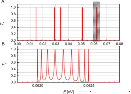
Figure 2.A shows the calculated Tr coefficient values for

the wide energy range 0-0.08 eV. Here we see a very narrow energy ranges (minibands) for which this factor has a value close to 1. A more accurate picture of the results we can be seen in Figure 2.B where narrow energy range (0.0620-0.0625 eV) is showed.

Fig. 2. The calculated values of Tr coefficient for the wide of energy range (0-0.08 eV) A) and the same values for a selected narrow energy range (0.0620-0.0625 eV).

The computation method proposed in this paper uses the base of quantum states inspired by the Wannier functions. In our case the states are maximally localised and defined for a finite model of a nonsymmetrical semiconductor superlattice. These functions were sought according to the formula:

max

min

)

,

(

)

(

E

E

dE

z

E

C

z

V

, (4)

where C is a normalization factor, which shapes the

square modulus of the function V ν to the unity of the

whole length of the structure, whereas ν indexes the

minibands.

Fig. 3. Maximally localised quantum states representing 5 lowest minibands

It should be noted that Ψν(E,z) functions are not

uniquely determined, as their particular embodiment is generally dependent on two complex constants, namely

A1- the amplitude of the wave travelling from the source

and BL+1 – amplitude of the wave travelling from the

3 The Hamiltonian of the device

Hamiltonian matrix of the device can be written as

R

H H

H ₀ where H₀ represents the sum

(

H

_SL

H

) for the cases of unpolarized and polarized

superlattices respectively, while the matrix H_R contains

all effects associated with the scattering of electrons. The

matrix of H_SL can be written as [22]:

, n, † 1, -n n, † 1, n 1 n, † n, n

SL E a a T a a a a

k k k k k k k k

H , (5)

where n is the number of the relevant period superlattice

of length d, k is the wave vector,

E

_k centre of energy

for ν miniband, T₁ represent the off-diagonal couplings

between the quantum levels in different periods, whereas

parameters †

n,

k

a and a_n,k are creation and annihilation

states operators, respectively.

The Hamiltonian matrix of the polarized structure

H

takes the form [22]:

! " " " #

, _{1 n}†_{1, n, n-}†_{1, n,}

n, † n, n, † n, 0

n e R a a a a

a a d ne a a R e

k _{k k k k}

k k k k H , (6)

where e is the electron charge, ξ is the value of the

electric field, while variable R_l" is calculated according

to the formula:

) ( ) ( * z zV ld z V dz

Rl"

" . (7)

This relationship takes into account the interaction

between both allowed minibands (indices μ, ν) and

periods (index l) of the superlattice. The Hamiltonian

matrix in our calculations included three periods of the superlattice and five maximally localized quantum states in each of them.

The transformation, described in the previous chapter, from the base of not localized wave functions to the base of maximally localized quantum states allows to reduce the Hamiltonian matrix representation from the energy-position representation to energy representation. This process is also advantageous in reducing the Hamiltonian matrix size (here 15x15), which improves the efficiency of the presented method.

In NEGF theory scattering processes expressed in

R

H

are applied in the form of self-energies as described

in the next section.

4 G

reen’s functions and self energy

approach

For calculating transport characteristics in QCL it

is necessary to use nonequilibrium, i.e. retarded GR and

correlation G<, Green’s functions to define the

nonequilibrium stationary state of the system. NEGF theory contains a description of their use for that purpose, and a self-consistent Born approximation [16] remains to be a quite popular calculation method. In this

paper we propose an approach based on other methods to determine Green’s functions. We were inspired by Büttiker probes (see Fig. 4), widely used in mesoscopic

physics, where the parameter _%bi

_$b$b

[27]

describing the exchange of electrons between the

quantum state of each module b and every reservoir of

electrons in active device, taking into account the considered scattering effects, are introduced. These

effects are included in the self-energy matrix

$

.

Fig. 4. The profile of a generic mode is illustrated along with

the placement of Büttiker probes.

For such an approach the matrix of the spectral function can be written in the form [27]:

R b N b R b N

b G Γ G

A , (8)

where N indexes all electron reservoirs. It should be

mentioned here that diagonal elements of the matrix A give information about the local density of states defined as [27]: . 2 1 2 1 2 N b R b N b

b A G Γ

D

&

&

(9)

The transmission coefficient of electrons between the

two reservoirs of m and n is determined with the

following formula [27]:

.

Trace 2 n

b R b m b R b n b R b m b mn

b Γ G Γ G Γ G Γ

T (10)

With the known local density of states, and scattering effects taken into account by the factor Γ, we can define the local concentration of electrons as [27]:

N z

N N b B b e

b F E

T k m

n

' "

&3 1/2

* , 2 1 A (11)

where F is the function of distribution of electrons,

determined by the Fermi levels μN calculated for Büttiker

probes and normalized by a factor k_BT. Similarly, the

current flowing through the probe to the quantum state b may be expressed as [27]:

, 2 2 / 1 2 / 1 3 * , 2 z n N z m mn b b B b e sB E F E F T k m e I

" " & T (12)

where the Fermi levels μn and μm of the Büttiker probes

are determined from the condition of current continuity:

0 ) (

( ( z z sB sB I E dE

This leads to an iterative equations [27]:

_,

1/2

3 * , 2 z n mn b m z m b B b e m sB mm dE E F T k m e I ! ) ) ' ' ) )

( ( T J " " &

" (14)

_,

1/2 3 * , 2 z n z n mn b b B b e n sB mn dE E F T k m e I ! ) ) ' ' ) ) ( (

" " & " T J (15)

and correction of the chemical potential at each iteration of each of the Büttiker probes in accordance with the relationship: sB sB I 1

*" J (16)

until no change of μsB occurs. Having the chemical

potential on the Büttiker probes, we can specify self

energies

Σ

R and

Σ

< as diagonal matrices with elements

in the form iη and iηfBt(E), respectively, where

exp / 1

1 )

(E E k T

fBt "zB B , while η is a

phenomenological parameter related to the scattering

time (_,/₊) [22]. The next step is to solve two kinetic

equations. The first of them is the Dyson equation [23]:

I

G

Σ

H

I

R R

E

)

(

, (17)

where _GR _{is the matrix of the retarded Green’s}

functions, which can be define as [24]:

)

(

)

(

0

,

,

lim

G

Z

E

i

E

G

R

- (18)

The second is the Keldysh equation [31]:

†

]

][

][

[

]

G

[

.

G

R

$

.

G

R , (19)

which allows to determine the correlation function

G

..

It is worth emphasizing that in the method described here, the kinetic equations (17) and (19) need to be solved only once, unlike in the Born approximation method, where they are solved repeatedly in the self-consistent process together with the equations for the self energies.

According to the assumptions made here, the density of current flowing through the laser structure, can be written just as it was for the description of the

Hamiltonian as J = J0 + JR [16], where J0 is the current

with the effects of electron scattering excluded, while JR

is a component taking then into account. As shown by the authors in [32] for the structure under consideration

the JR component disappears, and thus the total current

density can be approximated by the J0 defined as [32]:

)

(

ˆ

,

ˆ

2

2

, , , 0 , ,

E

G

z

H

dE

e

J

o .

k

k 0/ 0/

/

0

&

1

(20)

where the matrix Hˆ₀,zˆ is formed in the base of

maximally localized quantum states variable ϑ is the

volume of polarized structure. By this relationship the

density of current were calculated and the obtained results are described in the next section.

5 Calculations of G

reen’s functions

The model described in the previous chapters produced the simulations results illustrated below. In Figure 5 (left side) the imaginary diagonal elements of

the matrixes GR and G< are plotted for wave vector k=0.

There, the respective density of states (N1D(E)) and the

occupation of these states by electrons (n1D(E)) are

illustrated. The simulations were carried out with the eclectic field of 50 mV/period applied. The Fig. 5 (right side) contains also, the results of the Green’s functions calculations, using the infinite model of superlattice [33]. This juxtaposition shows differences in distribution of peak amplitudes of Green’s functions. This is a consequence of different boundary conditions used in both models.

Fig. 5. Examples of the density of states functions N1D(E) and

occupation functions n1D(E), for k=0 calculated by use Büttiker

probes, and the eclectic field of 50 mV/period applied. The simulations were carried out for the finite and the infinite models of superlattice.

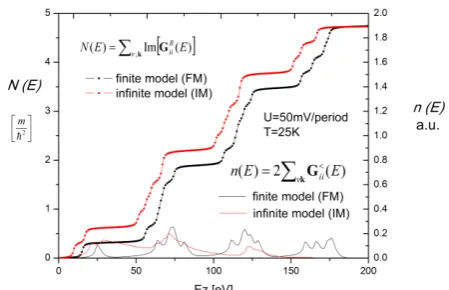
By summing up one dimensional density of states functions for all states over the selected range for the wave vector k, the function of the density of states for the three geometric dimensions (3DOS) is obtained. This

function can be written as

k G

,

3 (E) Im (E)

N R

ii

DOS .

Fig. 6. Total density of states per period N3D(E) calculated with

FM, and occupation functions per period n3D(E) calculated with Büttiker probes, and the eclectic field of 50 mV/period applied.

In a similar way we obtained the occupation function

(n3DOS(E)) for the three geometric dimensions

.

_vkG_ii

DOS E E

n3 ( ) 2 ( ). Figure 6 shows graphs of

N3DOS(E) and n3DOS(E) functions with the electric field of 50 mV/period applied. There are the results for the finite and the infinite models of superlattice.

The maps shown in Figure 7 are an extension of the results p resented in Figures 5 and 6. The density of states (Fig. 7A) and the occupation functions (Fig. 7B),

defined as

& Im(Tr([ ]))

1 ) ,

(E k_|| GR

N and

.

& Im(Tr([ ]))

2 ) ,

(E k_|| G

n respectively, are illustrated.

All these functions are shown for Büttiker probes approach, with the bias voltage of 50 mV/period applied. The results are plotted for the finite and the infinite models of superlattice, in a way that allows them to compare.

Fig.7. Density of states N(E,k||) (part A) and occupation functions n(E,k||) (part B), calculated for the bias voltage of 50 mV/period with Büttiker probes by use finite and infinite models of supperlattice.

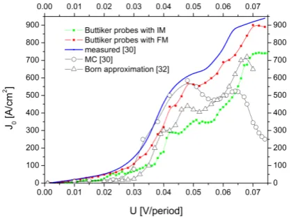
The method presented is advantageous in terms of the effectiveness of simulating U-I characteristic for QCLs. An example illustrated in Fig. 8, where the current density Jo for FM and IM models was calculated according to (20) and versus voltage polarity per period is plotted. The calculations were conducted for a superlattice temperature of 25 K [30].

Fig. 4. Current-voltage characteristics of the QCL structure [30] obtained for different approaches. The blue solid line plotted the measured current-voltage characteristics of the studied structure..

The obtained characteristics show similarity to the results presented in [32], which were calculated using the Born approximation and in [30] where we can find the measured and simulated (with Monte-Carlo (MC) method) current-voltage characteristics for the structure considered here. It seems to confirm applicability of Büttiker probes for simulating terahertz lasers with the superlattice finite model.

Summary

The theory of Büttiker probes applied to efficient calculations of the transport parameters for quantum cascade lasers, based on the finite model of superlattice, was described.

The presented simulation proved the proposed approach to have given results in line with other applicable methods described in the literature. Superiority of the developed procedure for finding laser parameters as being much faster and easier to operate in comparison to the other methods reported elsewhere was demonstrated. It gives ground for further research into the proposed approach.

References

1. J. Faist, F. Capasso, D. L. Sivco, A. L.

Hutchinson, S-N. G. Chu, A. Y. Cho, Appl. Phys. Lett. 72, 680-684 (1998)

2. R. Colombelli, F. Capasso, C. Gmachl, A. L. Hutchinson, D. L. Sivco, A. Tredicucci, M. C. Wanke, A. M. Sergent, A. Y. Cho, Appl. Phys. Lett. 78,2620 – 2622 (2001)

3. K. Kosiel, M. Bugajski, A. Szerling, J.

Kubacka-Traczyk, P. Karbownik, E.

Pruszyńska-Karbownik, J. Muszalski, A.

Łaszcz, P. Romanowski, M. Wasiak, W.

Nakwaski, I. Makarowa, P. Perlin, Photonics Letters of Poland 1, 1,16-18, (2009)

4. M. Bugajski, K. Pierściński, D. Pierścińska, A.

Szerling, K. Kosiel, Photonics Letters of Poland

5, 3, 85-87 (2013) A

5. P. Karbownik, A. Trajnerowicz, A. Szerling, A.

Wójcik-Jedlińska, M. Wasiak, E. Pruszyńska -Karbownik, K. Kosiel, I. Gronowska, R.P.

Sarzała, M. Bugajski, Optical and Quantum Electronics 47, 4, 893-899 (2015)

6. E. Normand; I. Howieson; M. T. McCulloch, Laser Focus World 43 4, 90–92 (April 2007)

7. Z. Bielecki, J. Wojtas, T. Stacewicz,

Elektronika-Konstrukcje-Technologie-Zastosowania, 11, 44 (2014)

8. M. Miczuga, K. Kopczyński, J. Pietrzak,

Elektronika-Konstrukcje-Technologie-Zastosowania, 11, 47 (2014)

9. M. Hannemann, A. Antufjew, K. Borgmann, F.

Hempel, T. Ittermann, S Welzel., K.D.

Weltmann, H. Völzke, J. Röpcke , Journal of Breath Research, 5 ,027101 (2011)

10. N. Lang; J.Röpcke; S. Wege; A. Steinach, Eur. Phys. J. Appl. Phys.49, 13110:3 (2009)

11. E. Bellotti, K. Driscoll, T. D. Moustakas and R. Paiella, Journal of Applied Physics 105, 11 (2009)

12. S. Birner, T. Zibold, T. Andlauer, T. Kubis, M. Sabathil, A. Trellakis, P. Vogl, IEEE Transactions on Electron Devices 54, 9, 2137 (2007)

13. T. Kubis, C. Yeh, and P. Vogl, Phys. Rev. B

79, 19, 195323-1–195323-10 (2009)

14. G. Hałdaś, A. Kolek, and I. Tralle, Journal of Quantum Electronics 47, 6 (2011)

15. A. Kolek, G. Hałdaś, M. Bugajski, Appl. Phys. Lett. 101, 061110 (2012)

16. S.-C. Lee and A. Wacker, Phys. Rev. B 66, 245314 (2002)

17. A. Wacker, S.-C. Lee, M.F. Pereira Jr, Advances in Solid State Physics ed. by B. Kramer 43, Springer, Berlin, 369–380 (2003) 18. A. Wacker and B. Y.-K. Hu, Phys. Rev. B 60,

23, 16039-16049 (1999)

19. M. Mączka, S. Pawłowski, J. Plewako,

Electrical Review 8, 93 (2011)

20. S. Pawłowski, M. Mączka, Przegląd

Elektrotechniczny 11, 322-327 (2013)

21. M. Mączka, S. Pawłowski, Przegląd

Elektrotechniczny 12, 245 (2013)

22. A. Wacker, Physics Reports 357, 1-111 (2002) 23. S. Datta, Phys. Rev. B40, 5830 (1989)

24. S. Datta, Electronic transport in mesoscopic systems (Cambridge University Press, 1995) 25. MBüttiker, Phys. Rev. Lett. 57, 1761 (1986) 26. Texier and M. Büttiker,Phys. Rev. B 62, 7454

(2000)

27. R.Venugopal, M. Paulsson, S. Goasguen, S. Datta, and M. Lundstrom, J. Appl. Phys. 93, 5613 (2003)

28. P. Greck, S. Birner, B. Huber, P. Vog, Optics Express 23, 6587-6600 (2015)

29. M. Mączka, Przegląd Elektrotechniczny, 7,

190-196 (2016)

30. H. Callebaut and Hu Q., J. Appl. Phys. 98, 104505 (2005)

31. L. V. Keldysh, Sov. Phys. JETP 20, 4, 1018–

1026 (1965)

32. S.-C. Lee, F. Banit, M. Woerner, and A. Wacker, Phys. Rev. B 73, 245320 (2006) 33. M. Mączka, S. Pawłowski, Elektronika