Mod´elisation Math´ematique et Analyse Num´erique M2AN, Vol. 36, No5, 2002, pp. 747–771 DOI: 10.1051/m2an:2002035
A MATHEMATICAL AND COMPUTATIONAL FRAMEWORK FOR RELIABLE
REAL-TIME SOLUTION OF PARAMETRIZED PARTIAL DIFFERENTIAL
EQUATIONS
Christophe Prud’homme
1, Dimitrios V. Rovas
1, Karen Veroy
1and
Anthony T. Patera
1Abstract. We present in this article two components: these components can in fact serve various goals independently, though we consider them here as an ensemble. The first component is a technique for therapid and reliable evaluationprediction of linear functional outputs of elliptic (and parabolic) partial differential equations with affine parameter dependence. The essential features are (i) (prov-ably) rapidly convergent global reduced–basis approximations — Galerkin projection onto a spaceWN spanned by solutions of the governing partial differential equation atN selected points in parameter space; (ii)a posteriorierror estimation — relaxations of the error–residual equation that provide inex-pensive yet sharp and rigorous bounds for the error in the outputs of interest; and (iii) off–line/on–line computational procedures — methods which decouple the generation and projection stages of the ap-proximation process. This component is ideally suited — considering the operation count of the online stage — for the repeated and rapid evaluation required in the context of parameter estimation, design, optimization, and real–time control. The second component is a framework for distributed simulations. This framework comprises a library providing the necessary abstractions/concepts for distributed sim-ulations and a small set of tools — namely SimTEXandSimLaB— allowing an easy manipulation of
those simulations. While the library is the backbone of the framework and is therefore general, the various interfaces answer specific needs. We shall describe both components and present how they interact.
Mathematics Subject Classification. 65N15, 65N30, 68U01, 68U20, 68M14, 68M15. Received: 23 January, 2002. Revised: 4 June, 2002.
1.
Introduction to reduced basis output bound methods
The optimization, control, and characterization of an engineering component or system requires the predic-tion of certain “quantities of interest”, or performance metrics, which we shall denote outputs— for example deflections, maximum stresses, maximum temperatures, heat transfer rates, flowrates, or lift and drags. These outputs are typically expressed as functionals of field variables associated with a parametrized partial differ-ential equation which describes the physical behavior of the component or system. The parameters, which we
Keywords and phrases.Mathematical framework, reduced-basis methods, error bounds, computational framework, simulations repository, distributed and parallel computing, CORBA, C++.
1 Massachusetts Institute of Technology, Department of Mechanical Engineering, Room 3-266, 77 Massachusetts Ave.,
Cambridge, MA 02139, USA. e-mail: [email protected]
c
shall denoteinputs, serve to identify a particular “configuration” of the component: these inputs may represent design or decision variables, such as geometry — for example, in optimization studies; control variables, such as actuator power — for example in real–time applications; or characterization variables, such as physical proper-ties — for example in inverse problems. We thus arrive at an implicitinput–outputrelationship, evaluation of which demands solution of the underlying partial differential equation.
Our goal is the development of computational methods that permit rapid and reliable evaluation of this partial-differential-equation-induced input-output relationship in the limit of many queries — that is, in the design, optimization, control, and characterization contexts. The “many query” limit has certainly received considerable attention: from “fast loads” or multiple right-hand side notions (e.g.[5, 7]) to matrix perturbation theories (e.g.[1, 25]) to continuation methods (e.g.[2, 20]). Our particular approach is based upon the reduced– basis method, first introduced in the late 1970s for nonlinear structural analysis [3, 13], and subsequently developed more broadly in the 1980s and 1990s [4, 8, 16, 17, 21]. The reduced–basis method recognizes that the field variable is not, in fact, some arbitrary member of the infinite-dimensional space associated with the partial differential equation; rather, it resides, or “evolves”, on a much lower–dimensional manifold induced by the parametric dependence.
The reduced–basis approach as earlier articulated is local in parameter space in both practice and theory. To wit, Lagrangian or Taylor approximation spaces for the low–dimensional manifold are typically defined relative to a particular parameter point; and the associateda priori convergence theory relies on asymptotic arguments in sufficiently small neighborhoods [8]. As a result, the computational improvements — relative to conventional (say) finite element approximation — are quite modest [17]. Our work differs from these earlier efforts in several important ways: first, we develop (in some cases, probably)globalapproximation spaces; second, we introduce rigorous a posteriori error estimators; and third, we exploit off–line/on–line computational decompositions. These three ingredients allow us — for a restricted but important class of problems — to reliably decouple the generation and projection stages of reduced–basis approximation, thereby effecting computational economies of several orders of magnitude.
In this expository review paper we focus on these new ingredients. We begin in Section 2 by introducing an abstract problem formulation and several illustrative instantiations. In Section 3 we describe the reduced–basis approximation for coercive symmetric problems and “compliant” outputs; associated a posteriori estimators are then developed in Section 4.
2.
Problem statement
2.1.
Abstract formulation
We consider a suitably regular domain Ω⊂Rd,d= 1, 2,or 3, and associated function space X ⊂H1(Ω), where H1(Ω) ={v ∈L2(Ω), ∇v ∈ (L2(Ω))d}, and L2(Ω) is the space of square integrable functions over Ω. The inner product and norm associated withX are given by (·,·)Xand·X= (·,·)1/2, respectively. We also define a parameter setD ∈RP, a particular point in which will be denotedµ. Note that Ω doesnot depend on the parameter.
We then introduce a bilinear form a: X ×X× D → R, and linear forms f: X → R, : X → R. We shall assume that ais continuous,a(w, v;µ) ≤ γ(µ) wX vX ≤γ0 wX vX, ∀µ∈ D; furthermore, in Sections 3 and 4, we assume thatais coercive,
0< α0≤ α(µ) = inf w∈X
a(w, w;µ)
w2X , ∀µ∈ D, (1)
We shall also make certain assumptions on the parametric dependence ofa,f, and. In particular, we shall suppose that, for some finite (preferably small) integerQ,amay be expressed as
a(w, v;µ) = Q
q=1
σq(µ)aq(w, v), ∀ w, v∈X, ∀µ∈ D, (2)
for some σq: D → R and aq: X ×X → R, q = 1, . . . , Q. This “separability”, or “affine”, assumption on the parameter dependence is crucial to computational efficiency; however, certain relaxations are possible — see [19]. For simplicity of exposition, we assume that f and do not depend on µ; in actual practice, affine dependence is readily admitted.
Our abstract problem statement is then: for anyµ∈ D, findu(µ)∈X such that
a(u(µ), v;µ) = f(v), ∀v∈X; (3)
ands(µ)∈Rgiven by
s(µ) =(u(µ)). (4)
In the language of the introduction, ais our partial differential equation (in weak form), µis our parameter,
u(µ) is our field variable, ands(µ) is our output.
For simplicity, we may suppress theµ-dependence along the article when there is no possible confusion.
2.2.
Particular instantiations
We indicate here a few instantiations of the abstract formulation; these will serve to illustrate the methods (for coercive, symmetric problems) of Sections 3 and 4.
2.2.1. A thermal fin
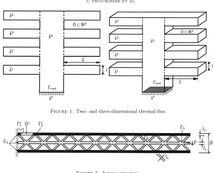
In this example we consider the two- and three-dimensional thermal fins shown in Figure 1; these examples may be (interactively) accessed on our web site1. The fins consist of a vertical central “post” of conductivity ˜k0
and four horizontal “subfins” of conductivity ˜ki, i= 1, . . . ,4; the fins conduct heat from a prescribed uniform flux source, ˜q, at the root, ˜Γroot, through the post and large-surface-area subfins to the surrounding flowing air; the latter is characterized by a sink temperature ˜u0, and prescribed heat transfer coefficient ˜h. The physical model is simple conduction: the temperature field in the fin, ˜u, satisfies
4
i=0
˜ Ωi
˜
ki ∇˜u˜·∇˜˜v +
∂Ω˜\˜Γroot
˜
h(˜u−u˜0) ˜v =
˜Γroot
˜
qv,˜ ∀v˜∈X˜ ≡H1( ˜Ω), (5)
where ˜Ωi is that part of the domain with conductivity ˜ki, and∂Ω denotes the boundary of ˜˜ Ω.
We now (i) nondimensionalize the weak equations (5), and (ii) apply a continuous piecewise-affine transfor-mation to map ˜Ω to a fixed reference domain Ω [10]. The abstract problem statement (3) is then recovered [22] forµ={k1, k2, k3, k4, Bi, L, t},D= [0.1,10.0]4×[0.01,1.0]×[2.0,3.0]×[0.1×0.5], andP= 7; herek1, . . . , k4
are the thermal conductivities of the “subfins” (see Fig. 1) relative to the thermal conductivity of the fin base; Bi is a nondimensional form of the heat transfer coefficient; and, L, tare the length and thickness of each of the “subfins” relative to the length of the fin root ˜Γroot. It is readily verified that a is continuous, coercive, and symmetric; and that the “affine” assumption (2) obtains for Q= 16 (two-dimensional case) and Q= 25 (three-dimensional case). Note that the geometric variations are reflected,viathe mapping, in theσq(µ).
Figure 1. Two- and three-dimensional thermal fins.
Figure 2. A truss structure.
For our output of interest,s(µ), we consider the average temperature of the root of the fin nondimensionalized relative to ˜q, ˜k0, and the length of the fin root. This output is calculated ass(µ) = (u(µ)), where (v) =
Γrootv. It is readily shown that this output functional is bounded and also “compliant”: (v) =f(v), ∀v∈X.
2.2.2. A truss structure
We consider a prismatic microtruss structure [6, 24] shown in Figure 2; this example may be (interactively) accessed on our web site2. The truss consists of a frame (upper and lower faces, in dark gray) and a core (trusses and middle sheet, in light gray); the structure transmits a force per unit depth ˜F uniformly distributed over the tip of the middle sheet, ˜Γ3, through the truss system to the fixed left wall, ˜Γ0. The physical model is simple plane–strain (two-dimensional) linear elasticity: the displacement fieldui, i= 1,2,satisfies
˜ Ω
∂v˜i
∂x˜j ˜
Eijkl∂u˜k ∂x˜l
=−
˜
F
˜
tc ˜Γ3v˜2, ∀ v∈
˜
X, (6)
where ˜Ω is the truss domain, and ˜X refers to the set of functions in H1( ˜Ω) which vanish on ˜Γ0. We assume summation over repeated indices.
We now (i) nondimensionalize the weak equations (6), and (ii) apply a continuous piecewise-affine transfor-mation to map ˜Ω to a fixed reference domain Ω. The abstract problem statement (3) is then recovered [23] for µ ={tf, tt, H, θ},D = [0.08,1.0]×[0.2,2.0]×[4.0,10.0]×[30.0◦,60.0◦], and P = 4; here tf and tt are
the thicknesses of the frame and trusses, respectively; H is the total height of the microtruss; and θ is the angle between the trusses and the faces. The Poisson’s ratio,ν = 0.3, and the frame and core Young’s moduli,
Ef = 75 GPa andEc = 200 GPa, respectively, are held fixed. It is readily verified thatais continuous, coercive, and symmetric; and that the “affine” assumption (2) obtains forQ= 44;Qis larger than for the fin examples due to the more complex (sheared) affine geometry mappings.
Our outputs of interest are (i) the average downward deflection (compliance) at the core tip, Γ3, nondi-mensionalized by ˜F /E˜f; and (ii) the average normal stress across the critical (yield) section denoted Γs1 in Figure 2. These compliance and noncompliance outputs are written ass1(µ) =1(u(µ)) ands2(µ) =2(u(µ)), respectively, where1(v) =−Γ
3v2, and
2(v) = 1
tf
Ωs ∂χi
∂xjEijkl ∂uk
∂xl
are bounded linear functionals; here χi is any suitably smooth function in H1(Ωs) such thatχiˆni = 1 on Γs1 andχiˆni= 0 on Γs2, where ˆnis the unit normal.
3.
Reduced-basis approach
We recall that in this section, as well as in Section 4, we assume that ais continuous, coercive, symmetric, and affine in µ— see (2); and that(v) =f(v), which we denote “compliance”.
3.1.
Reduced-basis approximation
We first introduce a sample in parameter space, SN = {µ1, . . . , µN}, where µi ∈ D, i = 1, . . . , N; see Section 3.2 for a brief discussion of point distribution. We then define our Lagrangian [17] reduced–basis approximation space as WN = span{ζn ≡u(µn), n = 1, . . . , N}, where u(µn) ∈X is the solution to (3) for
µ=µn. In actual practice,u(µn) is replaced by a finite element approximation on a suitably fine truth mesh; we shall discuss the associated computational implications in Section 3.3. Our reduced–basis approximation is then: for anyµ∈ D, finduN(µ)∈WN such that
a(uN(µ), v;µ) = (v), ∀ v∈WN; (7)
we then evaluatesN(µ) =(uN(µ)). (Non-Galerkin projections are briefly described in [19].)
3.2.
A priori
convergence theory
3.2.1. Optimality
We consider here the convergence rate of uN(µ) → u(µ) and sN(µ) → s(µ) asN → ∞. To begin, it is standard to demonstrate optimality ofuN(µ) in the sense that
u(µ)−uN(µ)X≤
γ(µ)
α(µ) wNinf∈WN
u(µ)−wNX. (8)
We note that, in the coercive case, stability of our “conforming” discrete approximation is not an issue; the noncoercive case is decidedly more delicate (see [19]). Furthermore, for our compliance output,
s(µ) =sN(µ) +(u−uN) =sN(µ) +a(u, u−uN;µ) =sN(µ) +a(u−uN, u−uN;µ) (9)
3.2.2. Best approximation
It now remains to bound the dependence of the error in the best approximation as a function of N. At present, the theory is restricted to the case in which P= 1, D= [0, µmax], and
a(w, v;µ) =a0(w, v) +µa1(w, v), (10)
where a0 is continuous, coercive, and symmetric, and a1 is continuous, positive semi-definite (a1(w, w) ≥0, ∀w∈X), and symmetric. This model problem (10) is rather broadly relevant, for example to variable orthotropic conductivity, rectilinear geometry variations, piecewise-constant conductivity variations, and variable Robin boundary conditions.
We now suppose that theµn, n= 1, . . . , N, are logarithmically distributed in the sense that
ln
µn+λ−1
= lnλ−1+ n−1
N−1 ln
µmax +λ−1
λ−1
, n= 1, . . . , N, (11)
whereλis the maximum eigenvalue ofa0relative toa1. (Noteλis perforce bounded thanks to our assumption of continuity and coercivity; the possibility of a continuous spectrum does not, in practice, pose any problems.) We can then prove [12] that, forN > Ncrit≡2eln(λ µmax+ 1),
inf wN∈WN
u(µ)−wN(µ)X ≤ γ
αu(0)X exp
−N
2eln(λ µmax+ 1)
, ∀µ∈ D. (12)
We observe exponential convergence, uniformly (globally) for all µ in D, with only very weak (logarithmic) dependence on the range of the parameter (µmax).
The proof exploits the (parameter–space) interpolant as a surrogate for the Galerkin approximation. As a result, the bound is not “sharp”: we observe many cases in which the Galerkin projection is considerably better than the associated interpolant; optimality (8) chooses to “illuminate” only certain points µn, automatically selecting a best “sub–approximation” amongst all possibilities — we thus see why reduced–basis state-space
approximation of s(µ) via u(µ) is preferred to simple parameter-space interpolation of s(µ) (“connecting the dots”)via(µn, s(µn)) pairs. Nevertheless, the logarithmic point distribution (11) implicated by our interpolant– based arguments isnotsimply an artifact of the proof: in numerous numerical tests, the logarithmic distribution performs considerably better than other obvious candidates, in particular for large ranges of the parameter. Fortunately, the convergence rate is not toosensitive to point selection: the theory only requires a log “on the average” distribution [12]; and, in practice,λin (12) may be replaced with any “reasonable” value.
Table 1. Error, error bound, and effectivity as a function ofN, at a particular representative
pointµ∈ D, for the two-dimensional thermal fin problem (compliant output).
N |s(µ)−sN(µ)|/s(µ) ∆N(µ)/s(µ) ηN(µ) 10 1.29×10⁻² 8.60×10⁻² 2.85 20 1.29×10⁻³ 9.36×10⁻³ 2.76 30 5.37×10⁻⁴ 4.25×10⁻³ 2.68 40 8.00×10⁻⁵ 5.30×10⁻⁴ 2.86 50 3.97×10⁻⁵ 2.97×10⁻⁴ 2.72 60 1.34×10⁻⁵ 1.27×10⁻⁴ 2.54 70 8.10×10⁻⁶ 7.72×10⁻⁵ 2.53 80 2.56×10⁻⁶ 2.24×10⁻⁵ 2.59
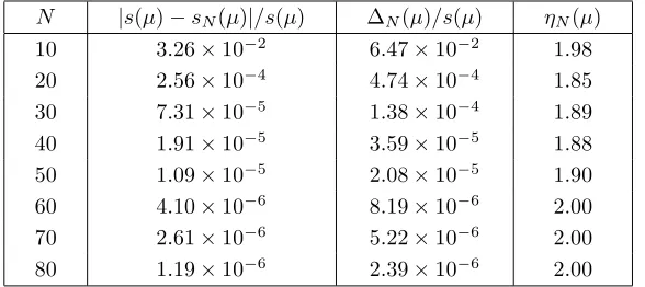
Table 2. Error, error bound, and effectivity as a function ofN, at a particular representative
pointµ∈ D, for the truss problem (compliant output).
N |s(µ)−sN(µ)|/s(µ) ∆N(µ)/s(µ) ηN(µ) 10 3.26×10⁻² 6.47×10⁻² 1.98 20 2.56×10⁻⁴ 4.74×10⁻⁴ 1.85 30 7.31×10⁻⁵ 1.38×10⁻⁴ 1.89 40 1.91×10⁻⁵ 3.59×10⁻⁵ 1.88 50 1.09×10⁻⁵ 2.08×10⁻⁵ 1.90 60 4.10×10⁻⁶ 8.19×10⁻⁶ 2.00 70 2.61×10⁻⁶ 5.22×10⁻⁶ 2.00 80 1.19×10⁻⁶ 2.39×10⁻⁶ 2.00
3.3.
Computational procedure
The theoretical and empirical results of Sections 3.1 and 3.2 suggest that N may, indeed, be chosen very small. We now develop off–line/on–line computational procedures that exploit this dimension reduction.
We first expressuN(µ) as
uN(µ) = N
j=1
uN j(µ)ζj = (uN(µ))T ζ, (13)
where uN(µ) ∈ RN; we then choose for test functions v = ζ
i, i = 1, . . . , N. Inserting these representations into (7) yields the desired algebraic equations foruN(µ)∈RN,
AN(µ)uN(µ) = FN (14)
We now invoke (2) to write
AN i,j(µ) =a(ζj, ζi;µ) = Q
q=1
σq(µ)aq(ζj, ζi), (15)
or
AN(µ) = Q
q=1
σq(µ)AqN,
whereAqN i,j=aq(ζj, ζi),i≤i, j≤N, 1≤q≤Q. The off–line/on–line decomposition is now clear:
In theoff–line stage, we compute the u(µn) and form the AqN and FN: this requiresN (expensive) “a” finite element solutions andO(QN2) finite-element-vector inner products.
In the on–line stage, for any given new µ, we first formAN from (15), then solve (14) foruN(µ), and finally evaluatesN(µ) =FTNuN(µ): this requiresO(QN2) +O(23N3) operations andO(QN2) storage. Thus, as required, the incremental, or marginal, cost to evaluatesN(µ) for any given newµ— as proposed in a design, optimization, or inverse-problem context — is very small: first, becauseN is very small, typicallyO(10) — thanks to the good convergence properties ofWN; and second, because (14) can be very rapidly assembled and inverted — thanks to the off–line/on–line decomposition. For the problems discussed in this paper, the resulting computational savings relative to standard (well-designed) finite-element approaches are significant — at leastO(10), typicallyO(100), and oftenO(1000) or more.
4.
A POSTERIORIerror estimation: Output bounds
From Section 3 we know that, in theory, we can obtain sN(µ) very inexpensively: the on–line stage scales as O(N3) +O(QN2); andN can,in theory, be chosen quite small. However,in practice, we do not knowhow
small N can be chosen: this will depend on the desired accuracy, the selected output(s) of interest, and the particular problem in question; in some cases N = 5 may suffice, while in other cases,N = 100 may still be insufficient. In the face of this uncertainty, either too many or too few basis functions will be retained: the former results in computational inefficiency; the latter in unacceptable uncertainty — particularly egregious in the decision contexts in which reduced–basis methods typically serve. We thus needa posteriorierror estimators forsN. Surprisingly,a posteriorierror estimation has received relatively little attention within the reduced–basis framework [13], even though reduced–basis methods are particularly in need of accuracy assessment: the spaces aread hocand pre-asymptotic, admitting relatively little intuition, “rules of thumb,” or standard approximation notions.
Recall that, in the section, we continue to assume thatais coercive and symmetric, andis “compliant”.
4.1.
Method I
The approach described in this section is a particular instance of a general “variational” framework for
a posteriori error estimation of outputs of interest. However, the reduced-basis instantiation described here differs significantly from earlier applications to finite element discretization error [9, 11] and iterative solution error [14, 15] both in the choice of (energy) relaxation and in the associated computational artifice.
4.1.1. Formulation
We assume that we are given a function g(µ) : D → R+, and a continuous, coercive, symmetric (µ -independent) bilinear form ˆa:X×X →R, such that
We then find ˆe(µ)∈X such that
g(µ) ˆa(ˆe(µ), v) = R(v;uN(µ);µ), ∀v∈X (17)
where for a givenw∈X,R(v;w;µ) =(v)−a(w, v;µ) is the weak form of the residual. Our lower and upper output estimators are then evaluated as
s−N(µ) ≡ sN(µ),andsN+(µ)≡sN(µ) + ∆N(µ), (18)
respectively, where
∆N(µ) ≡ g(µ) ˆa(ˆe(µ),ˆe(µ)) (19)
is the estimator gap.
4.1.2. Computational procedure
Finally, we turn to the computational artifice by which we can efficiently compute ∆N(µ) in the on–line stage of our procedure. To begin, we rewrite the “modified” error equation, (17), as
ˆ
a(ˆe(µ), v) = 1
g(µ)
(v)− Q q=1 N j=1
σq(µ)uN j(µ)aq(ζj, v)
, ∀v∈X
where we have appealed to our reduced–basis approximation (13) and the affine decomposition (2). It is immediately clear from linear superposition that we can express ˆe(µ) as
ˆ
e(µ) = 1
g(µ)
zˆ0+
Q q=1 N j=1
σq(µ)uN j(µ)ˆzjq
; (20)
where ˆz0 ∈X satisfies ˆa(ˆz0, v) = (v), ∀ v ∈X, and ˆzjq ∈ X, j= 1, . . . , N, q = 1, . . . , Q, satisfies ˆa(ˆzjq, v) = −aq(ζj, v), ∀v∈X.Inserting (20) into our expression for the upper bound,s+N(µ) =sN(µ) +g(µ)ˆa(ˆe(µ),eˆ(µ)), we obtain
s+N(µ) =sN(µ) + 1
g(µ)
c0+ 2 Q q=1 N j=1
σq(µ)uN j(µ)Λqj + Q
q=1 Q
q=1 N
j=1 N
j=1
σq(µ)σq(µ)uN j(µ)uN j(µ)Γqq jj
(21)
where c0 = ˆa(ˆz0,zˆ0), Λqj = ˆa(ˆz0,zˆqj), and Γqqjj = ˆa(ˆzqj,ˆzqj). The off–line/on–line decomposition should now be clear.
In theoff–line stage we compute ˆz0 and ˆzjq, j = 1, . . . , N, q= 1, . . . , Q, and then formc0,Λqj, and Γqqjj:
this requires QN+ 1 (expensive) “ˆa” finite element solutions, and O(Q2N2) finite-element-vector inner products.
In the on–line stage, for any given new µ, we evaluates+N as expressed in (21): this requires O(Q2N2) operations; andO(Q2N2) storage (forc0, Λqj, and Γqqjj).
As for the computation of sN(µ), the marginal cost for the computation ofs±N(µ) for any given newµis quite small — in particular, independent of the dimension of the truth finite element approximation spaceX.
for example,WN
j may contain the N
j sample points ofSN closest to the newµof interest — until ∆Nj is less than a specified error tolerance. This procedure both minimizes the on–line computational effort and reduces conditioning problems — while simultaneously ensuring accuracy and certainty.
4.2.
Method II
As already indicated, Method I has certain limitations; we discuss here a Method II which addresses these limitations — albeit at the loss of complete certainty.
4.2.1. Formulation
To begin, we set M > N, and introduce a parameter sampleSM ={µ1, . . . , µM} and associated reduced– basis approximation spaceWM = span{ζm≡u(µm), m= 1, . . . , M}; both for theoretical and practical reasons we requireSN ⊂SM and thereforeWN ⊂WM. The procedure is very simple: we first finduM(µ)∈WM such thata(uM(µ), v;µ) =f(v),∀v∈WM; we then evaluatesM(µ) =(uM(µ)); and, finally, we compute our upper and lower output estimators as
s−N,M(µ) =sN(µ), sN,M+ (µ) =sN(µ) + ∆N,M(µ), (22)
where ∆N,M(µ), the estimator bound gap, is given by
∆N,M(µ) = 1
τ(sM(µ)−sN(µ)) (23)
for someτ ∈(0,1). The effectivity of the approximation is defined as
ηN,M(µ) =
∆N,M(µ)
s(µ)−sN(µ)·
(24)
For our purposes here, we shall considerM = 2N.
4.2.2. Computational procedure
Since the error bounds are based entirely on evaluation of the output, we can directly adapt the off–line/on– line procedure of Section 3.3. Note that the calculation of the output approximation sN(µ) and the output bounds are now integrated: AN(µ) andFN(µ) (yieldingsN(µ)) are a sub-matrix and sub-vector ofA2N(µ) and
F2N(µ) (yieldings2N(µ), ∆N,2N(µ) ands±N,2N(µ)) respectively.
In theoff–linestage, we compute theu(µn) and form theA2qN andF2N: this requires 2N (expensive) “a” finite element solutions, andO(4QN2) finite-element-vector inner products.
In theon–linestage, for any given newµ, we first formAN(µ) andA2N(µ) then solve foruN(µ) andu2N(µ), and finally evaluates±N,2N(µ): this requiresO(4QN2) +O(163N3) operations andO(4QN2) storage.
The on–line effort for this Method II predictor/error estimator procedure (based onsN(µ) ands2N(µ)) will require eightfold more operations than the predictor procedure of Section 4.1.
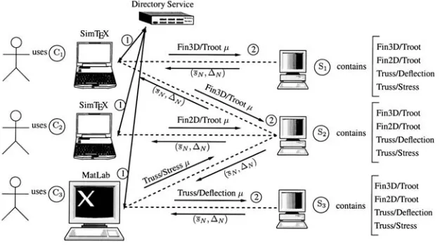
Figure 3. A sample use case of the framework.
5.
System architecture
5.1.
Introduction
The numerical methods proposed are rather unique relative to more standard approaches to partial dif-ferential equations. Reduced–basis output bound methods — in particular the global approximation spaces,a posteriorierror estimators, and off–line/on–line computational decomposition — are intended to render partial– differential-equation solutions truly “useful”: essentially real–time as regards operation count; “blackbox” as regards reliability; and directly relevant as regards the (limited) input–output data required. But to be truly useful, the methodology — in particular the inventory of on–line codes — must reside within a special frame-work. This framework must permit a User to specify — within a native applications context — the problem, output, and input value of interest; and to receive — quasi–instantaneously — the desired prediction and cer-tificate of fidelity (error bound). We describe such a (fully implemented, fully functional) framework here: we focus primarily on the User point of view; see [18] for a more detailed description of the technical foundations and ingredients.
5.2.
Overview of framework
We show in Figure 3 a virtual schematic of the framework. The key components are the User, Computers, Network, Client software, Server software, and Directory Service. Each User interacts with the system through a selected Client (interface) which resides, say, on the User’s Computer; we shall describe briefly below two Clients. Based on directives from the User, the Client broadcasts over the Network a Problem Label (e.g.
Fin3D), Output Label (e.g. Troot) Pair. This Pair is received by the Directory Service — a White Pages — which informs the Client of the Simulation Resource Locator “SRL” — physical location on a particular Computer — of a Server which can respond to the request. The Client then sends the Input (µ P–tuple Value) to the designated SRL. The Server — essentially a suite of on–line codes and associated input–output utilities — is awaiting queries at all times; upon receipt of the Input it executes the on–line code for the designated Output Label and Input Value, and responds to the Client with the Output Value (sN) and Error Bound Gap (∆N). The Client then displays or acts upon this information, and the cycle is complete.
the calculations over multiple (e.g. as many as L) Servers — in particular Servers on multiple Computers — so as respond more quickly to this multiple–input query. Our framework is clearly an example of “grid” computing, similar to GLOBUS, NetSolve, and Seti@HOME, to name but a few. Indeed, we exploit several generic tools upon which grid and network computing applications may be built; for example, we appeal to CORBA3 (standardized by OMG4) to seamlessly manipulate the Server softwareas if it resided on the Client Computer. We remark that our reduced–basis output bound application is particularly well–suited to grid computing: the computational load on participating Computers (on which the Servers reside) is very light; and the Client–Server input/output load on the Network is very light. The network computing paradigm also serves very well the archival, collaboration, and integration aspects of standardized input–output objects.
5.3.
Clients
We describe here two Clients: SimTEX, which is a PDF–based “dynamic text” interface for interrogation,
exploration, and display; andSimLaB, which is a MATLAB–based “mathematical” interface for manipulation
and integration. A third client has been developed: WebLaB; however it is a direct application of theMatLaB
client using theMatLaBWeb Server Toolbox.
5.3.1. SimTEX
SimTEXcombines several standardized tools so as to provide a very simple interface by which to access the
Servers. A particularly nice feature of SimTEXis the natural context which it provides — in essence, defining
the input–output relationship and problem definition in the language of the application. The SimTEX Client
should prove useful in a number of different contexts: textbooks and technical manuscripts; handbooks; and product specification and design sheets.
The SimTEX Client consists of an authoring component, a display and interface component, and an
“in-termediary” component. The authoring component is — a standard in scientific typesetting — enhanced (via
hyperref) with a new acteqenvironment which permits the inclusion of actionable equations. The acteq environment links an equation to a Problem Label, Output Label(s) and Input Value template. The output is a PDFdocument: thePDFdocument serves as the display, graphics, and (rudimentary) interface component
of SimTEX. ThePDFdocument contains a form which accepts the Input Values, and an “equal sign” button
which initiates the Client–Directory Services Client–Server dialogue described in the previous document. Upon completion of the cycle, thePDFdocument is updated to display the values of the output and error bound for
the Input Values submitted; in cases in which multiple input values or outputs are selected, appropriate graphics are presented using theFigurebutton. Finally, sincePDFis not a programming language, and Client–Server
intermediary is required: a CGI script serves to parse thePDFform, communicate with the Server, and finally
update the Client.
As an example, we include here an actionable equation — the actual SimTEX user interface — for the
several outputs (the root temperature, tip temperature, volume) associated with the three–dimensional thermal fin example:
The input list corresponds to theµvector described in Section 2.2.1; the input values must lie in the parameter domain D described in Section 2.2.1. The notation Output = F(Input) is a description of the input–output relationships(µ) implied bys=(u(µ)). The actionablePDFversion of this entire paper (in which is embedded
the actionable equation) may be found on our web site5; readers are encouraged to access this electronic version of the paper and exercise theSimTEXinterface, a brief users manual for which may be found again on our web
site6.
5.3.2. SimLaB
The main drawback of SimTEXis the inability to manipulate the on–line codes. SimLaBis a suite of tools
that permit Users to incorporate Server on–line codes as MATLAB functions within the standard MATLAB interface; and to generate new Servers and on–line codes from standard MATLAB functions (which themselves may be built upon other on–line codes). In short,SimLaBpermits the User to treat the inputs and outputs of
our on–line codes as mathematical objects that are the result of, or an argument to, other functions — graphics, system design, or optimization — and to archive these higher level operations in new Server objects available to all Clients once registered in the Directory Service.
For example, to incorporate the Fin3D input–output relationship into MATLAB, we first generate the needed MATLAB functions using a MATLAB script called st2m. This script, by default, generates automatically a MATLAB function for each Output registered in the Directory Service. It is also possible to ask for a specific Problem and Output using the following command in MATLAB: st2m --model fin3d --output Troot — however it implies that one knows the name of the Problem and Output. Then, to set the values for the seven components of the parameter vector, we enter
p.values(1).value=0.8; p.values(1).name=’k1’; p.values(2).value=2; p.values(2).name=’k2’; p.values(3).value=14; p.values(3).name=’k3’; p.values(4).value=3; p.values(4).name=’k4’; p.values(5).value=0.2; p.values(5).name=’Bi’; p.values(6).value=0.1; p.values(6).name=’t’; p.values(7).value=2.5; p.values(7).name=’L’;
within the MATLAB command window. To determine the output value and bound gap for this value of the 7–tuple parameter, we then enter
[Troot, Bound_Troot] = fin3d_Troot( p ) which returns
Troot = 1.06869419906058 Bound_Troot = 1.06869419906058
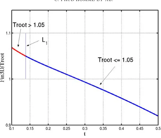
It is also now possible of course to find all values of Trootgreater than 1.05 fort in the range [0.1,0.5] and all other parameters fixed as in the list above. To wit, we enter
i=1;
while( i < 1000 )
p.values(6).value=0.1+i*(0.4)/1000;
Figure 4. Plot.
t(i)=p.values(6).value;
[o(i),e(i)] = fin3d_Troot( p ); i=i+1;
end
plot(x(o<1.05),o(o<1.05),’b’); hold on; grid on; plot(t(o>=1.05),o(o>=1.05),’r’);
line([max(t(o>1.05)) max(t(o>1.05))], [1 1.1]); %% L1
which generates Figure 4. Where the lineL1splits the domain [0.1; 0.5] attmax = max(t(o > 1.05)) = 0.1380 between the values of Trootgreater than 1.05 (t < tmax) and the values of Trootless then 1.05 (t ≥tmax). To be more certain that Trootwas trulygreater than 1.05, we could easily ask for those values oft for which
sN −∆N ≥1.05; again readily effected by a simple function call. Obviously, once the on-line code is within the MATLAB environment, we have the full functionality of MATLAB at our disposal; and the rapid response of the reduced–basis output bounds maintains the immediate response expected of an interactive environment, even though we are in fact solving — and solving reliably — three-dimensional partial differential equations.
5.4.
Overview of the framework
5.4.1. Introduction
The main current trend in computing and scientific computing is Distributed Objects — see for example the .NET, Mono, Globus, Netsolve, Seti@Home technologies and as mentioned earlier, we use Corba as the
underlying technology for our Framework.
Corba is the Distributed Objects technology developed and standardized by the OMG. As envisioned by Corba, Distributed Objects are the melding of concepts from two paradigms, Client-Server (or more precisely
Distributed Computing) and Object Orientation (OO) with some slight differences: (i) a Client knows an object by its interface; (ii) objects are not always local with respect to their Clients; (iii) dynamic composition may compose objects into new application; (iv) objects hide many of the underlying differences (between Client and Server) in architecture through encapsulation.
thanks to well-defined integration and interfaces. Another advantage is also that we can have much more complicated topologies — see, for example, Figure 3 — than typically found in the Client-Server paradigm: a Client request computation from a Server which is itself a composition of several other Servers; in this context, our requested object is a Client-Server — a Server for the Client and a Client for the Servers composing it.
It is interesting to note that although there is generally a many-to-one relation for Client to Server, Clients may want to have access to more than one Server for a given purpose. In the overview of our Framework we have seen that it was effectively the case (see Fig. 3). Indeed, if a single source can be beneficial, it can also be expensive: risk of central outage (single point failure), too little specialization (resource utilization is suboptimal) long queues for services and large distances over which products chip and so on.
Development costs may rise also: distribution introduces more difficult problems such as, for example, the logistics of coordinating multiple sites. Two other particularly serious issues are the network latency and the
scalability. They are difficult to determine beforehand and they can undermine gravely the deployment of the Framework.
Those issues are partly addressed by the numerical methods proposed (see Sect. 5.1). Only partly because the network latency is a difficult issue and reducing it is by no means easy — see the Akamai technology7. And regarding thescalability, the numerical methods proposed are not sufficient — although lots of problems (scheduling, monitoring, ...) arising when using more conventional methods are of no concern in the Reduced-Basis Output Bound methods context — therefore an adequate design for our Framework is also a requirement to ensurescalability.
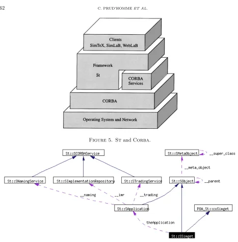
The Framework relies on a library,St8, which sits on top of CORBA (see Fig. 5) and its associated services.
Three Clients —SimTEX,SimLaB, WebLaB— have been developed withSt.
5.4.2. The main actors of St
The design of Stshares similar concepts to the one that can be found in modern Graphical User Interface
(GUI) libraries: the SApplication class and the SSimget class and their respective subclasses. Corba is
a complex middle-ware specification and through simple coarse grain interfaces and high level concepts St
encapsulates all Corba aspects — standard Corba calls or Corba Services — inside its classes. In the
following section, we shall describe briefly some aspects of the Framework.
SApplication.As shown in Figure 5, Stsits on top of Corba and the CorbaServices: it encapsulates all Corbaand associated components into a small set of classes with well defined behavior. Central to this design
is the St::SApplicationwhich encapsulates initialization of Corba, determines the available services and,
in Server mode usingSt::SApplicationServersubclass, drives the execution flow of the application through itsSt::SApplicationServer::run()method which is basically an infinite loop waiting for new requests from Clients, see Section 5.5.1. ASApplication, and subclasses, follows the Singleton pattern to ensure that there ex-ists only one instance of this class per process. It is possible to check for the availability on the Directory Service Server (see Fig. 3) of three standardCorbaServices through the member functionsbool hasNamingService(),
bool hasTradingService()andbool hasImplementationRepository()and have access to each to these Ser-vices through there associated class,SNamingService,STradingServiceandSImplementationRepository.
In practice, accessing the Corba Services directly from a Client or a Server is neither needed nor
recom-mended, it is usually taken care of by the objects that represent the Simulation objects, the Simgets.
An issue arising inevitably in Distributed Computing is Security. The most basic Security action that can be taken is related to the protection of the computers running the Servers: the processes associated to the Servers must have the lowest permissions on the system. On a Unix system for example, such a process would belong to the nobody user and group. By doing so, if someone with ill-intent manages to enter the operating system using those processes, he cannot do any harm. That is the least that has to be done. Unfortunately, ill-intended people can still do harm to the Framework. In order to avoid this, we use an authentication layer on top of the Framework using the Secure Sockets Layer (SSL). It has also the advantage to have some statistics on the
Figure 5. StandCorba.
Figure 6. The Simget collaboration diagram.
Framework usage. The inclusion of theMicoSecwhich is an implementation of theCorba Security Services
(CORBASec) Level 2 version 1.79 is underway. The current and future security features are/will be built-in SApplication.
SSimget.As described in the collaboration diagram (Fig. 6), a Simget is a SObject, base class for all St
objects, and also a Corba object through the interface POA St::coSimget. It contains a reference to the
reference of the SApplicationrunning in order to have access to the Corba Services to be able to register
itself automatically in each of them, provided that some of the Services are available. A Simget is a rather
complex object which is following the Composite pattern: it can be either a standalone computational object or a composite object of Simgets.
The constructor of the SSimgetclass and subclasses follows the prototype:
#include <SSimget.hpp>
SSimget( SSimget* parent, const char* name );
class A: public St::SSimget {
public:
A( St::SSimget* parent, const char* name ) : St::SSimget( parent, name )
{} };
whereparentis the parent Simget andnameis the name of the object passed toSObject— everySObjecthas a name. Then, using this composite or tree, it is possible to define a directory of Simgets in the variousCorba
Services. The name of the Simget and its relationship with the other ones will be used to define its location in the Services. For example, if the following code is executed:
St::SApplicationServer *app = new St::SApplicationServer; A * a = new A( 0, "a");
A * b = new A( a, "b"); A * c = new A( b, "c"); A * d = new A( a, "d"); app->setMainSimget( a );
then the Naming Service will contain the following references
console > nsadmin -ORBNamingAddr inet:<directory service computer>:<port of the service> > ls
a.a/ > ls a.a b.b/ d.d/
> ls a.a/b.b c.c/
nsadminis a tool provided by Micothat allows to browse the Naming Service using the UNIX-like tools like
lsorrm.
The SSimget is very general and is the base class for all Simgets. In the context of the Reduced-Basis methods and the Framework we built for them, we added other concepts which could be used to other kind of problems. First, we defined a model which is an object describing the model or problem being considered, for example Fin3D. The associated class is St::SModel. Then, we defined a model component which represents a general concept of model part. The associated class is SModelComponent. Finally, various subclasses of SModelComponentarise likeSModelOutput,SModelOutputSet, andSModelFieldwhich are associated with the computation respectively of one output and associated error estimation if available, of a set of different outputs and associated error estimations, or a field — say a Finite Element field associated with a Finite Element simulation. Each of these objects are CORBA objects and follow a relatively simple IDL10interface that allows their remote manipulation from a Client program. Here is the IDL interface for aSModelComponent
interface coModelComponent: coSimget {
//! get the name of the Model string getModelName();
//! set the new parameter set
void setParameterSet( in coParameterSeq pset );
//! set a new Range
void setRange( in coRangeSeq range ); };
andSModelComponentis defined as a subclass of SSimgetwhich implements the interfacecoModelComponent. The other classes,SModelOutput,SModelOutputandSModelField, have similar simple CORBA interfaces with further specification. For example aSModelComponentand subclasses have the following constructor
SModelComponent( SModel* parent, const char* name );
which means that a model component has to have a model as a parent Simget. The relationship model/component is enforced through this explicit constructor. For an implementation example see Section 5.5.1.
SMonitor.While monitoring is not an important issue for our Framework since we deal with black-box real-time response simulations, it is interesting however to collect statistics or to provide such a tool for future Simgets that will need monitoring. Monitors are Clients and Servers for the Framework, they are implemented using the Observer and Memento design pattern. The base class for monitors isSMonitor which encapsulates the commonalities for all monitors which are here the interfaces following the above-mentioned design patterns. The abstraction is that a Simget sends messages stored in a Memento upon special Events to the current Observers/monitors of the Simget. Monitors are Simgets which are Clients to the Simulation Simgets. Here is a short code snippet to describe how it works
St::SApplicationServer* app = new St::SApplicationServer;
St::SMonitorOutput* mon = new St::SMonitorOutput( 0, "monitor", SYSLOG );
mon->setMonitor( St::MONITOR_TIME | St::MONITOR_RESULT | St::MONITOR_PARAMETERS ); app->setMainSimget( mon );
app->run();
the second line creates a monitor for all Simgets in the Directory Services which will use syslog to log events like computation time, results from the Simgets and parameters passed to the Simgets. In order to create a model specific monitor for the Fin3D model and its outputs, we use the following code for example:
St::SApplicationServer* app = new St::SApplicationServer; St::SModel* model = new SModel( 0, "fin3d" );
St::SMonitorOutput* mon = new St::SMonitorOutput( fin3d, "monitor", SYSLOG ); mon->setMonitor( St::MONITOR_TIME | St::MONITOR_RESULT | St::MONITOR_PARAMETERS ); app->setMainSimget( model );
app->run();
A monitor can just log events but it provides also a CORBA interface that allows Clients like SimTEXfor example to access statistics of the Simget being called. Note that this Monitor design pattern is not only used byStto provide monitoring of the Simget but it is also used for all kind of objects that requires monitoring like
several design patterns and is a reusable component/strategy in scientific computing libraries. We just provided an application in the context of the Framework and Distributed Computing.
XML. XML11 is another trendy technology and it is often associated with Distributed Computing — see SOAP12 or XML-RPC13. The eXtended Markup Language is used in the Framework as a meta-data language to describe the Simgets. If it exists at the creation of a Simget, an associated XML file is loaded and is available through the CORBA interface of the Simget. In the current implementation, the XML data contain only static information like the name of the Simget, the model name, some parameter set data — like the name of the parameters, their minimum and maximum values, and a description — and a description of the Simget. Here is a simple XML example:
<!DOCTYPE St> <St>
<SModelOutput name="Troot" parent="fin3d" model="fin3d">
<Author firstname="Christophe" lastname="Prud’homme"></Author> <Basis db="fin3d_Troot.bb" N="20" Nused="20"></Basis>
<ParameterSet name="D" dimension="7">
<Parameter ub="10" lb=".1" name="k1">k1</Parameter> <Parameter ub="10" lb=".1" name="k2">k2</Parameter> <Parameter ub="10" lb=".1" name="k3">k3</Parameter> <Parameter ub="10" lb=".1" name="k4">k4</Parameter> <Parameter ub="1" lb=".01" name="Bi">Bi</Parameter> <Parameter ub="3" lb="2" name="L">L</Parameter> <Parameter ub=".5" lb=".1" name="t">t</Parameter> </ParameterSet>
<Description>
Troot computes the temperature at the root of the 3D Thermal Fin.
BlackBox: O(Q^2) in compliant case.
See http://augustine.mit.edu/fin3d_1/fin3d_1.pdf for more details. </Description>
</SModelOutput> </St>
This is particularly helpful for automatic generation of Clients for the Framework. For exampleSimLaBuses
this feature to automatically generate.mfiles for the Simgets registered in the Directory Service (see Sect. 5.3.2). Without having to communicate with the Server, the Client can for instance provide documentation about the Simget, and checks that the parameter set which will be sent to the Server is contained inD(see Sect. 3.1).
In the future an automatic C++code generator for the Clients will be implemented using the XML
meta-data provided by the Simgets registered in the Directory Service. At present onlySimLaBdoes automatic code
generation using the XML meta-data.
5.5.
A simple Client/Server implementation in C++
In a Client-Server paradigm, we have a Server side and a Client Side. In the next sections, we are going to present a sample code of a Server running the Simget computing the temperature at the root of the 3D thermal fin and one possible — while very simple — Client code in C++ accessing the code and the equivalent
in MatLaB using SimLaB in order to compare the amount of work needed. Some knowledge of C++ is
required, however some of the general ideas and concepts appear in the code.
5.5.1. Server side
First look at what the main program looks like from the server point of view:
#include <SApplicationServer.hpp> using namespace St;
int main(int argc, char** argv) {
SCommandLineArguments::init( argc, argv );
SApplicationServer* server = new SApplicationServer();
server->run(); }
The line 6 initializes the command line parsing system. Then, we define the St Server application using
the SApplicationServer class. Unfortunately this example does nothing but running forever. Indeed the server->run()is an infinite loop, where the serveris waiting for new requests.
Now we need to feed the server with Simgets.
SApplicationServer* server = new SApplicationServer(); SModel* fin3d = new SModel( 0, "fin3d");
server->setMainSimget( fin3d ); server->run();
With the two new lines 2 and 3, we have created a possibly new Model in the St Services (Naming and
Trading). First we define the "fin3d" model — second argument — which has no parent in the current SApplicationServer — first argument. Again this server is not very helpful, since it does not do any real computation.
We can add for example a Simget which compute the temperature at the root of the three-dimensional thermal fin — see line2in the next listing.
SModel* fin3d = new SModel( 0, "fin3d");
SModelOutput* troot = new Troot( fin3d, "Troot"); server->setMainSimget( fin3d );
The work in the main program is finished and doesn’t need further work. whenserver->run()is executed the server will provide the TrootSimget associated with the modelfin3d.
Now let us see what theTrootlooks like:
#include <SModelOutput.hpp> using namespace St;
class Troot: public SModelOutput {
public:
Troot( SModel* parent, const char* name ): SModelOutput( parent, name ) {<snip> } virtual SOutput* run( SParameterSet const& pset )
{
SOutput* output = new SOutput;
. . .
output->output = <prediction value>;
output->error = <associated error estimator value>; return output;
} };
The last step is the execution of the Server:
fin3d_Troot --server augustine.mit.edu --daemon
The--serveroption tells the SApplicationServerto register the Simgets in augustine.mit.edu. Whereas the--daemontellsSApplicationServerto detach from its parent process and run forever in the background. Under Unix/Linux, a database and theinit.dsystem are used to start and stop automatically the Servers used and registered on one computer. The advantage is that if a computer containing Simgets is rebooted or shutdown for some reason then the Simgets will be cleanly shutdown. Indeed, one of the major difficulty with Distributed Computing is the fact that the Object haveexternal references and they need to be deleted properly if the corresponding is being shutdown.
Looking back at the example presented above, it would seem that it is possible to have only one Simget per process. Recall the tree structure of the SObject/Simget classes plugged into SApplicationServerusing its setMainSimget()member function, then enabling new Simgets in the same process as the one presented earlier is a one-liner per Simget provided that each Simget has been implemented likeTrootfor example.
SModel* fin3d = new SModel( 0, "fin3d");
SModelOutput* troot = new Troot( fin3d, "Troot"); SModelOutput* ttip = new Troot( fin3d, "Ttip"); SModelOutput* volume = new Troot( fin3d, "Volume"); server->setMainSimget( fin3d );
The code shown above adds two Simgets to the Framework — in this case the temperature at the tip of the 3D fin and the volume of the 3D fin. As one can see, in one process we can register one or more components for a given Model in the various services available and the associated code and programming time are reduced.
A note on parallelism.Finally let us present a possible extension for the Server part: the various registered Simgets in one process are often independent from each other — eventually a Simget could depend on the computation done by another one. For example a Simget providing a dimensionalTrootwould depend on the non-dimensionalTrootcounterpart: this kind of dependency requires generally simple algebra while the non-dimensionalTrootwould require an Online Code as described in Sections 3 and 4. The Simget could be accessed by several users at the same time, and it appears that exploiting parallelism is important in this case to make sure that the Framework is responsive enough with respect to multiple Clients and provide Real-Time response for each Client. We implement parallelism at two levels on the Server side. Firstly, we use a multi-threaded CORBA implementation — MICO/MT14which is about to be or already merged with MICO15— that enables us to answer “simultaneously” to concurrent requests. Secondly, we implement thread-safe Simgets so that when the Client asks for multiple evaluations — say a thousand randomly chosen parameters — we use the interface of SModelOutputwhich provides multiple parallel evaluations — seeSModelOutput::run(MultiParameter)in the next section. In order to control the level of parallelism for many outputs, the SApplicationbase class provides a way of defining the number of possible multiple threads.
SApplicationServer* __app = new SApplicationServer;
// tell thread-aware classes (SModelOutput for example) // and their subclasses to use up to 3 threads for // many outputs evaluations
__app->setNumberOfProcessors( 3 );
The Framework provides a simple way to allow multi-threaded classes. The developer has to use the class SThreadas the base class for a multi-thread enabled class. Here is an example:
#include <iostream> #include <SThread.hpp>
class A: public St::SThread {
public:
// a possible default constructor
A( int __no = 1 ): St::SThread(), _M_no( __no ) {}
protected:
// run() method has to be re-implemented void run()
{
St::SMutex __mutex; if ( __mutex.tryLock() )
{
std::cerr << "run thread number " << _M_no << std::endl; }
else {
;//locking did not work }
// __mutex.unlock() is called by destructor automatically // so no need to call it here
} private:
int _M_no; };
Note the utilization of the mutex class SMutex — which is provided by SThread.hpp — to ensure that the output will be written sequentially in the console instead of having both threads outputs being mixed up. Then the controller program can do the following:
int main( int argc, char** argv ) {
St::SCommandLineArguments::init( argc, argv ); St::SApplication* __app = new St::SApplication; // can either use NPROCS environment variable or
// SApplication::setNumberOfProcessors( n ) to set the number of threads int __nprocs = __app->getNumberOfProcessors();
A** __threads = new A*[ __nprocs ]; for( int __i = 0; __i < __nprocs; ++__i )
// start a new thread and call thread1.run() __threads[ __i ] = new A( __i );
__threads[ __i ]->start(); }
// wait for all threads to finish
for( int __i = 0; __i < __nprocs; ++__i ) {
__threads[ __i ]->wait(); }
}
The environment variable NPROCS controls the number of threads than can be used, it is overridden by the SApplication::setNumberOfProcessors( int )member function. When running the above code, we get the following expected console output:
console > export NPROCS=4 console > test_thread run thread number 0 run thread number 1 run thread number 2 run thread number 3
The various classes handling the Online Codes computation usesSThreadwhich eases the use of multi-thread programming by encapsulating all the pthreadlibrary.
To summarize, parallelism is achieved at two levels on the Server side: at the ORB level using a multi-threaded ORB and at the Simget level. Note that it is transparent to the Framework user except for the part he has to provide the number of threads and that his code has to be thread-safe in order to be used in this multiple threads (>1) environment. If it is not thread-safe then the Framework user can still fall back to a single thread environment which is the default and conservative behavior. There is a Client parallel counterpart which is discussed in the next section which uses yet another feature of the Framework.
5.5.2. Client side
On the client side, the Client developer has access to the Naming and Trading services in order to find the object he is looking for. In the next listing, we present a client using the Naming service. The way the Simget in general are stored in the Naming service resembles a directory tree where/is the root of the tree. Under the fin3dmodel appears the Troot,TtipandVolume Simgets. In the following example, we retrieve a reference to theTrootSimget and use its interface to do some computations:
#include <SApplication.hpp> #include <SModelOutput.hpp> using namespace St;
int main(int argc, char** argv) {
SCommandLineArguments::init( argc, argv ); SApplication* client = new SApplication();
SModelOutput_var fin3d_troot = client->resolve( "fin3d/Troot" ); fin3d_Troot->setNewParameterSet( pset );
fin3d_troot->run( MultiParameter );
coOutputArray_var results = fin3d_Troot->getOutputs(); for( ULong __i = 0;__i < __output_pl->length();++__i)
{
std::cerr << "output( " << __i << ")=" << result( __i ).output << std::endl; std::cerr << "error( " << __i << ")=" << result( __i ).error << std::endl; }
}
The onlynon standardC++ statement is the call toclient->resolve()which will lookup in the naming service in order to get an handle on the corresponding simulation which was defined earlier. The other statements are classical object manipulation, setting the parameter set, set the range if needed, run the simulation and then retrieve the results.
Writing a client for the framework is relatively easy task, however providing a graphical user interface to the client code certainly comes with some efforts, that one of the reason why we based SimTEXandSimLaB
Clients upon existing standards(MatLaBandPDF) — to alleviate the work in programming user interfaces.
Now it remains to execute the Client program:
fin3d_Troot_client --server augustine.mit.edu
This command line tells the Client to contactaugustine.mit.edufor Simget lookups.
A note on parallelism.Parallelism is/can be also implemented on the Client side. However it is not an automatic builtin feature of the Client. The Framework allows to implement a Client which takes advantage of certain of its properties. The starting point is that, as mentioned in the previous section, the ORB is multi-threaded and recall that several instances of the same Model/Simget can exist in the CORBA Services — namely the Naming or the Trading Services — so with those two features one can build a Client which access several instances of the same Simget or several different Simgets at the same time in different threads. TheSThreadclass presented in Section 5.5.1 can be used to implement such a multi-threaded Client. Another important part here is the load balancing system of the Services which ensures that the least used instance will be selected by the Service to answer each new request.
To summarize the parallelism aspects of the Framework, both Server and Client sides, we achieved a three levels parallelism which ensures real-time response — with the certificates of fidelity developed in the first sections of the paper — in the context of many evaluations and many users.
6.
Conclusion
This framework is likely to be extended in the next few months, and will certainly enjoy some improvements. It has already been tested on many problems already available online on our web site http://augustine.mit.edu. The component-wise design of the overall system is very flexible, scales well as the number of Online Codes increases and is an elegant solution as a platform for engineering design, research and education. Regarding the mathematical framework, it has been extended to several problem categories: non-coercive partial differential equations, parabolic equations, generalized eigenvalue problems, non-symmetric and non-compliant cases, see [19].