Quantifying Regional-Scale Water Storage Using Models and Observations: Application For Drought Assessment In South Carolina

(1)

University of South Carolina

Scholar Commons

Theses and Dissertations

1-1-2013

Quantifying Regional-Scale Water Storage Using

Models and Observations: Application For

Drought Assessment In South Carolina

Mirza Md Mozaddid Billah

University of South Carolina

Follow this and additional works at:https://scholarcommons.sc.edu/etd Part of theCivil and Environmental Engineering Commons

This Open Access Dissertation is brought to you by Scholar Commons. It has been accepted for inclusion in Theses and Dissertations by an authorized administrator of Scholar Commons. For more information, please [email protected].

Recommended Citation

(2)

Quantifying regional-scale water storage using models and observations: Application for drought assessment in South Carolina

by

Mirza Md Mozaddid Billah

Bachelor of Science

Bangladesh University of Engineering and Technology, 2003

Master of Science

UNESCO-IHE Institute for Water Eduction, 2007

Submitted in Partial Fulfillment of the Requirements For the Degree of Doctor of Philosophy in

Civil Engineering

College of Engineering and Computing University of South Carolina

2013

Accepted by:

Jonathan L. Goodall, Major Professor Michael E. Meadows, Committee Member

Venkat Lakshmi, Committee Member Enrica Viparelli, Committee Member

(3)

c

(4)

Dedication

(5)

Acknowledgments

My deepest gratitude is to my advisor, Dr. Jonathan Goodall. I have been amazingly fortunate to have an advisor who gave me the freedom to explore on my own, and at the same time the guidance to recover when my steps faltered. I am also thank-ful to him for encouraging the use of correct grammar and consistent notation in my writings, and for carefully reading and commenting on countless revisions of this dissertation. Dr. Michael Meadows’ insightful comments and constructive criticisms at different stages of my research were thought-provoking and they helped me focus my ideas. Dr. Venkat Lakshmi has always been there to listen and give advice to overcome crisis situations. I am deeply grateful to him for his continuous encourage-ment and guidance. I am grateful to Dr. Enrica Viparelli for her encourageencourage-ment and practical advice. I am also thankful to her for reading my reports, commenting on my views and helping me understand and enrich my ideas. I am grateful for the support by the National Science Foundation under the grant NSF ACI 0940841 “DataNet Full Proposal: DataNet Federation Consortium’’ for completing my dissertation.

(6)

Abstract

Hydrologic models are widely used to determine the occurrence and severity of droughts, and to aid in the decision making process for reducing drought impacts. These models apply approaches including water and energy balance equations to determine water availability at field to continental scales. One challenge in implementing hydrologic models at regional to continental scales is the lack of data with sufficient spatial and temporal resolution to represent actual conditions within the study domain. If such data are available, the challenge remains how best to find, access, and process the information contained within the datasets so that it can be used within hydro-logic models. The overarching goal of this work is related to both these data-related challenges of modeling regional-scale hydrologic systems, as well as to the hydrologic science challenges of quantifying water storage within regional-scale hydrologic sys-tems. Three research studies are presented that address specific challenges as they relate to estimating high resolution, large-scale water storage and drought severity at seasonal and interannual scales in South Carolina.

(7)

storage decreases due to drought conditions and, more importantly, the complexity of the spatial patterns in drought impacts across the state.

The second study builds on the first study by quantifying the accuracy of es-timates of evapotranspiration across the state. Two methods for estimating evapo-transpiration at regional scales are investigated as part of the work: simulation of evapotranspiration using the Variable Infiltration Capacity (VIC) macro-scale hy-drologic model and remote sensing of evapotranspiration using Moderate Resolution Imaging Spectroradiometer (MODIS) derived estimates. The results of this analysis show that, when VIC-derived evapotranspiration are applied within a water balance framework, estimates of changes in water storage match better with estimates of water storage from the Gravity Recovery and Climate Experiment (GRACE) Ter-restrial Water Storage (TWS) anomalies product. Therefore it was concluded that VIC-derived estimates of evapotranspiration were nearer the true values of evapo-transpiration for the study area and period of analysis.

(8)

(9)

List of Tables

Table 3.1 Summary of geospatial and hydrologic time series data used in

the study. . . 28 Table 3.2 Annual rate of change in terrestrial water storage (m3 _s−1_{) for}

all sub-watersheds. . . 33 Table 3.3 Seasonal rate of change in terrestrial water storage (m3 s−1) for

all sub-watersheds. . . 34

Table 4.1 Description of the parameters used in the VIC model calibration. . 55 Table 4.2 Groundwater monitoring wells used for evaluating water storage

estimates. Depth to water level values are given as an average (±1s.d.) of monthly observations during the study period (2000

- 2007). . . 58 Table 4.3 Correlation coefficients between monthly average depth to

groun-dwater level and cumulative water storage estimates based on VIC and MODIS derived ET estimates. Results for all sub-watersheds in the study region are given in the SC column. The PD, CW, BS, and SV columns provide results for sub-watersheds in the Pee Dee, Catawba, Broad/Saluda, and Savannah River

Basins, respectively. . . 65

Table 5.1 List of micro-services applied for VIC model application using

(12)

List of Figures

Figure 2.1 Locations of the monitor wells, lakes levels and stream gages

used for drought study (from Gellici et al., 2004). . . 7 Figure 2.2 Temporal variation of groundwater level at Well CHN-14 during

the period of drought from 1998-2002 (from Gellici et al., 2004). . 8 Figure 2.3 Temporal variation of lake level at Lake Jocassee during the

period of drought from 1998-2002 (from Gellici et al., 2004). . . . 9 Figure 2.4 Temporal variation of streamflow at Little Pee-Dee River at

Galivants Ferry (Station 02135000) during the period of drought

from 1998-2002 (from Gellici et al., 2004). . . 10

Figure 3.1 Map of the study area showing gaged sub-watersheds, aquifers (a) Piedmont and Blue Ridge aquifers (b) Southeastern Coastal

Plain aquifers (c) Surficial aquifers . . . 23 Figure 3.2 Annual variations (box with 25th, 50th, and 75th percentiles,

whiskers with minimum and maximum values, and outliers ob-servations as “+" marks) of precipitation, evaporation,

stream-flow and ∆T W S/∆t in the sub-watersheds. . . 30 Figure 3.3 Seasonal variations (box with 25th_{, 50}th_{, and 75}th _percentiles,

whiskers with minimum and maximum values) of precipitation, evaporation, streamflow and ∆T W S/∆tin the sub-watersheds) of precipitation, evaporation, streamflow and ∆T W S/∆tin the

sub-watersheds. . . 31 Figure 3.4 Spatial variation of rate of change in terrestrial water storage

in the sub-watersheds. . . 36 Figure 3.5 Location of the focus sub-watersheds in South Carolina. . . 38 Figure 3.6 Relationship between cumulative rate of change in cumulative

terrestrial water storage (averaged over same month from

1998-2007) and groundwater levels (1998-1998-2007) in the sub-watersheds. . 39 Figure 3.7 Long term relationship between the yearly cumulative rate of

(13)

the sub-watersheds. . . 41

Figure 4.1 The study area including the sub-watersheds for which change in storage has been estimated grouped into four major river basins (Pee Dee, Catawba, Broad/Saluda, and Savannah). Also shown are the locations of groundwater wells used for model

evaluation. . . 48 Figure 4.2 Monthly precipitation and streamflow averaged for (a) all

sub-watersheds in the study area and (b-e) for the four major river basins in the study area. Streamflow and precipitation have been normalized by sub-watershed area and therefore are

ex-pressed in length units. . . 50 Figure 4.3 (a) Calibration of the VIC soil moisture with SCAN soil

mois-ture observations at the Savannah site and (b) validation of the VIC soil moisture with SCAN soil moisture observations at the

Pee Dee site. . . 53 Figure 4.4 Streamflow comparison between VIC model predictions and

USGS observations. The comparison is performed at the USGS station Little Pee Dee River at Galivants Ferry, SC (Station Number 02135000) and Broad River at Carlisle (Station

Num-ber 02156500). . . 56 Figure 4.5 Monthly average ET from NARR, VIC, and MODIS averaged

for (a) all sub-watersheds in the study area and (b-e) for the four major river basins in the study area. ET has been normalized

by sub-watershed area and therefore is expressed in length units. . 60 Figure 4.6 Cumulative change in storage over the study period using

evap-otranspiration estimates from VIC and MODIS, and GRACE for (a) all sub-watersheds in the study area and (b-e) for the

four major river basins in the study area. . . 62 Figure 4.7 Annual cumulative change in storage for each year of the study

period generated using estimates evapotranspiration estimates from VIC and MODIS estimates and the difference between the

two estimates. . . 64 Figure 4.8 Comparison of cumulative change in water storage using

evapo-transpiration estimates from VIC and MODIS for the Broad/Saluda River basin (primary axis) with depth to groundwater

(14)

Figure 5.1 Data pre-processing steps for VIC model (adopted from Gao

et al., 2010). . . 73 Figure 5.2 Schematic diagram of the NSF supported Data Federation

Con-sortium (DFC) data management system showing the

connec-tions between DFC-Hydrology with DFC-Federation Hub. . . 76 Figure 5.3 Model pre-processing workflows showing the major steps for

transforming datasets to set up a VIC model for a specific study area. Rules are initiated from a client but executed on a server

using micro-services. . . 80 Figure 5.4 Data flow in the hydro1kCarolinas.r rule that extracts climate

data from NCDC GHCND using HYDRO1k basin/DEM datasets

to define a study region. . . 82 Figure 5.5 Study area with major river basins in North and South

Car-olina, USA. These subwatersheds were extracted using selected Pfafstetter Basin Code from the Hydro1K dataset. The sub-watershed and stream gage station used for VIC model

calibra-tion is also shown in the Figure. . . 84 Figure 5.6 Streamflow comparison between VIC model predictions and

USGS observations. The comparison is performed at the USGS station Little Pee Dee River at Galivants Ferry, SC (Station

Number 02135000). . . 85 Figure 5.7 Comparison of monthly averaged soil moisture in the three soil

layers predicted by VIC model in the Carolinas for the periods

(15)

Chapter 1 Introduction

Extreme weather and climate events can have deep impacts on the environment of the affected regions (Ruiz-Barradas and Nigam, 2006b). Events such as the severe drought in South Carolina during the period 1998-2002 support this claim. This drought event, caused by decreased precipitation of 10-30% from normal levels, re-sulted in reduced groundwater levels, lake levels, and streamflow across the state (Badr et al., 2004; Gellici et al., 2004). The drought presented challenges in meeting the water supply demands for domestic and industrial purposes, and also intensified water right issues on the rivers shared with neighboring states (Sabo et al., 2010). Projected population increases and increased uncertainty of future weather conditions due to climate change will only intensify problems caused by future drought condi-tions, making timely determination and decision making during times of drought very important in reducing negative impacts.

(16)

to regional scales (Gerten et al., 2004; Yang et al., 2008; Wang et al., 2009). At an increased level of sophistication and complication, hydrologic models can be used to simulate mechanistic processes including soil and vegetation dynamics to understand non-linear hydrologic system responses (Meselhe et al., 2009), and these simulations can be applied to large-scale basins across the globe (Liang et al., 1994, 1996; Lak-shmi et al., 2004; Troy et al., 2008). Beyond these approaches, another powerful tool available to hydrologists is satellite remote observation of hydrologic conditions. An example of this is the Gravity Recovery and Climate Experiment (GRACE) product that provides a means of monitoring changes in the terrestrial water storage at re-gional to global scales (Swenson et al., 2003; Rodell et al., 2004, 2007; Landerer and Swenson, 2012).

(17)

aims at conducting studies that make use of all three approaches to gain a more complete picture of water storage in South Carolina.

In the first study, a water balance model is used for quantifying water storage for regions in South Carolina for the period of 1998-2007. The specific water bal-ance approach used builds from the Precipitation, Evapotranspiration and Runoff (PER) approach (Zeng et al., 2008) and is applied to estimate water storage in terms of rate of change of terrestrial water storage. The study area is divided into 54 sub-watersheds defined by the drainage area between consecutive streamflow gaging stations and derived using flowline and catchment feature classes from the National Hydrography Dataset (NHD) and the NHDPlus program, along with terrain pro-cessing algorithms that were operated on the National Elevation Dataset (NED). In each of these sub-watersheds, observed precipitation from Parameter-Elevation Re-gressions on Independent Slopes Model (PRISM) Group, observed streamflow from United States Geological Survey (USGS), and estimated evapotranspiration from North American Regional Reanalysis (NARR) program are combined on a monthly time step to estimate changes in water storage as a function of time. This quan-tification of water storage is then compared to observed groundwater levels and this comparison shows evidence of annual and interannual variations as well as drought impact. The correlation of water storage estimates with observed groundwater level provides evidence of the level of connectivity between surface and subsurface water for different regions of the state.

(18)

de-gree and the second approach uses a Moderate Resolution Imaging Spectroradiometer (MODIS) derived approach for estimating evapotranspiration with spatial resolution of 1 km. Both evapotranspiration estimates are synthesized with observed precipi-tation and streamflow within the water balance approach for the sub-watersheds in the study region. In this second study, a water balance calculation is applied to 44 sub-watersheds derived using a methodology that improved on the methodology used in the first study. The estimated water storage using two different evapotranspiration are evaluated with independent observations of GRACE TWS anomalies product and groundwater levels observations.

The third and final study investigates the application of novel cyberinfrastructure to improve on the methodology for constructing, sharing, validating, and documenting a sophisticated hydrologic simulation model such as VIC. VIC, like other hydrologic simulation models, requires a significant amount of time and resources to collect and process the data required to parameterize, calibrate, and evaluate the model. To address this challenge, the sequence of steps required to create the input files for VIC were implemented into automated workflows using the Integrated Rule-Oriented Data System (iRODS). The automated workflows executed both the data preparation steps as well as the post-processing steps required to create visualizations and analyzes of drought conditions from the model outputs. The work advances on a goal within the hydrologic community to create community hydrologic models by providing a means for sharing model inputs, processing routines, model codes, and model outputs using a state-of-the-art data management system.

(19)

(20)

Chapter 2 Background

This chapter first presents background on the 1998-2002 drought experienced in South Carolina, followed by background on the water balance framework used to estimate water storage for sub-watershed in South Carolina. Next a brief overview on the importance of reliable input datasets for regional-scale watershed modeling is pre-sented, with an emphasis on evapotranspiration. The application of the VIC model for estimating evapotranspiration is discussed, followed by a discussion on the use of MODIS remote sensing imagery for estimating evapotranspiration. Finally, back-ground on Integrated Rule-Oriented Data System and its application to automate the procedures of collection and processing sourced datasets, curation, preservation, and replication of the large amount of processed datasets for VIC model are presented.

2.1 The Impact of the 1998-2002 Drought on South

Car-olina Water Resources

(21)

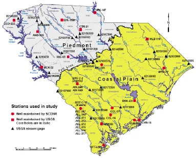
ground-water table depth, lake level, and streamflow stations throughout the state (Figure 2.1).

Figure 2.1: Locations of the monitor wells, lakes levels and stream gages used for drought study (from Gellici et al., 2004).

(22)

in groundwater levels during the period of drought. Wells in the Piedmont aquifers showed an annual decrease between 0.4 and 1.9 feet, while wells in the central part of the state in Southeastern Coastal Plain aquifers showed the decrease between 0.5 to 1.1 feet. Wells in the Surficial aquifers showed the highest annual decrease with a large variation ranging between 0.3 to 8.9 feet. The lowest water level was monitored in the Well CHN-14 in the Surficial aquifers with a decrease of 44.5 ft during the period of drought (Figure 2.2).

Figure 2.2: Temporal variation of groundwater level at Well CHN-14 during the period of drought from 1998-2002 (from Gellici et al., 2004).

(23)

aquifers (Lake Marion and Lake Moultrie) decreased to 5.0 feet below operating levels (Gellici and Badr, 2004).

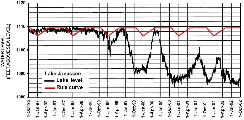
Figure 2.3: Temporal variation of lake level at Lake Jocassee during the period of drought from 1998-2002 (from Gellici et al., 2004).

(24)

at the Galivants Ferry monitoring station, located on the Little Pee Dee River, was at historical lows during the drought event (Figure 2.4).

Figure 2.4: Temporal variation of streamflow at Little Pee Dee River at Galivants Ferry (Station 02135000) during the period of drought from 1998-2002 (from Gellici et al., 2004).

2.2 Water Balance Framework

(25)

below the soil surface are considered as part of the terrestrial water storage (TWS) term. It is very important to apply appropriate approaches to measure TWS and its individual components for sustainable water management at the basin-scale.

(26)

small basins due to the fact that spatial extent may introduce error to the estimates (Swenson et al., 2003).

While the PER approach has been shown to be a robust approach for in estimat-ing water storage at different scales, the accuracy of the approach depends on access to the sufficiently high resolution input datasets. Although the observed datasets of streamflow and precipitation are considered reliable, estimates of evaporation at a regional scale remains a challenge. As will be shown in the study presented in Chapter 3, the large decreases in water storage estimates using PER approach in the study region are most likely due to over estimation of evapotranspiration by the NARR product. This study also provided evidence that, even if the NARR product is adjusted using a correction factor that ensures no net change in water storage over the period of study, the NARR evapotranspiration estimates do not capture local variability across the state due to the spatial resolution of the dataset. Therefore, this study concluded that there is a need for improved estimates of evapotranspiration for quantifying water storage accurately.

2.3 Evapotranspiration

(27)

data. In the second approach, MODIS satellite data is used as an alternative means for measuring regional-scale evapotranspiration.

As a semi-distributed, macro-scale hydrological model, VIC simulates complex interactions of water, energy, and vegetation using soil properties and meteorological forcing for a grid-based discretization of the land surface (Liang et al., 1994, 1996). The sub-grid variability of the land surface vegetation classes and soil moisture storage capacity are captured by using statistical operations (Gao et al., 2010). The nonlinear vertical movement of soil moisture from the lower soil zone to base flow captures interannual soil moisture behaviors, while top and mid soil moisture responds to daily and seasonal variations. VIC has been successfully applied to model a number of large river basins in United States (Abdulla et al., 1996; Wood et al., 1997; Shi et al., 2008) and has been shown to accurately simulate and forecast streamflow and other hydrologic variables at the river basin scale (Wood et al., 2002, 2005; Wood and Lettenmaier, 2006). Therefore, VIC was selected as a viable tool for estimating regional-scale evapotranspiration for the study region.

(28)

evapotranspiration using the Penman-Monteith equation (Monteith, 1965). A com-parison between the two methods showed that the Mu et al. (2007) methodology generates evapotranspiration with higher accuracy (Gao and Long, 2008; Timmer-mans et al., 2007).

Both evapotranspiration estimates, VIC and MODIS, were evaluated in terms of how well they were able to close the water budget for the study area. The application of the VIC model is a time, data, and resource intensive operation. Applying the model requires the collection of large amount of data from heterogeneous external sources as well as processing of these datasets before they can be used in a VIC model. The data preparation steps consume a significant amount of storage and computational capacity. Moreover, the need for human intervention to implement this workflow introduces a potential source of error and delays to the process. Therefore, overcoming these technical challenges that limit the application of models such as VIC for water resource management is an important problem facing the hydrologic community.

2.4 Data Management Cyberinfrastructure

(29)

potential to transform how we construct, share, and document hydrologic simula-tion models. Therefore, appropriate workflow and data management infrastructure is gaining interest in the geosciences and engineering for large model execution and data curation.

The Integrated Rule-Oriented Data System (iRODS) is a data grid cyberinfras-tructure system that facilitates policy-driven workflow management in a grid envi-ronment (Weise et al., 2008). The iRODS (Moore et al., 2009) is an open source cyberinfrastructure, developed by the Data Intensive Cyber Environments (DICE) group as the successor to the Storage Resource Broker (SRB) (JaJa, 2005) with sig-nificantly enhanced functionality. The enhanced functionality offers automatic access to heterogeneous external sources and large scale data analysis. The iRODS sepa-rates itself from the SRB using policies as rules that automate the process of data management within a data grid (Weise et al., 2008).

(30)

(31)

Chapter 3 Annual and interannual variations in

terrestrial water storage during and

following a period of drought in South

Carolina, USA

1

3.1 Abstract

The goal of this research is to quantify variations in both space and time of water stored in the terrestrial environment within South Carolina during and following a period of drought. We use a water balance approach that synthesizes observed and modeled hydrologic fluxes for sub-watersheds defined by the drainage area between streamflow gaging stations. We apply the approach for the period 1998-2007 to study the impact of a drought that occurred during the early part of this time period on terrestrial water storage within the state. Results from the analysis provide evidence of distinct annual and interannual variation in water storage for different regions of the state, with the fall season having a water surplus and spring season exhibiting a water deficit. The impact of the drought varied for different regions of the state depending in part on hydrogeological conditions including soil type and depth to the groundwater level. Comparing estimates of rate of change in terrestrial water stor-age with observed groundwater levels, as an independent validation of the terrestrial

(32)

water storage estimations, shows that many of the sub-watersheds within the state exhibited similar patterns between variation of rate of change in terrestrial water storage estimates and observed groundwater levels during the period of analysis, as expected. However, some sub-watersheds did not follow general annual and inter-annual variations in groundwater level or in estimated rate of change in terrestrial water storage relative to neighboring sub-watersheds. We speculate that these ab-normalities may be related to human influences that alter local water storage trends within specific sub-watersheds of the state, however future work is needed to further investigate this possible explanation. We conclude through this study that the water balance approach presented is a simple yet valuable means for estimating variations in water availability at a regional spatial scale by synthesizing existing observations and model output data within a geospatially-explicit context.

3.2 Introduction

(33)

un-derstanding regional water resources under a variety of demands and stresses. We present research that investigates an approach for quantifying regional scale water balances through an application case study for river basins whose rivers flow through South Carolina.

Hydrologic modeling and analysis can aid in this problem by providing esti-mates of future water availability under changing conditions such as climate change, land use change, and increasing water demands (e.g., Lettenmaier et al., 1999; Rossi et al., 2008; Tung and Haith, 1995; Legesse et al., 2003; Wurbs et al., 2005). De-tailed, physically-based models of regional-scale hydrologic systems used to address such questions can be problematic for reasons that have been well described in the literature (e.g., Grayson et al., 1992; Jakeman and Hornberger, 1993; Beven, 2002; McDonnell et al., 2007). Part of the problem has been that, at the river-basin-scale, hydrology is subject to complex interactions between physical, biological, and so-cial systems, and no model is capable of addressing all of the interactions at play in watershed systems. Furthermore, those models that do attempt to simulate such interactions are difficult to parameterize and calibrate at a regional scale due in part to a lack of data describing system parameters, initial conditions, and boundary con-ditions. This leads to the need for uncertainty analysis both in terms of process representations, system parameters, and forcing data (Minville et al., 2008; Yang et al., 2008; Fekete et al., 2004; Christensen and Lettenmaier, 2007).

(34)

Moisture Convergence minus Runoff (MCR) approach (Rasmusson, 1967; Senevi-ratne et al., 2004; Yeh et al., 1998). In this approach, water balance equations for the terrestrial and atmospheric portions of the hydrologic cycle are equated to es-timate the rate of change in terrestrial water storage (TWS). TWS is a term that includes all stores of water within the terrestrial environment including soil mois-ture, snow, groundwater, and surface water. The MCR approach has been applied to river basins within Europe, Asia, North America, and Australia (Hirschi et al., 2006, 2007), demonstrating that the MCR approach can successfully estimate TWS on a monthly time step after comparing estimates with independent measures of TWS including soil moisture, groundwater levels, and snow depths. More recent work by Zeng et al. (2008) proposed a modification to the MCR approach where, instead of equating water balance equations for the surface and atmospheric systems, the surface water balance equation is solved directly by using observations of precipitation and stream discharge along with estimates of evaporation derived from climate reanalysis to quantify changes in TWS. This approach, termed the Precipitation, Evapotran-spiration, and Runoff (PER) method, was shown to be more robust in estimating TWS for the Amazon Basin and the Mississippi Basin when compared to the MCR approach and validated against independent estimations of TWS components (Zeng et al., 2008). Details of the PER method and how it compares to the more commonly used MCR method are provided in the Methodology Section of this paper.

(35)

(Fer-guson et al., 2010), and it is uncertain if remote sensing observations of evaporation will be effective at closing the water balance (Sheffield et al., 2009). Future research would be required to address the benefit of remote sensing derived evapotranspira-tion estimates compared to NARR evaporaevapotranspira-tion estimates. Despite the uncertainty of evapotranspiration estimates, a comparative analysis of the estimated evapotranspi-ration from different climate model and reanalysis datasets (ERA40, NCEP2, NARR, and SLand) in the PER model suggested that evapotranspiration estimates have a small variation relative to difference between observed precipitation and streamflow, therefore capturing variation in precipitation and streamflow is most important for estimating the rate of change in TWS (Zeng et al., 2008).

In this paper we use the PER method with NARR estimates of evapotranspira-tion to understand how water resources within South Carolina responded during and following the 1998-2002 period of drought. Using observational data from stream-flow and precipitation monitoring networks along with estimations of evaporation from climate model reanalysis products, we estimated rate of change in TWS on a monthly time step for 54 sub-watersheds where stream inflow and outflow were mon-itored for the period 1998-2007. The sub-watersheds were defined using geospatial data describing the terrain, hydrography, and streamflow gaging network and account for 60% of the surface area within the state. We then compared estimates of rate of change in TWS obtained using the PER method with groundwater levels in the state to determine how both measures of water storage varied during and following the period of drought.

(36)

better than 1 cm of equivalent water thickness with spatial extent of 4.0×105 _km2

or larger, and these accuracies increase with the increase in the spatial extent. Given that the total area of South Carolina is one-fourth the recommended area for ap-plication of GRACE data, we could not justify the use of GRACE as a means for validating our analysis estimates of change in TWS.

Following a brief description of the study area, we next describe our methodology for the study including a more detailed description of (1) the water balance method on which this analysis is based, focusing in particular on how the PER method compares to the more common MCR method for estimating rate of change in TWS and (2) the datasets and data preparation steps carried out as a part of the analysis. We next discuss the resulting estimates of the rate of change in TWS for the state summarized in space and time, including a comparison between rate of change in TWS estimates and observed groundwater levels. Finally we conclude with a discussion of the benefits and weaknesses of the PER approach for estimating rate of change in TWS, and suggest future directions needed to improve the approach as a tool for regional-scale water resources management.

3.3 Study Area

South Carolina is located in the Southeastern United States and has an area of 82,930 km2 _{(32,020 mi}2_{) from latitude 32}◦₀₂0_N _{to 35}◦₁₃0_N _{and longitude 78}◦₃₂0_W

(37)

aver-Figure 3.1: Map of the study area showing gaged sub-watersheds, aquifers (a) Pied-mont and Blue Ridge aquifers (b) Southeastern Coastal Plain aquifers (c) Surficial aquifers

aging between 30-34◦C (86-93◦F) for most of the state. In winter months, daytime temperatures in the coastal plain average 16◦C (60◦F) and decrease as one travels in-land. The Savannah, Pee Dee, Santee, and Edisto Rivers are the largest rivers within the state, and each of these rivers plays a major role in agricultural and industrial practices. All but one of the rivers in South Carolina are shared with neighboring states. The exception is the Edisto River whose entire watershed is within the state boundaries (Badr et al., 2004).

(38)

the Southeastern Coastal Plain aquifer system in the central part of the state, and the Surficial aquifer system in the coastal region of the state (Miller, 1990). The Piedmont and Blue Ridge crystalline rock aquifers consist of bedrock overlain by unconsolidated material. While the overall hydraulic characteristics of the aquifer are similar, there is considerable local variability due to heterogeneous rock types in the region. Groundwater obtained from the aquifer is used for public supply, commercial uses, and agricultural purposes within the upper region of the state (Kenny et al., 2009). The Southeastern Coastal Plain aquifers in South Carolina consist of sand or highly permeable limestone as well as confining layers composed of clay, silt or low permeable limestone that slow the infiltration of water to the aquifer system. The aquifers are primarily recharged by diffuse deep drainage and discharge into the upper or lower coastal plain rivers (Aucott and Speiran, 1985). The Surficial aquifer system is unconfined and water entering the aquifer system is discharged quickly as baseflow to streams. This aquifer in particular is prone to saltwater intrusion during periods of drought because it extends seaward under the Atlantic Ocean. It is important to note that, although South Carolina has groundwater resources, 95% of the freshwater used in the state comes from surface water rather than groundwater resources (Kenny et al., 2009).

3.4 Methodology

3.4.1 Model Description

Terrestrial Water Storage (TWS) can be expressed by a water balance equation for the terrestrial portion of the hydrologic cycle

∂T W S

(39)

where T W S represents Terrestrial Water Storage, P is precipitation, E is evapo-transpiration, and Rin is streamflow entering a sub-watershed and Rout is streamflow

exiting that same sub-watershed. The more traditional Moisture Convergence mi-nus Runoff (MCR) approach used within the climate science community for solving Equation 3.1 uses a second water balance equation for the atmospheric portion of the hydrologic cycle

∂W

∂t =−∇H ·Q−(P −E) (3.2)

where W is storage of water as vapor within the column of air above the watershed,

∇H is the horizontal divergence operator, andQis the integration of the water vapor

flux over the column (Seneviratne et al., 2004). The method assumes that the rate of change in liquid and solid water in the air column, as well as the horizontal transport of liquid and solid water, can be neglected. Terrestrial water storage is estimated by equating Equation 3.1 and Equation 3.2 and averaging over space and time, which results in the elimination of theP −E term and gives

(

∂T W S ∂t

)

=−{∇H ·Q} −

( ∂W

∂t )

− {R} (3.3)

where brackets around the term signifies that it is averaged temporally and a bar over the term signifies that it is averaged spatially. One disadvantage of the MCR approach is that it is limited to very large river basins with areas of at least 105 _km2

because the estimation can become unreliable for smaller units due to inaccurate estimates of evaporation (Yeh et al., 1998).

In contrast to the MCR method, in the PER methodP and R are observed and

E is estimated using a land surface model so that Equation 3.1 becomes

∂T W S

∂t =Pobs−Eest−Robs (3.4)

(40)

3.4 can be spatially and temporally averaged in a manner similar to Equation 3.3 to yield Equation 3.5.

(

∂T W S ∂t

)

={Pobs} − {Eest} − {Robs} (3.5)

One disadvantage of the PER method is that it requires streamflow observations, which are only available for select locations. Furthermore, the method requires both stream inflow and outflow observations for sub-watersheds, and large gaps in moni-toring of either of these flows means that PER approach cannot be applied.

Previous work applying both the MCR and PER methods for water balance calculations has noted a systematic bias in E estimated from reanalysis products when compared to P −R calculated from observed data (see Zeng et al., 2008 for a complete discussion). Zeng et al. (2008) used a correction factor to adjust the estimated E values so that the long term average of P −E∗ −R equals zero over the entire study region, where E∗ is a corrected evapotranspiration term such that

E∗ = E +c where c is the correction factor. We determined the value of c for this study by setting the overall change in water storage for all 54 sub-watersheds and all 120 months during the study period to zero

54

X

i=1 120

X

j=1

{Pobs i,j} −

{Eest i,j}+c

− {Robs i,j}= 0 (3.6)

where i is a sub-watershed and j is a month during the study period. Equation 3.6 was solved forcwhich was then used to calculate a corrected evapotranspiration rate

E_est∗ . This corrected evapotranspiration estimate was then used in Equation 3.7 to estimate rate of change in TWS with respect to time.

(

∂T W S ∂t

)

={Pobs} − {Eest∗ } − {Robs} (3.7)

(41)

groundwater pumping over the period of analysis. The results of this analysis should be interpreted in light of this simplifying assumption.

We solved a discrete approximation of Equation 3.7 on a monthly time step for each sub-watershed identified in the state where there was a record of stream inflow and outflow. The procedure used to construct these sub-watersheds and the data used to quantify {Pobs}, {Eest}, and {Robs}, are described in the following section.

3.4.2 Data Preparation

The National Hydrography Dataset (NHD) provides a geographic representation of hydrologic features on the land surface in the United States (USEPA and USGS, 2005) (Table 3.1a). The NHD includes feature classes describing the location of streams, lakes, reservoirs, and other surface water bodies. An extension to the NHD named the NHDPlus adds catchment features for each river reach to the 1:100,000 scale version of the NHD. The catchments are generated using the National Elevation Dataset (NED) and terrain processing algorithms to estimate the drainage area for each NHD Flowline feature (Johnston et al., 2009). The NHD also includes infor-mation regarding the connectivity of river features that enables network-based flow tracing in upstream and downstream directions.

(42)

sta-Table 3.1: Summary of geospatial and hydrologic time series data used in the study.

(a) Geospatial data

Description Source Data Type

Hydrography flow lines National Hydrography Dataset Vector (Polyline) Flow line catchments National Hydrography Dataset Plus Vector (Polygon) USGS streamflow gages National Hydrography Dataset Plus Vector (Point)

(b) Hydrologic time series data

Name Source Measurements Units Data Type Grid Size

Precipitation PRISM Group Dataset m3 _s−1 _Raster _4km

Evaporation North American Regional m3 _s−1 _Raster _32.5km

Reanalysis (NARR) program

Streamflow U. S. Geological Survey m3 _s−1 _{Vector (Point)}

-Groundwater level U. S. Geological Survey m from surface Vector (Point)

-1

tion. This data processing resulted in 54 sub-watersheds ranging in size from 1.20 to 3,350 km2 _{for which stream inflow and outflow have been observed for the period}

1998-2007.

(43)

and assimilating historical weather observational data to estimate historical weather and hydrologic conditions.

Streamflow data within the state are collected by the United States Geologic Survey (USGS) at more than 170 monitoring stations. We identified 152 USGS mon-itoring stations with an adequate daily streamflow record during the period of analysis (1998-2007). The streamflow data were downloaded using tools from the Consortium of Universities for the Advancement of Hydrologic Science, Inc. (CUAHSI) Hydro-logic Information System (HIS) (Maidment, 2008; Goodall et al., 2008; Horsburgh et al., 2009). Groundwater level data from USGS wells were assembled also using the CUAHSI HIS for comparison purposes, as described in the discussion section of this paper.

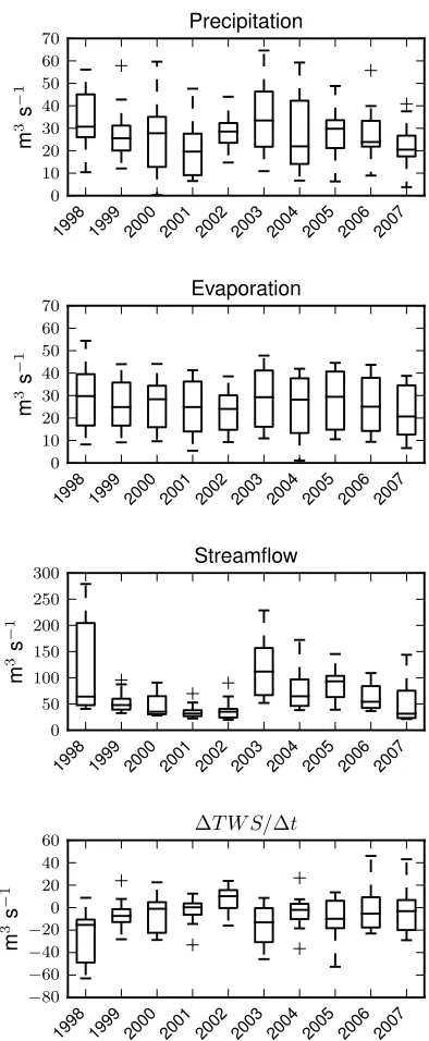
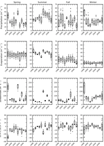
Box and whisker plots of average monthly conditions for all sub-watersheds show the distribution of precipitation, evapotranspiration, and streamflow values for the study period when viewed on both an annual scale (Figure 3.2) and on a seasonal scale (Figure 3.3). In the plots, the box represents the 25th_{, 50}th _{and 75}th_{percentiles of the}

distribution while the whiskers represent the minimum and maximum values. Outliers identified as data values more than 1.5 times larger or smaller of the Interquartile Range (IQR) are represented in the plots as “+” marks. Seasonal variability of streamflow in particular provides clear evidence of the 1998-2002 drought in spring, summer, and fall months. During these periods, the entire distribution of streamflow values was lower compared to the distribution of streamflow values during the years following the drought.

(44)

1998 1999 2000 2001 2002 2003 2004 2005 2006 2007 0 10 20 30 40 50 60 70 m 3s − 1 Precipitation

1998 1999 2000 2001 2002 2003 2004 2005 2006 2007 0 10 20 30 40 50 60 70 m 3s − 1 Evaporation

1998 1999 2000 2001 2002 2003 2004 2005 2006 2007 0 50 100 150 200 250 300 m 3s − 1 Streamflow

1998 1999 2000 2001 2002 2003 2004 2005 2006 2007

−80 −60 −40 −20 0 20 40 60 m 3s − 1

∆T W S/∆t

Figure 3.2: Annual variations (box with 25th_{, 50}th_{, and 75}th _{percentiles, whiskers}

(45)

1998 2000 2002 2004 2006 0 10 20 30 40 50 60 70 Pr ec ipi ta tio n (m

3 s

−

1)

Spring

1998 2000 2002 2004 2006 0 10 20 30 40 50 60 70 Summer

1998 2000 2002 2004 2006 0 10 20 30 40 50 60 70 Fall

1998 2000 2002 2004 2006 0 10 20 30 40 50 60 70 Winter

1998 2000 2002 2004 2006 0 10 20 30 40 50 60 70 Ev ap or at ion (m

3 s

−

1)

1998 2000 2002 2004 2006 0 10 20 30 40 50 60 70

1998 2000 2002 2004 2006 0 50 100 150 200 250 300 St re am flo w (m

3 s

−

1)

1998 2000 2002 2004 2006 0 50 100 150 200 250 300

1998 2000 2002 2004 2006 80 60 40 20 0 20 40 60 ∆ TW S/ ∆ t ( m 3s − 1)

1998 2000 2002 2004 2006 80 60 40 20 0 20 40 60

(46)

control volume is related to one or more time series that describe either an inflow or outflow for that control volume through time. Because control volumes and time series are georeferenced, it is possible to determine the mass flux into and out of each control volume through time. For example, the precipitation and evaporation fields were averaged over watersheds areas as

{P, E}= 1

T Z

{p, e}dA (3.8)

whereP is the precipitation into a watershed andE is the evapotranspiration exiting a watershed and both are expressed in flow rate dimensions [m3 _s−1_],_A_{is the area of}

a given watershed [m2_],_p_{is monthly precipitation and}_e_{is the monthly}

evapotranspi-ration for the sub-watershed accumulated over the time periodT [s] and expressed in length dimensions [m]. The organization of the data within the data model facilitated our ability to write code to estimate rate of change in TWS on a monthly time step using a discrete approximation of Equation 3.7 to estimate changes in TWS for all sub-watersheds identified in the study region.

3.5 Results and Discussion

3.5.1 Annual Variations of Rate of Change in TWS

(47)

Table 3.2: Annual rate of change in terrestrial water storage (m3 _s−1_{) for all}

sub-watersheds.

Year Avg STD Min 25% Med 75% Max

1998 -26.9 25.0 -63.0 -48.9 -15.3 -10.7 8.8

1999 -6.5 13.9 -28.2 -12.9 -7.4 -1.3 24.0

2000 -4.4 17.9 -28.8 -22.4 -1.0 4.9 22.5

2001 -2.7 11.9 -33.2 -6.3 0.3 3.8 12.4

2002 7.0 12.8 -16.0 -0.3 10.2 15.6 23.8

2003 -16.2 18.8 -45.8 -30.7 -13.1 -0.4 8.7

2004 -4.0 15.5 -36.5 -10.2 -2.0 3.4 26.4

2005 -10.3 18.7 -52.7 -18.2 -9.9 6.1 13.6

2006 -0.9 20.3 -23.0 -17.7 -5.4 9.3 46.1

2007 -3.2 21.6 -29.0 -20.0 -3.1 6.8 43.1

1

losing water during this period of time, but doing so less rapidly until the end of the drought (2001 and 2002) when the sub-watersheds actually began to gain water.

(48)

Table 3.3: Seasonal rate of change in terrestrial water storage (m3 _s−1_{) for all}

sub-watersheds.

Spring (March to May) Summer (June to August)

Year Avg STD Min 25% Med 75% Max Avg STD Min 25% Med 75% Max

1998 -56.3 9.1 -63.0 -61.5 -60.0 -52.9 -45.9 -22.0 15.8 -40.2 -26.7 -13.3 -12.9 -12.6

1999 -17.3 9.4 -28.2 -20.2 -12.2 -11.9 -11.5 -8.8 6.1 -14.7 -12.0 -9.3 -5.9 -2.5

2000 -21.9 8.8 -28.8 -26.9 -25.0 -18.5 -11.9 0.0 2.1 -2.2 -1.0 0.2 1.1 2.0

2001 -11.8 22.9 -33.2 -23.8 -14.5 -1.0 12.4 -2.0 5.9 -8.4 -4.6 -0.8 1.2 3.2

2002 -5.0 13.1 -16.0 -12.3 -8.5 0.5 9.5 6.2 16.3 -8.3 -2.6 3.1 13.5 23.8

2003 -25.0 22.8 -45.8 -37.1 -28.4 -14.5 -0.6 -31.9 13.7 -41.9 -39.7 -37.5 -26.9 -16.2

2004 -14.4 5.6 -18.4 -17.6 -16.8 -12.4 -8.0 9.4 14.9 -1.6 0.9 3.4 14.9 26.4

2005 -26.4 23.2 -52.7 -35.2 -17.8 -13.3 -8.7 -14.1 5.6 -19.5 -17.0 -14.4 -11.4 -8.3

2006 -19.6 3.0 -23.0 -20.7 -18.4 -17.9 -17.5 2.0 19.9 -19.2 -7.0 5.2 12.7 20.1

2007 -24.5 7.2 -29.0 -28.6 -28.2 -22.2 -16.2 4.2 6.8 -3.2 1.2 5.7 7.9 10.1

Fall (September to November) Winter (December to February)

Year Avg STD Min 25% Med 75% Max Avg STD Min 25% Med 75% Max

1998 -7.9 6.4 -15.3 -10.1 -4.8 -4.3 -3.7 -21.5 33.8 -57.9 -36.6 -15.3 -3.3 8.8

1999 4.6 16.8 -5.5 -5.0 -4.6 9.7 24.0 -4.7 16.9 -24.0 -10.9 2.2 5.0 7.7

2000 4.0 22.7 -21.8 -4.3 13.2 16.9 20.7 0.1 23.5 -24.3 -11.1 2.1 12.3 22.5

2001 0.3 5.5 -5.6 -2.2 1.3 3.3 5.3 2.5 3.8 0.2 0.3 0.4 3.6 6.8

2002 16.0 5.8 11.0 12.9 14.8 18.5 22.3 10.8 8.0 2.3 7.1 11.9 15.1 18.2

2003 -7.7 13.1 -19.5 -14.7 -9.9 -1.8 6.3 -0.3 9.2 -9.7 -4.7 0.2 4.4 8.7

2004 -11.8 21.6 -36.5 -19.4 -2.4 0.5 3.4 0.9 5.9 -3.7 -2.4 -1.1 3.2 7.5

2005 -1.1 23.1 -27.8 -8.4 10.9 12.3 13.6 0.4 10.1 -11.2 -2.6 5.9 6.3 6.6

2006 22.0 20.9 8.6 10.0 11.3 28.7 46.1 -8.1 4.9 -13.7 -10.0 -6.3 -5.4 -4.5

2007 6.4 15.0 -3.0 -2.3 -1.5 11.1 23.6 1.0 36.4 -20.2 -20.0 -19.9 11.6 43.1

1

3.5.2 Seasonal Variations of Rate of Change in TWS

Box and whisker plots of average monthly rate of change in TWS show the seasonal distribution of these values for the study period on an annual time scale (Table 3.3; Figure 3.3). While the winter and summer seasons showed more variability between different years of the study period, the fall season was in general a period of positive ∆T W S/∆tand spring was a period of negative ∆T W S/∆t. This result was expected because fall months tend to be a period of aquifer recharge in the state (measured by increases in groundwater levels, as shown later in this section), whereas spring months tend to be, in general, a period when groundwater levels decrease in large part to higher evapotranspiration rates.

(49)

in ∆T W S/∆t for each year of the drought. For the spring and summer months, although the rate of change in ∆T W S/∆t increased, it remained negative or close to zero. We suspect that this is a result of a loss of TWS during the drought so that in later years of the drought, TWS was low so ∆T W S/∆t approached zero. In the fall months, there is no clear pattern in ∆T W S/∆t between drought and non-drought years. This is likely due to the fact that fall months experienced near normal precipitation rates. In the winter months during the drought years, there was a large variation in the rate of change in TWS compared to the non-drought years. The winter period of the drought years also had a large variation in precipitation, which would explain the large variation in TWS change rates. However, the 75th _percentile

for precipitation in the winter months was inline with that of months following the period of drought, and the 75th _{percentile for ∆}_{T W S/}_∆_t_{during the winter months of}

the drought years was lower compared to non-drought years. A possible explanation for this result is a higher antecedent soil moisture condition in the winter months, due to the proceeding fall season that was found to be the primary period of increases in TWS.

3.5.3 Spatial Variations in Annual and Seasonal Rate of Change in

TWS

(50)

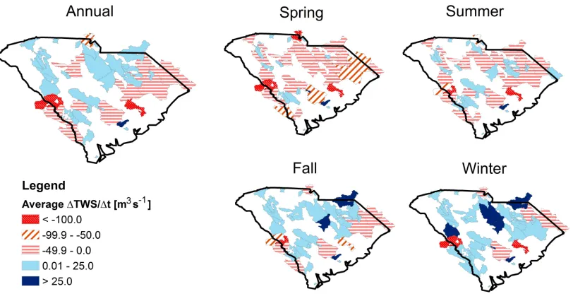
Figure 3.4: Spatial variation of rate of change in terrestrial water storage in the sub-watersheds.

will contribute more to recharge aquifers in the inland portion of the state relative to stream discharge. In contrast, groundwater will be a larger contributor to streamflow in the coastal region of the state, meaning stream discharge will be larger thanP−E

and, as a result, ∆T W S/∆t will tend to be positive. For sub-watersheds in Blue Ridge and Piedmont region, as well as the Southeastern Coastal Plain regions, as expected, the fall months showed a positive rate of change in terrestrial water storage for most of the sub-watersheds, while spring months showed a deficit for most of the sub-watersheds.

Within these general trends there was some variability. For example, one sub-watershed near the coast gained water consistently throughout the year at a rate that exceeded 25 m3 _s−1_{. Four sub-watersheds distributed throughout the study region}

lost water during all four seasons, two at a rate that exceeded 100 m3 _s−1_{. There}

(51)

For example sub-watersheds with reservoirs may have ∆T W S/∆t <0 because they released water during drought years that was stored prior to the drought. If a reservoir stores water, the ∆T W S/∆t increases because Qin > Qout and therefore R < 0.

When the reservoir later releases water, the ∆T W S/∆tdecreases becauseQout > Qin,

and thereforeR >0. For sub-watersheds where reservoirs must be accounted for rate of change in TWS, information is needed about reservoir volume through time and how the reservoir released water through time. Three of the sub-watersheds with negative annual rate of change in TWS for the study period are near cities in the study region: Charlotte, North Carolina; Charleston, South Carolina; and Augusta, Georgia. Another possible explanation, therefore, is that there is significant surface water diversion for public or industrial water use in these regions of the state. Both of these examples suggest that human influences could be responsible for abnormal rate of change in TWS rates for the study region. Future work that includes other datasets related to water use for human and industrial purposes is needed to test this hypothesis.

3.5.4 Comparison of Cumulative Rate of Change in TWS Estimates

with Observed Groundwater Levels

(52)

G H

C E

D

A

F

B

NC

GA

0 30 60 120Kilometers

´

Legend

Groundwater Observation Focus Subwatersheds

.

Figure 3.5: Location of the focus sub-watersheds in South Carolina.

storage (reservoirs), surface water diversions for public water supply or industrial wa-ter use, or simply a disconnect between surface wawa-ter and groundwawa-ter resources could impact the two variables and remove any correlation between them. Therefore, we expected some sub-watersheds to show clear correlation between ∆T W S/∆t and GWL, while at the same time we expected other sub-watersheds to show no correla-tion. In some ways, this analysis is most helpful in identifying sub-watersheds where GWL and cumulative ∆T W S/∆tdo not match because it suggests some other factor, possibly anthropogenic, may be altering the local water budget for that particular sub-watershed.

(53)

Jan Feb Mar Apr MayJun Jul Aug Sep Oct NovDec 0 10 20 30 40 50 60

70 ₉_.₀

9.1 9.2 9.3 9.4 9.5 9.6 9.7 9.8

Watershed H(R2_{= 0.11)} Jan Feb Mar Apr MayJun Jul Aug Sep Oct NovDec

−140 −120 −−10080 −60 −40

−200 1.00

1.05 1.10 1.15 1.20 1.25

Watershed A(R2_{= 0.87)}

Jan Feb Mar Apr MayJun Jul Aug Sep Oct NovDec −250 −200 −150 −100 −50 0 50

11.4 11.6 11.8 12.0 12.2 GWL

(m)

Watershed D(R2_{= 0.62)}

Jan Feb Mar Apr MayJun Jul Aug Sep Oct NovDec −60 −40 −20 0 20 40

60 ₄₈_.₆₆

48.68 48.70 48.72 48.74 48.76 48.78 48.80

Watershed F(R2_{= 0.68)}

Jan Feb Mar Apr MayJun Jul Aug Sep Oct NovDec 10 20 30 40 50 60 70

0.90

0.95

1.00

1.05

Watershed G(R2_{= 0.24)} Jan Feb Mar Apr MayJun Jul Aug Sep Oct NovDec −600 −500 −400 −300 −200 −100 0 Cumulativ e ∆ T W S/ ∆ t ( m 3s − 1)

14.6 14.8 15.0 15.2 15.4 15.6 15.8 16.0 16.2

Watershed C(R2_{= 0.46)}

Jan Feb Mar Apr MayJun Jul Aug Sep Oct NovDec −20

−100 10 20 30 40 50

60 10.8

10.9 11.0 11.1 11.2 11.3 11.4 11.5 11.6

Watershed B(R2_{= 0.20)}

Jan Feb Mar Apr MayJun Jul Aug Sep Oct NovDec −50

−40 −30 −20 −100 10 20

30 ₁₀_.₅

10.6 10.7 10.8 10.9

Watershed E(R2_{= 0.08)}

Cumulative∆TWS/∆t (m3_s−1₎ _{GWL (m) from Surface}

(54)

GWL. On the other hand, sub-watersheds B, E, G and H did not show a clear correlation. In some cases, this lack of correlation appeared to be due to a phase shift between cumulative ∆T W S/∆t and GWL. This phase shift may be related to the travel time through the soil to the aquifer including parameters such as the depth from the land surface to the saturated soil and the characteristics of the soil column (hydraulic conductivity, antecedent soil moisture, etc.). Sub-watershed B’s groundwater level pattern appeared to be influenced by pumping, and there is some documentation on pumping in this sub-watershed (USDI and USGS, 2009). It is possible that this pumping affected the correlation between GWL and cumulative ∆T W S/∆t. In other cases, in particular for sub-watersheds E, G, and H, ∆T W S/∆t

showed an increase during fall months that was not present in the GWL observations. Again, further work is needed to understand the specific characteristics and factors present in these sub-watersheds in order to explain divergence between ∆T W S/∆t

and GWL. The seasonal variations were also visible in this analysis with the tendency of the groundwater level to rise in the fall and winter months and to decrease in spring and summer months, as expected.

When viewed as a time series with rate of changes in TWS accumulated during the year (Figure 3.7), it is possible to visualize the increase or decrease in ∆T W S/∆t

(55)

Jan-98 Jan-99 Jan-00 Jan-01 Jan-02 Jan-03 Jan-04 Jan-05 Jan-06 Jan-07 40 200 20 40 60 80 100 120 _8.5 9.0 9.5 10.0 10.5 Watershed H

Jan-98 Jan-99 Jan-00 Jan-01 Jan-02 Jan-03 Jan-04 Jan-05 Jan-06 Jan-07 400

300 200 1000 100

200 0.9_1.0

1.1 1.2 1.3 1.4 1.5 1.6 Watershed A

Jan-98 Jan-99 Jan-00 Jan-01 Jan-02 Jan-03 Jan-04 Jan-05 Jan-06 Jan-07 800 600 400 2000 200 10.5 11.0 11.5 12.0 12.5 13.0 13.5 Watershed D

Jan-98 Jan-99 Jan-00 Jan-01 Jan-02 Jan-03 Jan-04 Jan-05 Jan-06 Jan-07 300 200 1000 100 200 300 400 500 47.5 48.0 48.5 49.0 49.5 Watershed F

Jan-980 Jan-99 Jan-00 Jan-01 Jan-02 Jan-03 Jan-04 Jan-05 Jan-06 Jan-07 20

40 60

80 0.60.7_0.8

0.9 1.0 1.1 1.2 1.3 1.4 Watershed G

Jan-98 Jan-99 Jan-00 Jan-01 Jan-02 Jan-03 Jan-04 Jan-05 Jan-06 Jan-07 1400 1200 1000800 600 400 2000 200 Ye ar ly Cu m ula tiv e ∆ TW S/ ∆ t ( m 3s − 1) 10 12 14 16 18 GWL (m) Watershed C

Jan-98 Jan-99 Jan-00 Jan-01 Jan-02 Jan-03 Jan-04 Jan-05 Jan-06 Jan-07 40 200 20 40 60 80 100

120 10.8_11.0

11.2 11.4 11.6 11.8 12.0 12.2 12.4 Watershed B

Jan-98 Jan-99 Jan-00 Jan-01 Jan-02 Jan-03 Jan-04 Jan-05 Jan-06 Jan-07 10080 60 40 200 20 40 60 10.0 10.5 11.0 11.5 12.0 Watershed E

Yearly Cumulative ∆TWS/∆t (m3s−1) GWL (m)

(56)

the study period, but also showed evidence of the drought in 1998 and 2003 because there was little or no increase in ∆T W S/∆t during these years, whereas other years in the study period showed an increase in ∆T W S/∆t throughout the year. One pattern of interest is the increase in ∆T W S/∆t that occurred directly following the drought in 2002. This increase in ∆T W S/∆t is evident from the time series plots for sub-watersheds B, E, G, and H and match increases in the groundwater level that also occurred during this time period. What is also clear from this plot is the marked difference in how each sub-watershed responded during and following the period of drought. Some sub-watersheds gained ∆T W S/∆t during drought years, others lost water. Some sub-watersheds gained ∆T W S/∆tin years following the drought, others lost water. This provides evidence of the variability of hydrologic systems that are under influences from geologic, climate, human, and other dimensions.

3.6 Conclusion

(57)

of the state responded during and following the period of drought, information that may prove useful in managing the state’s water resources.

We found that the method was most valuable in its ability to identify sub-watersheds in the state that do not follow general spatial and temporal variations. There could be many factors at play that result in these abnormalities. In some cases, there could be an internal storage (e.g., reservoir) that is altering storage rates relative to neighboring sub-watersheds. In other cases, there could be an unaccounted source or sink for water within the sub-watershed. For example, there may be an inter-watershed transfer of water or a diversion of surface water for public industrial water use purposes. These abnormalities, therefore, suggest that there is a human dimension to the water balance for that particular sub-watershed. Future work should further investigate this finding by gathering other water use data in an attempt to close the water balance for these sub-watersheds.

(58)

(59)

Chapter 4 Comparison of VIC and MODIS-derived

evapotranspiration estimates for closing

regional-scale water balances

1

4.1 Abstract

Two approaches for quantifying evapotranspiration (ET) were evaluated in terms of their ability to close regional scale water balances: (i) simulation using the Variable Infiltration Capacity (VIC) model and (ii) a Moderate Resolution Imaging Spectro-radiometer (MODIS) derived approach described by Mu et al. (2011). ET products from the two approaches served as input to a water balance framework that incorpo-rates observed streamflow and precipitation estimates for 44 sub-watersheds in South Carolina to estimate changes in water storage on a monthly time step over time period from 2000 to 2007. Two methods were used to evaluate the results of water balance calculations. In the first method, storage change estimates based on two ET prod-ucts were compared with the Gravity Recovery and Climate Experiment (GRACE) Terrestrial Water Storage (TWS) change product. Based on this first method for evaluation, ET estimates from VIC were found to produce water storage estimates that most closely matched those obtained by GRACE. In the second method for eval-uation, storage change estimates for the two ET approaches were evaluated based on

(60)

their correlation with monthly groundwater level observations. This second method for evaluation showed evidence that ET estimates derived from MODIS are better correlated with fluctuations in groundwater levels. However, this second method for evaluation may favor MODIS because it produced lower ET estimates that resulted in an emphasis on streamflow and precipitation in the water balance framework, and not because it produced more accurate ET estimates. Therefore, the first method for evaluation was weighted more strongly and the conclusion from this study is that VIC derived ET estimates were closer to actual ET estimates for the evaluated study region and period of analysis.

4.2 Introduction

(61)

per-form such an analysis by using an observation-based water balance framework for a set of watersheds in South Carolina.

This work is an extension of our prior work (Billah and Goodall, 2011) where we used the North American Regional Reanalysis (NARR) product for estimating ET within a similar regional-scale water balance framework. We found through this work that NARR tended to overestimate ET rates, resulting in an unrealistic decrease in storage over the decade period of analysis. This result, which has been shown by others as well [e.g., Ruiz-Barradas and Nigam, 2006a; Zeng et al., 2008], is typically handled by applying a correction factor to NARR ET estimates to ensure no net change in long term storage. The need for this correction is not ideal. Furthermore, NARR estimates are at a coarse spatial scale for watershed studies (32.6 km), mak-ing the product unable to capture small-scale variability in ET rates important for regional hydrologic analysis. While downscaling approaches (e.g., Wood et al., 2004) could be used to improve the spatial resolution of NARR output for use in hydrologic analysis, NARR ET would still require the use of a bias-correction factor to ensure no net change in long term water storage. Therefore we concluded through our previous work that improved estimates of ET using alternative approaches are necessary to better quantify the rate of change in water storage.

(62)

& & & & ! !

#

*

#

*

78°W 78°W 79°W 79°W 80°W 80°W 81°W 81°W 82°W 82°W 83°W 83°W 36°N 36°N 35°N 35°N 34°N 34°N 33°N 33°N 32°N 32°N

0 25 50 100km

AND-326 OC-233 HAM-083 MLB-112

.

Legend

#

*

SCAN Station ! USGS Stream Gage

Site A Site B

& _{Groundwater Wells}

Pee Dee Basin Catawba Basin Broad/Saluda Basin Savannah Basin USGS 02156500 USGS 02135000 SCAN 2037 SCAN 2038

Figure 4.1: The study area including the sub-watersheds for which change in stor-age has been estimated grouped into four major river basins (Pee Dee, Catawba, Broad/Saluda, and Savannah). Also shown are the locations of groundwater wells, soil moisture networks, stream gaging stations used for model evaluation.

(63)

datasets: Gravity Recovery and Climate Experiment (GRACE) TWS estimates and groundwater levels. Our methodology, therefore, provides a means for quantifying the accuracy of the ET estimates by how well they are able to estimate changes in water storage for the study region measured independently by GRACE and groundwater level observations. Details of modeling approach and methods used to perform the analysis follow.

4.3 Methods and Materials

4.3.1 Water Balance Framework

The rate of change in water storage for a given sub-watershed can be calculated as

(

∂T W S ∂t

)

={Pobs} − {ETest}+{Rin} − {Rout} (4.1)

where∂T W S/∂tis the rate of change in water storage within that sub-watershed,Pobs

is observed precipitation, Eest is an estimated evapotranspiration, Rin is streamflow

entering to the sub-watershed and Rout is streamflow exiting the sub-watershed. The

brackets around these terms signify a spatial average over the sub-watershed area and the bar signifies a temporal average over a month time period. Equation 4.1 was applied for all sub-watersheds in the study area for which the stream inflow (if not a headwater stream) and outflow were observed over the period of study (2000-2007). We adopted this approach from Zhang et al. (2008), who applied a similar approach in the Amazon and the Mississippi River Basins.

(64)

Jan-00 Jan-01 Jan-02 Jan-03 Jan-04 Jan-05 Jan-06 Jan-07

0.0 0.1 0.2 0.3 0.4 0.5

0.1 0.2 0.3 0.4 0.5

(a) Overall Study Area

0.0 0.1 0.2 0.3 0.4 0.5

Monthly A verage Streamflo w (m)

0.1 0.2 0.3 0.4 0.5

Monthly

A

verage

Precipitation

(m)

(c) Catawba Basin

0.0 0.1 0.2 0.3 0.4 0.5

0.1 0.2 0.3 0.4 0.5 0.6

(e) Savannah Basin

0.0 0.1 0.2 0.3 0.4 0.5

0.1 0.2 0.3 0.4 0.5

(b) Pee Dee Basin

0.0 0.1 0.2 0.3 0.4 0.5

0.1 0.2 0.3 0.4 0.5 0.6

(d) Broad/Saluda Basin

Figure 4.2: Monthly precipitation and streamflow averaged for (a) all sub-watersheds in the study area and (b-e) for the four major river basins in the study area. Stream-flow and precipitation have been normalized by sub-watershed area and therefore are expressed in length units.

(65)

sub-watersheds define incremental drainage area between streamflow gaging stations. The methodology for delineating the sub-watersheds in this paper improves on our previous approach which relied on NHD Plus catchments instead of flow direction and accumulation grids.

We obtained estimates of precipitation and streamflow for each of the sub-watersheds using spatial analysis routines available in GIS software as described in detail in Billah and Goodall (2011) and summarized here (Figure 4.2). Precipitation for each sub-watershed was estimated from the Parameter-elevation Regressions on Independent Slopes Model (PRISM) dataset (Gibson et al., 2002). PRISM provides grided precipitation estimates on a 4 km spatial resolution and on a monthly time step. Monthly average streamflow was obtained from the United States Geologic Survey (USGS) for the gauges with complete records over the period of analysis. Monthly ET was estimated using the approaches described in the following sub-sections. Finally, we used the geospatial-temporal data model described by Goodall and Maidment (2009) to organize the data for later processing.

4.3.2 Estimating ET using VIC

VIC is a semi-distributed macro-scale model that performs water and energy balances for a grid-based discretization of the landscape (Liang et al., 1994, 1996). The water balance equation used in VIC can be stated as

∂S

∂t =P −ET −R (4.2)

Quantifying Regional-Scale Water Storage Using Models and Observations: Application For Drought Assessment In South Carolina

University of South Carolina

Scholar Commons

Quantifying Regional-Scale Water Storage Using

Models and Observations: Application For

Drought Assessment In South Carolina

Mirza Md Mozaddid Billah

Dedication

Acknowledgments

Abstract

Table of Contents

List of Tables

List of Figures

Chapter 1

Introduction

Chapter 2

Background

2.1

The Impact of the 1998-2002 Drought on South

Car-olina Water Resources

2.2

Water Balance Framework

2.3

Evapotranspiration

2.4

Data Management Cyberinfrastructure

Chapter 3

Annual and interannual variations in

terrestrial water storage during and

following a period of drought in South

Carolina, USA

3.1

Abstract

3.2

Introduction

3.3

Study Area

3.4

Methodology

3.5

Results and Discussion

1

´

.

3.6

Conclusion

Chapter 4

Comparison of VIC and MODIS-derived

evapotranspiration estimates for closing

regional-scale water balances

4.1

Abstract

4.2

Introduction

#

*

#

*

.

#

*

4.3

Methods and Materials