Title: Lossless Compression of Images Using Row-Column Reduction Coding

(1)

265

Available Online atwww.ijcsmc.com

International Journal of Computer Science and Mobile Computing

A Monthly Journal of Computer Science and Information Technology

ISSN 2320–088X

IMPACT FACTOR: 5.258

IJCSMC, Vol. 5, Issue. 3, March 2016, pg.265 – 272

Lossless Compression of Images Using

Row-Column Reduction Coding

Aarthi.D

1

, Balaji.R

2

¹Student, Department of Computer Science and Engineering, Sri Krishna College of Engineering and Technology, India 2

Assistant Professor, Department of Computer Science and Engineering, Sri Krishna College of Engineering and Technology, India 1

aarthideva06@gmail.com; 2 balajir@skcet.ac.in

Abstract— Image compression deals with the reduction of irrelevance and redundancy of the image such that it helps in efficient transmission of data. The objective of the proposed method is to present an advanced method for lossless compression of images. The images include map images, graphics, as well as binary images. The proposed method presents an efficient image compression approach based on two main components. The first component is a codebook encompassing 8 × 8 bit blocks of data. The fixed part consists of 8 × 8 blocks and the variable part comprises of codes corresponding to the blocks. The image is converted to a monochrome image before the generation of codebook. The size of the codebook is very less. Hence, some blocks from input images cannot be compressed via the codebook. Hence, the second component, the Row-Column Reduction Coding (RCRC) was being designed. RCRC is an iterative algorithm and helps to compress 8 × 8 blocks of a binary matrix, which are not in the codebook. This method removes redundancy between row vectors of a block using the Row-Reference Vector (RRV) and column vectors of a block using the Column-Reference Vector (CRV). This means that the quality of the image is almost retained without high loss of data. Hence, the image obtained after applying the proposed compression technique will be a lossless image. The original image and the image obtained after compression are to be compared to calculate the ratio of compression and also the quality of the image after compression.

Keywords— lossless, compression, binary images, colour images, blocks.

I. INTRODUCTION

(2)

266

Fig. 1 Basic image compression architecture

Image compression may be lossy or lossless. Lossless compression is preferred for archival purposes and often for medical imaging, technical drawings, clip art, or comics. Lossy compression methods, especially when used at low bit rates, introduce compression artifacts. Lossy methods are especially suitable for natural images such as photographs in applications where minor (sometimes imperceptible) loss of fidelity is acceptable to achieve a substantial reduction in bit rate. The lossy compression that produces imperceptible differences may be called visually lossless.

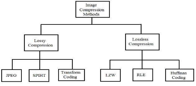
The work demonstrates a new innovative method for lossless compression of images such as binary images as well as discrete-color images. The method consists of 8 x 8 blocks that are non-overlapping. The binary images collected are partitioned into 8 x 8 blocks for analyzing of the overall entropy of the system. The entropy coders are the Huffman coding and Arithmetic coding algorithms. Either of the one code is used as a pair with 8 x 8 blocks of the image in order to form a codebook. The images that contain salt-and-pepper noise are eliminated. The relative probabilities of all blocks are used to calculate the entropy of the images. Huffman codes and Arithmetic codes are constructed for all blocks of the binary image with the help of the probability distribution of 8 x 8 blocks. Fig. 2 shows the classification of image compression methods.

Fig, 2 Classification of Image Compression methods

Section II briefly describes the proposed compression method in detail. Section III explains about the areas of application of the method. This section also provides the compression results based on two encoding schemes. Section IV deals with the Conclusion and Future Work.

II. PROPOSED METHOD

The main idea of the proposed method is to partition the binary image into non-overlapping blocks of size 8 x 8. The process of partitioning the binary images into blocks and encoding the blocks is basically referred to as block coding. Here, the images are partitioned into blocks of black and white pixels. The black corresponds to the value 0 and white corresponds to the value 1.

A. The Codebook Model

The codebook model encompasses 8 × 8 bit blocks of data along with their corresponding probabilities of occurrence. This method operates on a fixed-to-variable codebook. The fixed part consists of 8 × 8 blocks and the variable part comprises codes corresponding to the blocks as summarized in [1]. This can be utilized for compressing efficiently all types of binary images. The images have different sizes, such as fingerprints and natural sceneries. The candidates were extracted from different sources, such as randomly browsed web pages.

(3)

267

Another step in pre-processing is to make the image width and height divisible by 8. Let w and h represent the width and height of the image respectively. w and h are converted into w* and h* such that 8|w* and 8|h* are as follows in (1) and (2):

If , then (1)

If , then (2)

Hence, w* x h* forms the new dimensions. The problem of determining the waiting probability of observing a particular number of blocks and the expected number of samples needed may be viewed at an instance of the Coupon-Collector‟s Problem that is explained in [4] as follows:

Let S denote the set of coupons (or) items, having cardinality |S| = N. Coupons are collected with replacement from S. Let M denote the set of observed coupons and T be a random variable. More accurately, M is a multiset of coupons because the coupons are drawn from S with replacement. The probability of collecting more than n coupons, i.e. P(T > n) is given in (3). This is summarized in [1]. Hence, the required probability P(T = n) is easily derived as P(T = n) = P(T > n − 1)−P(T > n). The following model gives P(T > n):

(3)

To determine the expected number of trials, E [T], required to collect n coupons, the model E [T] = nHn, where Hn is the harmonic number is used. Based on the asymptotic expansion of harmonic numbers, the following asymptotic approximation for E [T] as specified in (4) holds:

(4)

where γ ≈ 0.577 is the Euler-Mascheroni constant. If n=264 coupons, then the expected number of trials bounded by equation (4) is equal to 8.29×1020, which implies a practically unattainable number of trials.

The observed average code length, L, is given by the equation (5) as follows,

(5)

where, qi is the empirical distribution and N is the number blocks. Similarly, the theoretical average code length for the

theoretical probabilities pi is as follows in (6):

(6)

The model is examined as represented in (7).

(7)

The codebook that is constructed acts as the static modelling portion of the compression method. The representative codes are constructed for most of the symbols that are collected from modelling. The complexity of the decoder is reduced by the static modelling. But, it is not widely used in practice because sample data may not always be representative of all data. The analysis on the constructed codebook suggests a small lower bound and a small asymptotic upper bound on the discrepancy between theoretical and empirical code lengths. Moreover, a compression model has been based on a fixed-to variable codebook. Huffman and Arithmetic coding are used to implement the coder section.

B. The Row-Column Reduction Coding (RCRC)

The Row-Column Reduction Coding is an iterative algorithm. This coding method helps to remove the redundancy between row vectors and column vectors of a block. For each 8 × 8 block RCRC generates r, which represents the row reference vector (RRV), and c, which represents column reference vector (CRV as cited in [1]. Vectors r and c may be viewed as 8-tuples which can acquire values 0 ≤ ri ≥ 1, 0 ≤ ci ≥ 1 and 1 ≤ i ≥ 8. A comparison between pairs of rows and columns from the block b is done

(4)

268

then the first pair of vector is kept for future use and the second pair of vector is eliminated, the second pair of vector corresponds to the duplicate pair. The final vector contains the reduced block. If the vectors in the given pair are not identical, then both of the vectors are preserved. The preserved vector pairs of rows and columns are stored in RRV and CRV, respectively.

Let bi, j denote row i of block b, for 1 ≤ j ≥ 8. The starting first two rows of the block (b1, j, b2, j) are compared first with the

help of RCRC. If b1, j= b2, j, then it indicates that the two rows of the block are identical. Hence the first row r1 is assigned a

value 1 and the second row r2 is assigned a value 0. Hence the row b2, j is eliminated from the block b. Now, the first block b1, j is

compared to the next block b3, j. If both the blocks are equal, the row r3 is assigned a value of 0, implying that the corresponding

row is being rejected from the block. As both the rows are not identical, the row r3 is assigned a value of 1. Hence, RCRC takes

a new pair of rows (b3, j, b4, j) and the comparison is proceeded for those two rows. The procedure is iterated until RCRC

compares all the rows of the block till the final row of the block, taking into account the successive sets of rows, as summarized in [1].

By the rule, when an i-th row in the block is assigned 1, it means that the row ri is upheld and when an i-th row in the block

is assigned 0, it means that the row ri is rejected. The output of these procedures will be row-reduced block. Next, the column

reference vector is constructed based on the row-reduced block using RCRC. The output produced with the help of column reference vector is the column-reduced block. The final outcome of the operations is the row-column-reduced block.

Fig. 3 The row-reduction operation applied on a selected block.

Fig. 3 explains the row reduction operation is applied on a selected block. In the row reference vector (RRV), the first two rows of the block are identical. Hence the second row is eliminated from the block. Therefore, the first row is assigned a value 1 and the second row is assigned a value 0. The row with the value 1 is preserved and the row with the value 0 is eliminated. Now, the first row is compared with the third row of the block. As both the rows are identical, the third row is also assigned a value of 1. On comparing the third row with the rest of the rows (from 4 to 8), all the rows from 4 to 8 are eliminated, as these rows contain redundant values.

Fig. 4 The column-reduction operation applied on the row-reduced block.

(5)

269

As the output contains two ones in each RRV and CRV, there will be two rows and two columns in the final reduced block. The first reduced row is represented by the first two bits of the reduced block „10‟. The second reduced row is represented by the second two bits of the reduced block „11‟. Finally, the ones and zeros present in the reference vectors are used in the reconstruction process of the original block with the help of rows and columns of the reduced block.

Fig. 5 The column reconstruction based on the column-reference vector.

In Fig. 5, the CRV conveys the message to the decoder that the column 1 has identical values to columns 2 to 6, and column 7 has an identical copy in column 8.

Fig. 6 shows the row reconstruction process to obtain the original block. If the output of the row–column reduction routine has a size larger than 64 bits, the original block is kept. Such cases represent less than 5% of the total block count in the test samples.

Fig. 6 Row reconstruction based on the row-reference vector (RRV).

Moreover, the minimum number of bits that can be achieved by RCRC is 17 bits, for a maximum compression ratio of 73.44%, and occurs in cases where all 7 rows and 7 columns of the block are eliminated which leads to 1 bit reduced block as cited in [1].

(6)

270

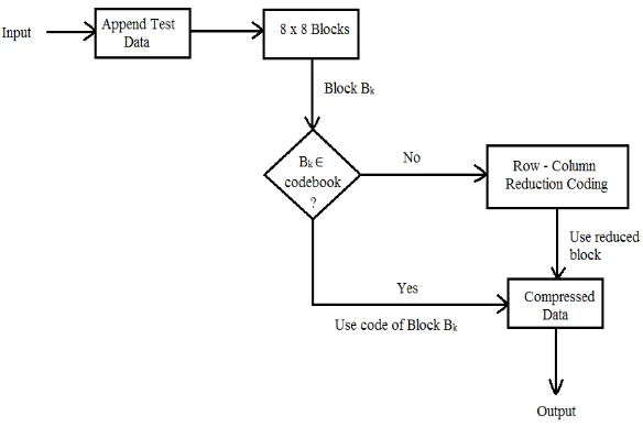
The schematic diagram shown in Fig. 7 illustrates the operation of the proposed compression scheme. Each image is modified in both dimensions to become divisible by 8. Then, layers are extracted through colour separation yielding a set of bi-level matrices. Each layer is partitioned into 8 × 8 blocks. Each 8 × 8 block of the original data is searched in the codebook. If it is found, the corresponding Run-Length code is selected and added to the compressed data stream. If it is not found, the row– column reduction coding attempts to compress the block.

III.APPLICATIONS

The proposed lossless compression method was tested on binary and discrete colour images. The empirical results of the compression have been reported. The comparison of the proposed algorithm is done with the existing Huffman Coding algorithm and the results are observed.

A. Binary Images

The proposed compression method was tested on variety of images which include both binary and discrete color images. These images were obtained from different sources, which include internet images also. These images are shown in the Fig. 8. In both the cases, a chosen set of images is given as an input along with the compression ratio of the proposed compression method using Run-Length Encoding and Huffman Coding.

Fig. 8 Binary images reported in empirical results

TABLE I

EMPIRICAL RESULTS FOR SELECTED BINARY IMAGES

Image Dimensions Ep Ep* AC JBIG2

001 192x188 88.57 90.25 90.88 86.24 002 201x194 86.24 89.98 90.21 84.21 003 302x214 89.54 94.67 94.55 88.65 004 351x257 88.35 92.36 93.11 86.98 005 203x164 96.85 98.22 98.28 93.24 006 684x541 92.24 94.44 94.24 91.88

Average 90.29 93.32 93.54 88.53

Table I displays six solid binary images along with their corresponding compression ratios. On considering Run-Length coding, the alternative encoding scheme produces better performance than the other encoding scheme. On an average, the proposed algorithm performs well on comparison with the standard Huffman coding algorithm by approximately 1.58%.

TABLE II

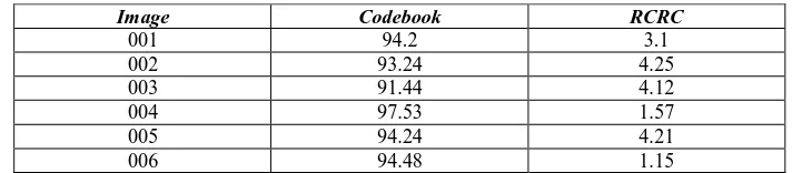
PERCENTAGE OF BLOCKS COMPRESSED BY THE CODEBOOK AND RCRC

Image Codebook RCRC

001 94.2 3.1

002 93.24 4.25

003 91.44 4.12

004 97.53 1.57

005 94.24 4.21

(7)

271

Table II shows the percentage of blocks compressed by the codebook dictionary and the percentage of blocks compressed by RCRC for the corresponding images.

B. Discrete-Colour Images

In accession to the binary images, the proposed method may be tested on discrete colour images also. These type of images consists of four semantic layers, such as, roads, rivers, lines and lakes.

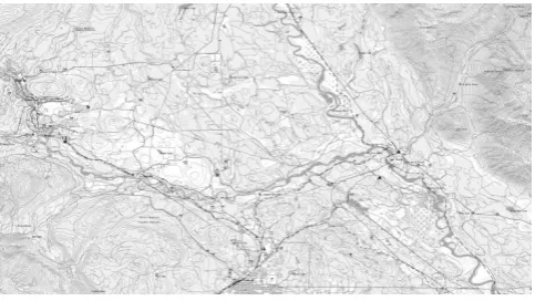
Fig. 9 Example of Colour Separation

Fig. 9 shows the separation of layers of a map image which is obtained from [5]. In this case, the map image contains four layers as stated in the above paragraph. Each colour is paired with the background colour to form a layer of bi-level images, as summarized in [6]. A program was developed to perform colour separation that contains same colour pixels. These are then treated as binary images and their corresponding compression ratios are coupled together in order to produce the final result for the images.

TABLE III

DESCRIPTION OF SELECTED MAP IMAGE

Map Dimensions Size(KB)

1 2654 1523

Table III provides a summary of map images used in the process. Table IV shows the compression results in bits per pixel (bpp) of the proposed method for the map images shown in Table III. From the results displayed in the tables, it may be concluded that the proposed method accomplishes high compression ratio on the selected map images.

TABLE IV

COMPRESSION RESULTS FOR MAP IMAGES USING THE PROPOSED METHOD

Map Compressed Size (KB) Compression Ratio (bpp)

1 190.77 0.29

The results of proposed method has been reported to compress at a rate of 0.31 to 0.22 bits per pixel (bpp). On average, the proposed method attains a compression of 0.425 bpp on maps. This result is higher than or comparable to those results reported in [4].

C. Run-Length Encoding

(8)

272

than relative frequencies for particular 8 x 8 blocks. The proposed method works efficiently with Run-Length Encoding, but somewhat incompatible probabilities are produced for the coder function as summarized in [3].

IV.CONCLUSION AND FUTURE WORK

This method has been successfully implemented on two major image categories: (i) images that consist of a predetermined number of color images, such as maps, graphs; and (ii) binary images. The image taken for generation of the codebook is first converted to a binary image. This binary image is further processed to store each pixel value of the image in the codebook. Each 8×8 block of the original data is searched in the codebook. If it is found, the corresponding Run-Length code is found and the corresponding code is added to the compressed data stream. If it is not found, the block is compressed with the help of row– column reduction coding. It involves the implementation of row-column reduction coding, which compresses the images resulting in lossless image after compression. Finally the compressed data is given as the resultant image. The results (i.e.,) the original image and the compressed images are to be compared to evaluate the ratio of the compression and also the quality of compressed image. This comparison is done with the help of PSNR. Future work of the project involves compression of images in motion (i.e.,) video compression.

REFERENCES

[1] Saif Alzahir, Member, IEEE, and Arber Borici, Student Member, IEEE, “An Innovative Lossless Compression Method for Discrete-Color Images”, IEEE Transactions on Image Processing, Vol. 24, NO. 1, January 2015.

[2] Mamta Sharma, “Compression Using Huffman Coding”, IJCSNS International Journal of Computer Science and Network Security, VOL.10 No.5, May 2010.

[3] Pratishtha Gupta, G.N Purohit, Varsha Bansal, “A Survey on Image Compression Techniques”, International Journal of Advanced Research in Computer and Communication Engineering Vol. 3, Issue 8, August 2014.

[4] W. Feller, “An Introduction to Probability Theory and Its Applications”, vol. 1, 3rd edition. New York, NY, USA: Wiley, 1968, p. 509.

[5] “Topographical Map of British Columbia”, Univ. Northern British Columbia, George, BC, Canada, 2009.