Forecasting peak load electricity demand using statistics and rule based approach

ISSN 1546-9239

© 2009 Science Publications

Corresponding Author: Zuhaimy Ismail, Department of Mathematics, Faculty of Science, University Technology Malaysia, 81310 UTM Skudai, Johor, Malaysia Tel: +60197133940 Fax: +6075566162

1618

Forecasting Peak Load Electricity Demand Using

Statistics and Rule Based Approach

1

Z. Ismail,

A.Yahya and

K.A. Mahpol

1

Department of Mathematics, Faculty of Science,

University Technology Malaysia, 81310 Skudai, Johor, Malaysia

2

Department of Foundation Education, Faculty of Education,

University Technology Malaysia, 81310 Skudai, Johor, Malaysia

Abstract: Problem statement: Forecasting of electricity load demand is an essential activity and an important function in power system planning and development. It is a prerequisite to power system expansion planning as the world of electricity is dominated by substantial lead times between decision making and its implementation. The importance of demand forecasting needs to be emphasized at all level as the consequences of under or over forecasting the demand are serious and will affect all stakeholders in the electricity supply industry. Approach: If under estimated, the result is serious since plant installation cannot easily be advanced, this will affect the economy, business, loss of time and image. If over estimated, the financial penalty for excess capacity (i.e., over-estimated and wasting of resources). Therefore this study aimed to develop new forecasting model for forecasting electricity load demand which will minimize the error of forecasting. In this study, we explored the development of rule-based method for forecasting electricity peak load demand. The rule-based system synergized human reasoning style of fuzzy systems through the use of set of rules consisting of IF-THEN approximators with the learning and connectionist structure. Prior to the implementation of rule-based models, SARIMAT model and Regression time series were used. Results: Modification of the basic

regression model and modeled it using Box-Jenkins auto regressive error had produced a satisfactory and adequate model with 2.41% forecasting error. With rule-based based forecasting, one can apply forecaster expertise and domain knowledge that is appropriate to the conditions of time series. Conclusion: This study showed a significant improvement in forecast accuracy when compared with the traditional time series model. Good domain knowledge of the experts had contributed to the increase in forecast accuracy. In general, the improvement will depend on the conditions of the data, the knowledge development and validation. The rule-based forecasting procedure offered many promises and we hoped this study can become a starting point for further research in this field.

Key words: Time series, forecasting, load demand, rule-based and forecast accuracy

INTRODUCTION

Forecasting demand is an essential activity and is one of the most important functions in power system planning and development. It is a prerequisite to power system expansion planning as the world of electricity is dominated by substantial lead times between decision making and its implementation. This is further complicated when the product i.e., electricity cannot be stored (in large volume) and also, the electricity supply industry is capital intensive. The importance of demand forecasting needs to be emphasized at all level as the consequences of under or over forecasting the demand are serious and will affect all stakeholders in the

electricity supply industry. If under estimated, the result is serious since plant installation cannot easily be advanced, this will affect the economy, business, loss of time and image. If over estimated, the financial penalty for excess capacity (i.e., over-estimated and wasting of resources).

the daily electricity load demand from Malaysian electricity utility company. The forecast accuracy is measured based on the error statistics of forecast between the models for half an hour ahead for the short term forecast and a month ahead for the medium term are presented with the behavior of the load.

The demand of electricity forms the basis for power system planning, power security and supply reliability. The need for forecasting models that evaluate the electric consumption with the highest level of accuracy is underlined by the black-outs for the whole Malaysia that occurred in 2005. The relevance of forecasting demand for the utility company has become a much-discussed issue in the recent years which led to the development of new tools and methods for forecasting in the last two decades[1]. The issue of statistical forecasting versus non statistical forecasting or judgmental method of forecasting and decision making has been the focus of many debates for the past decades. It does become an issue too for Malaysian utility company in implementing their forecasting practices. The proponent of statistical techniques is stressing the importance of accuracy in forecast and consistency without the element of human variation and biasness. Bunn and Wright[2] explore the issues of quality of judgmental forecasts, judgmental adjustment of statistical forecasts and the practice of combining statistical approach and judgmental techniques for improving forecast accuracy. It is the current practice of utility company to employed short term forecast which is purely based on the expertise and experience of one forecaster. Through experience, the experts developed intuitive relationships between electrical load and weather parameters, time of day, day of week, season and time lag of response. Various factors need to be taken into account in order to arrive at hourly, daily and weekly forecast. These factors are daily temperature, legal and religious holidays, seasonal effects and human behavior whether they will take a day off preceding and following the holidays as to take advantage of a long break. Modifications in the electricity usage patterns are observed during these times as people have the tendencies of creating long weekend. Short term forecast based on the experienced forecaster is highly reliable with forecast error in the range of two to three percents. Lawrence and O’Connor[3,4] compared several statistical forecasting methods from naïve forecasts to an average judgment forecasts.

Data used are secondary data of daily electricity peak load demand in Malaysia compiled between Jan 1, 2001 until December 31, 2005. This study discuss the statistical methods used followed by the development of rule-based systems of forecasting. A case study on

forecasting peak load electricity demand using both statistical and rule-based approach. Finally a comparative study between statistical method and rule-based approach will be carried out rule-based on the traditional fitness function of mean square error.

MATERIALS AND METHODS

Regression time series and artificial intelligence approach have apparently enjoyed considerable success in practice for short term daily electricity load forecast. As the problem is intrinsically a multivariate one, the interrelated information is lost when the models treat each hourly value separately. Although it is not possible to build large regression-based models to deal with the whole profile at once because the series of hourly loads would be highly collinear. It is apparently rather easy to build a solution. Hence the appeal of other types of approaches such as the artificial neural network modeling and expert system for developing more appropriate and applicable model. Most of these approaches have utilized information that may not be available and this has raised causes some methodological question of under-fitting or over fitting. On the other hand, premature occurring of temperature and humidity peaks causes an overload condition that forces the power company to resort to rolling blackouts as a unique solution[5]. For Malaysian utility company, it is extremely important for it to develop forecasting models that can provide good performances for every load pattern during common days, i.e., normal load conditions and able to predict the electricity demand for anomalous days, like particularly hot days or days characterized by socio-economic events of great relevance (e.g., Chinese New Year or Eid of Ramadan).

Statistical based methodology: We consider two most common statistical methods of forecasting namely the Time Series and Regression method.

The SARIMAT model: A time series is defined to be an ordered set of data values of a certain variable. In time series, it is common to study the autoregressive model of order p or briefly AR (p) of series yt and

represented by the general equations:

p

t 0 t t 1 t

t 1

y (y₋ )

=

=α + α

∑

Where:

α0 and αi = i = 1, 2,…,p are autoregressive parameters

1620 µ = Refers to the mean value of yt

t

ε = Represents random errors with zero mean and finite variances

Other time series models suitable for electricity load data are the Autoregressive Integrated Moving Average (ARIMA) models which integrate the auto regressive and moving average model[6]. ARIMA is a model building methodology comprising several stage; identification, estimation, diagnostic checking and forecasting[7].

Seasonal pattern exist in the load demand data and in this study we proposed the used of multiplicative SARIMA(110)×(101)12 as the best final model for

electricity generated forecast. Using the peak load demand data, this model generated the Sum Squared Error as 0.13441, mean squared error as 0.00184, parameters estimate for φ1, -0.5781, Φ1, 0.91075 and

Θ1, 0.33655.

Regression based model: In building the statistical based system, we found that there are various factors that influence the load demand and among these factors are the temperatures, holidays, daily and monthly seasonality[17]. The nature of the data has led us to use time series regression model with autoregressive errors where the errors are serially correlated among observations. Comparing model predictions with the standard Box-Jenkin’s model performs model validation, the results obtained show the suitability of the methodology for the forecasting short-term electricity load demand. Visual plot of a time series indicate that the data are non-stationary (Fig. 1).

The visual plot exhibit a trend-like behavior in the data and the Autocorrelation Function (ACF) shows a large autocorrelation coefficient at several lags and fail to die out rapidly[16]. The data also exhibit seasonal effect as the pattern repeats itself over fixed intervals of lag and this suggests that the series is non-stationary.

Fig. 1: Time series plot of electricity daily load demand

The first lag of the autocorrelation coefficient is significantly higher than the other lags. Analysis using Partial Autocorrelation (PACF) shows that the coefficients are approaching zero with low frequency of white noise. We then fit the data using ARIMA models and testing all the 228 combinations of ARIMA model, led to the best estimates for the parameters and the fitted model as follows:

t t 7 t 8 t 1 t 8

t 9 t 7 t 14 t 15

t 8 t 15 t 16 t

t 7 t 1

T 8 T 9

Y 0.6068Y 0.0372Y Y 0.6068Y

0.0372Y Y 0.6068Y 0.0372Y

Y 0.6068Y 0.0372Y

0.4019 0.3563 [(0.3563)(0.40190 0.5864] (0.3563)(0.5864)

− − − −

− − − −

− − −

− −

− −

=− + + +

− + + −

− − + +ε

− ε − ε +

− ε + ε

After having estimated the parameters, it is necessary to do diagnostic checking to verify that the model is adequate. The fitted ARIMA (0,1,1) (2,1,2) lag 7 model with optimum coefficients shows that the model appeared to be adequate to describe the data. Nevertheless, the error between the forecasted versus actual values is rather high which is 16.67% and this value is not acceptable in practice. This model is improved by introducing other factors such as holidays, temperature and special events.

Our earlier study shows that temperature is one of the most significant weather variable influencing electricity consumption[8]. For this reason, weather variables are used with the inclusion of maximum, minimum and mean temperature as independent variables. Modification to the temperature data by indexing them with the population weighted temperature index. The use of population weighted averages is adequate for the estimation of national electricity since energy used is usually related to the population size. The population weights each stations j with the actual temperature of that station j for particular day-k as shown below:

w jk jk

k 1 j

p =

τ =

∑∑

Where:

ιw = Population weighted temperature for day k

pjk = Population weights for station j and day k

ωjk = Actual temperature for station j and day k

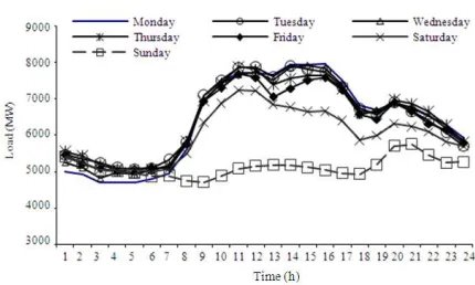
Fig. 2: Typical weekly load pattern

Special holidays such as Hari Raya Puasa (HRP), Independence Day (ID), Depavali (DPV), Chinese New Year (CNY), Christmas Day (CHM), Labor Day (LAB) and other special holidays all have the effect of lowering maximum load demand. For hourly load, the load pattern follows the activities of the consumers with the load demand increases steadily from 9 am to 12 noon with small decrease during midday and picks up again until 4 pm in the afternoon.

The customer’s behavior pattern can be described as follows-the demand decreases steadily after 4 pm until 7pm and increase again around 8-9 pm. The load demand decreases gradually to the lowest load demand in the early morning. The line graphs show that Sunday has the lowest load with Saturday the next lowest and for most of the rest of the days the load variation are rather small. In order to capture these two factors, a qualitative variable “day of the week” was introduced into the model through the specification of six dummy variables (Dit) representing all days in a week (Tuesday,

Wednesday, Thursday, Friday, Saturday and Sunday):

it

1 , t T u es , ..., S u n d ay D

0 , o th erw ise

=



= 

 (2)

The load demand decreases during holidays. For the model to take the decrease in demand into account, we introduced three additional dummy variables, first, the variable Hjt where j refers to priority level given by

different type of holidays. The priority values were chosen arbitrarily between [0,1] and were selected according to average load reduction values. Priority level one is assigned to CNY and HRP as these two holidays have the highest load reduction and also the longest duration of holidays. These holidays were given the highest weight reduction of one.

The second category is assigned to the next highest load reduction with priority level two which include HRP, LAB, ID, CHM and DPV. These are federal

holidays and major religious events. We set the priority value as 0.75 for load reduction weight. The monthly seasonality effect is observed by the inclusion of eleven dummy variables (Mjt), each representing one of the

months in a year with January as the base month. Thus, j begins with February and Mjt equals 1 if in the t

observation the month j is found and Mjt equals 0

otherwise:

jt

1, if j Feb, March,..., December. M

0, otherwise

for t 1, 2, , n

= =



= …

Regression time series is used to forecast time series that are deterministic in nature. Such models are useful when the parameters describing a time series are not changing over time. For such model, error term is assumed to be a random variable and statistically independent. However, when we employ time series regression, the residual sample autocorrelation and residual sample partial autocorrelation will indicate that the error terms are not statistically independent. The normal practice to overcome this problem is to model the error term using Box-Jenkins model. Combining the time series regression model with Box-Jenkins model and conducting a stepwise scheme starting with the simplest model, adding each time new terms in order to assess separately the effect of the different factors that influence the daily electricity demand and taking into account all the commented effects, the estimated model is finally given as:

t 1 1 max 1 max

7 12

1i it 1 t 1 1i jt 1t

i 2 j 2

L c t Temp Temp

D H+ M e

= =

= + α + β + γ

+

∑

∑

Where:

t = Time variable

βi: i = 1,2,..,k = Coefficients to be estimated for the

terms considering the different effects et = The residual term

1622 January and this implies that all the other months have higher electricity consumption compared to January except for February which has a lower electricity demand. On average, the month of January has lower electricity demand due to end of the year effect. The daily seasonality shows that Tuesday and Thursday are not significantly different from the base day, Monday. The coefficient for Wednesday is positive and significant which means that Wednesday has a higher consumption compared to Monday. All coefficients for Friday, Saturday and Sunday are negative and significantly different from Monday. This can be attributed to the weekend effect. Friday has the lowest demand for weekdays.

All coefficients for the dummy variables related to holiday effects are negative and significant indicating large demand decrease due to holidays, coefficients for Ht-1 indicates that the momentum for holiday has started

earlier usually a day before the holiday and this momentum is carried forward even after a holiday as shown by the significance Ht-1 which measure a day

after the holiday effect. Usually this effect is true during major religious holidays like CNY, HRP, HRH and DPV. The excitement of holiday tradition which is strongly rooted in most Malaysian cause this before and after holiday’s effect. Model 3 has a good predictive power with R2 equals to 90.32%.

Fuzzy Rule-Based System (FRBS): FRBS is a popular computing framework based on the concepts of fuzzy set theory, fuzzy IF-THEN rules and fuzzy reasoning[9,11,13]. It has found successful applications in a wide variety fields such as automatic control, data classification, pattern recognition, decision making and analysis, expert systems, forecasting and many more. This study also examines the feasibility of rule-based forecasting, a procedure that applies forecasting expertise and domain knowledge to produce forecasts according to features of available data. We developed a rule base facility to make hourly forecasts for electricity load demand. The development of the rule-based drew upon protocol analyses of a few experts on forecasting of electricity demand and experts on a few practical forecasting methods at the local utility company[4]. This rule based approach, consisting of many rules with many cases, established from established weather pattern using features of time series. This study also includes the effect of end-user’s behavior pattern. The behavior patterns of the end-user are based on a few actual observations, which are divided into daily and annual weekly load profile. The annual weekly load profile is used to explain the general lifestyle throughout the year.

The development of rule bases has many benefits and these include automating some tasks associated with maintaining a complex body of knowledge and providing knowledge in an accessible and modifiable form[5]. Besides its usefulness in forecasting, knowledge in this form aids reasoning about forecasting; that is, the knowledge is useful both procedurally and declaratively. We tested the feasibility of rule-based forecasting as a procedure to forecast hourly load demand for the next day. To do this, we have to establish a set of reasonable rules. We do not presume that they are the best set of rules. First, features of the series are identified and rules are then applied to produce short-range forecasting models. A simple rule base given below follows the structure of the thousands other rules along with brief explanations. Considering just the weather factor, rules are built according to the temperature at current hour, temperature of previous day (morning), temperature of previous day (afternoon), the current day (morning), the current day (afternoon), the forecasted day (morning) and forecasted day (afternoon). Some of the weather properties are weather for previous hour-day, weather for current hour-day and so on may be described as follows:

“temperature of current hour: CTHL, CTHM, CTHH (low, intermediate, high); temperature of the previous day, morning @ 1100: PTML, PTMI, PTMH; temperature of the previous day, afternoon @ 1600: PTNL, PTNI, PTNH; temperature of the current day, morning @ 1100: CTML, CTMI, CTMH; temperature of the current day, afternoon @ 1600: CTNL, CTNI, CTNH; temperature of the forecasted day, ;morning @ 1100: FTML, FTMI, FTMH; temperature of the forecasted day, afternoon @ 1600: FTNL, FTNI, FTNH; weather for the previous hour-day: PWHR, PWHC, PWHS (rainy, cloudy, sunny); weather for the current hour-day: CWHR, CWHC, CWHS; weather for the forecasted hour-day: FWHR, FWHC, FWHS; day-of-week indicator: DY01, DY02, DY03, DY04, DY05, DY06, DY07; previous day half-hour: PH01, PH02,... PH48 (0030,… 2400); current day half-hour: CH01, CH02,... CH48; forecasted day half-hour: FH01, FH02,... FH48; previous day half-hour load: PL01, PL02,... PL48; current day half-hour load: CL01, CL02,... CL48; forecasted day half-hour load: FL01, Fl02,... FL48”

temperature-I and the high temperature H. For the weather condition such as the rainy weather -R, the cloudy weather-C and the sunny weather-S; else f is set at 1.

Suppose that we intend to forecast the load demand for Thursday, one day in a week starting from as early as 0500 in the morning, we consider the load profiles on Tuesday and Wednesday to explain the relationship between daily end-user lifestyle and electricity load demand on the next normal working day. Reference is made to Fig. 2, to explain the load profile based on Peninsular Malaysia end-user daily lifestyle in a quantitative and subjective manner. A sample rule-base model can be described as follows:

If the forecasted day of the week is Thursday and temperature of the current hour is HIGH and temperature of the current day @1100 is HIGH and temperature of the current day @1600 is HIGH and temperature of the previous day @1100 is HIGH and temperature of the previous day @1600 is INTERMEDIATE and temperature of the forecasted day @1100 is HIGH and temperature of the forecasted day @1600 is HIGH and weather of the current day-hour is SUNNY and weather of the previous day-hour is RAINY and weather of the forecasted day-hour is SUNNY and load demand of the current hour is HIGH and load demand of the current day-hour is HIGH and load demand of the previous day-hour is INTERMEDIATE then the load demand of the forecasted day-hour is HIGH.

Note that the actual load recorded on DY (04) at 0830 is 9852 MW. The absolute Percentage Error of 0.14% which is rather small. This analysis can be repeated with other rules and it can be found that the result is consistent.

RESULTS

Comparing the results for the ARIMA model approach, the SARIMA model gave a much better forecast accuracy for forecasting peak load demand. It demonstrated that SARIMA model has the ability to predict future values where ARIMA model absolutely failed. It recorded the lowest mean square error of 0.00184 (Table 1). The forecasting performance of SARIMA model for electricity load demand is very sensitive and has significant impact on the forecasting accuracy[15].

Table 1: Comparison result between ARIMA models for Malaysian electricity generated forecast

Models ARIMA (1, 1, 1) SARIMA12 (1, 1, 0)(1, 0, 1)

Converged Yes Yes

Error term

SSE 0.24913 0.13441 MSE 0.00337 0.00184

Parameter estimate

φ1 -0.39760 -0.57810

θ1 0.24252 -

Φ1 - 0.91075

Θ1 - 0.33655

Fig. 3: Weekly forecast

Figure 3, shows the result generated using time series regression model by combining many factors. Modification of the basic regression model and modeled it using Box-Jenkins auto regressive error has produced a satisfactory and adequate model with 2.41% forecasting error.

In this study we managed to quantify the effect of holidays by grouping the holidays with similar load reduction pattern together and searching the best weights reduction for the groups. In this case, the load reduction weights obtained are 1, 0.65, 0.37 and 0.07 were used in the time series regression model for forecasting load demand.

DISCUSSION

1624

Table 2: Comparison between the forecasted and actual load Load (MW)

--- Method 04:00 11:00 16:00 20:00 Day MD MA3 8046 11232 11499 10553 11579 ES 0.8 7967 10961 11309 10584 11444 FRBS R-based 8458 11450 11858 10892 11858 Actual 8379 11590 10892 10994 12023

Table 3: Calculated error for various forecasting methods Error (%)

--- Method 04:00 11:00 16:00 20:00 Day MD MA3 3.08 3.09 1.77 4.01 3.69 ES 0.8 3.84 5.43 3.39 3.73 4.82 FRBS R-based -3.76 1.21 -1.30 0.93 1.37

Our results only drew upon general domain knowledge and anticipate significant gains from using specific domain knowledge. Currently we only make judgments about many of the features while some of these judgments could be replaced by mathematical and statistical procedures.

Table 2 shows that the load profiles generated by the Moving Average lag 3 and the ES 0.8 are consistently lower than the actual load demand throughout the day. However, the R-Based method produced a more similar load profile to the actual data. This can be confirmed by comparing the Mean Absolute Percentage Error computed for the rule-based method for the day is only 1.21% (Table 3). Comparing the peaks of the day, it is observed that the rule-based method also gives the most accurate forecast for these hours. The calculated errors at these ‘check-points’ are all within ±1.5% with exception of 0400 in the morning (Table 2).

CONCLUSION

With rule-based based forecasting, one can apply expertise about forecasting methods and domain knowledge that is appropriate to the conditions of time series. Prior literature suggests that such an approach should improve the accuracy of extrapolation forecasts under certain conditions. Rule-based forecasting was also more accurate than the standard moving average and exponential smoothing method. These improvements in accuracy base on MAPE were statistically significant[7]. In general, the improvement will depend on the conditions of the data, the knowledge development and validation. The rule-based forecasting procedure offers ideas to further study in this field. Hopefully, future study will be explored with fewer rules in order to achieve the better result.

ACKNOWLEDGEMENT

This research was supported by the Ministry of Science, Technology and Innovation, Malaysia (MOSTI) under IRPA Grant Vot No. 74285 and the Department of Mathematics, Faculty of Science, University Technology Malaysia. These supports are gratefully acknowledged. The authors would like to thank lecturers and friends for the helpful ideas and discussion. We also wish to thank Tenaga National Berhad for providing necessary data in this study.

REFERENCES

1. Collopy, F. and J.S. Armstrong, 1989. Toward computer-aided forecasting systems. Proceeding of the 9th International Conference on Decision Support System, (DSS’89), Institute of Management Science, pp: 103-119. http://works.bepress.com/j_scott_armstrong/9/ 2. Bunn, D. and G. Wright, 1991. Interaction of

judgmental and statistical forecasting methods: Issues and analysis. Manage. Sci., 37: 501-518. http://www.jstor.org/stable/2632457

3. Bowerman, B.L. and R.T. O’Connell, 1979. Forecasting and Time Series. Belmont, Duxbury Press, California.

4. Ismail, Z. and F. Jamaluddin, 2008. A backpropagation method for forecasting electricity load demand. J. Applied Sci., 8: 2428-2434. http://scialert.net/qredirect.php?doi=jas.2008.2428. 2434&linkid=pdf

5. Owayedh, M.S., A.A. Al-Bassam and Z.R. Khan, 2000. Identification of temperature and social events effects on weekly demand behavior. Proceeding of the IEEEPower Engineering Society Summer Meeting, July 16-20, IEEE Xplore Press, Seattle, WA., USA., pp: 2397-2404. DOI: 10.1109/PESS.2000.867364

6. Allison, P.D., 1999. Multiple Regression: A Primer. Thousand Oaks, Pine Forge Press, Inc., California, ISBN:0761985336, pp: 202.

7. Mohamad, N., M.H. Ahmad, Z. Ismail and K.A. Arshad, 2008. Multilayer feedforward neural network model and boz jenkins model for seasonal load forecasting. Ultra Sci., 20: 767-772.

8. Armstrong, J.S., 1988. Research needs in forecasting. Int. J. Forecast., 4: 449-465. http://papers.ssrn.com/sol3/papers.cfm?abstract_id =1172728

10. Zadeh, L.A., 1968. Fuzzy algorithm. Inform. Control, 12: 94-102.

11. Zuhaimy Ismail and Maizah Hura Ahmad, 2003. Delphi improves sales forecasts: Malaysia’s electronic companies experience. J. Bus. Forecast.,

22: 22-30.

http://direct.bl.uk/bld/PlaceOrder.do?UIN=135990 310&ETOC=RN&from=searchengine

12. Zaheeruddin and V.K. Jain, 2008. An expert system for predicting the effects of speech interference due to noise pollution on humans using fuzzy approach. Expert Syst. Appli., 35: 1978-1988

http://portal.acm.org/citation.cfm?id=1401468 13. Aznarte, M.J.L., J.M.B. Sanchez, D.N. Lugilde,

C.D.L. Fernandez and C.D. De La Guardia et al., 2007. Forecasting airborne pollen concentration time series with neural and neuro-fuzzy models. Expert Syst. Appli., 32: 1218-1225. http://portal.acm.org/citation.cfm?id=1222791

14. Kleinbaum, D.G., L.L. Kupper and K.E. Muller, 1998. Applied Regression Analysis and Other Multivariable Methods. 2nd Edn., PWS-KENT Publishing Company, Boston, ISBN: 10: 0534209106, pp: 798.

15. Makridakis, S. and M. Hibon, 1979. Accuracy of forecasting: An empirical investigation. J. R. Stat.

Soc. Ser. A., 142: 97-145.

http://www.jstor.org/stable/2345077

16. Makridakis, S., S.C. Wheelwright and R.J. Hyndman, 1998. Forecasting: Methods and Applications. 3rd Edn., John Wiley and Sons, Inc., New York, ISBN: 0471532339, pp: 656.