Journal of Symbolic Computation 43 (2008) 359–376
Symbolic Computation
Approximate Factorization of Multivariate Polynomials
Using Singular Value Decomposition
Erich Kaltofen
a
, John P. May
b,1
, Zhengfeng Yang
c
, Lihong Zhi
c
aDept. of Mathematics, North Carolina State University, Raleigh, North Carolina, 27695-8205, USA
bSchool of Computer Science, University of Waterloo, Waterloo, Ontario Canada
cKey Lab of Mathematics Mechanization, AMSS, Beijing 100080, China
Submitted 13 January 2006; revised received 18 April 2007; accepted 19 November 2007
Abstract
We describe the design, implementation and experimental evaluation of new algorithms for computing the approximate factorization of multivariate polynomials with complex coefficients that contain numeri-cal noise. Our algorithms are based on a generalization of the differential forms introduced by W. Ruppert and S. Gao to many variables, and use singular value decomposition or structured total least squares ap-proximation and Gauss-Newton optimization to numerically compute the approximate multivariate factors. We demonstrate on a large set of benchmark polynomials that our algorithms efficiently yield approximate factorizations within the coefficient noise even when the relative error in the input is substantial (10−3).
Key words: multivariate polynomial factorization, approximate factorization, singular value decomposition, numerical algebra, Gauss-Newton optimization
1. Introduction
When the scalars in the inputs to a symbolic computation are given as floating point num-bers, often with added noise that may come as the result of a preceding numerical computation or a physical measurement, the desired singular properties of the problem formulations can be lost. We shall consider the problem of factoring a multivariate polynomial into its complex fac-tors. Let f(x1, . . . ,xn)∈Q(i)[x1, . . . ,xn]be irreducible overC, where irreducibility is caused by
Email addresses:[email protected](Erich Kaltofen),[email protected](John P. May),
[email protected](Zhengfeng Yang),[email protected](Lihong Zhi).
1 Tel.: +1 519 747 2373; fax: +1 519 747 5284.
perturbations on the coefficients of f . By f[min] we denote a factorizable polynomial over C
with deg(f[min])≤deg(f)such thatkf−f[min]k2 is minimized, that is, f[min]is a nearest re-ducible polynomial. We present new algorithms that can find a factorization ef =f1·f2···frin
C[x1, . . . ,xn]with deg(ef)≤deg(f)such thatkef−f[min]k2is small.
In (Kaltofen and May,2003, Example 2) it was discovered that f[min]is dependent on the degree notion. Our bounds such as deg(ef)≤deg(f)limit the degrees in the individual vari-ables, that is degx
i(f˜)≤degxi(f)for i=1, . . . ,n. One of the authors, L. Zhi, had in Nov. 2002 considered to apply S. Gao’s exact polynomial factoring algorithm (seeGao,2003) for numer-ical coefficients. Independently, in the conclusion of (Kaltofen and May,2003) we have sug-gested that structural minimal deformations that achieve the necessary rank deficiency of the Ruppert matrices arising in S. Gao’s (2003) algorithm yield an approximate factorization al-gorithm. In (Gao et al., 2004) we have jointly designed and implemented a hybrid symbolic-numeric variant of Gao’s bivariate polynomial factoring algorithm. Our algorithm computes an unstructured singular value decomposition followed by a newly designed approximate bivariate greatest common divisor algorithm. Here we present a multivariate generalization and, following (Zeng and Dayton,2004), we introduce Gauss-Newton post-iteration, which can significantly improve the accuracy of the approximate factorization. As an alternative, one can use a struc-tured total least squares deformation (Park et al.,1999;Lemmerling et al.,2000) of the Ruppert matrices, which we demonstrate to be a feasible approach.
We present experimental evidence that our new approach improves the approximate factor-izations of (Gao et al., 2004). The difficulty of a satisfying numerical analysis of any of our algorithms are the notions of “near” and “small”. Our experiments show that our algorithms perform well even for polynomials with a relatively large irreducibility radius (Nagasaka,2002; Kaltofen and May,2003;Nagasaka,2005).
There is an extensive literature on the problem of factoring multivariate polynomials over the real or complex numbers. In (Kaltofen,1985) one of the first polynomial-time algorithms is given for input polynomials with exact rational or algebraic number coefficients, and the problem of approximate factorization is already discussed there (Kaltofen,1985, section 6). Approximate factorization algorithms suppose that the input coefficients are perturbed and consequently, the input polynomial is irreducible over Cunder an exact interpretation of its coefficients. How-ever, if the input polynomial is near its factorizable counterpart, say within machine floating point precision, one can attempt to run exact methods with floating point arithmetic, such as Hensel lifting, computing zero-sum relations of power series roots, or interpolating the irre-ducible factors as curves. The work reported in (Sasaki et al., 1991, 1992; Galligo and Watt, 1997;Huang et al.,2000;Sasaki,2001;Galligo and Rupprecht,2001;Corless et al.,2001,2002; Galligo and Rupprecht,2002;Rupprecht,2004;Sommese et al.,2004) studies recovery of ap-proximate factorization from the numerical intermediate results. For significant noise, which is the setting we study, those methods can suffer from stability problems. For instance, the approx-imate zero sums are now far from zero. A somewhat related topic are algorithms that obtain the exact factorization of an exact input polynomial by use of floating point arithmetic in a practically efficient way (Ch`eze,2004).
A different line of methods bounds from below the distance from the input polynomial to the nearest factorizable polynomial, that is, the irreducibility radius (Nagasaka,2002;Kaltofen and May, 2003; Nagasaka, 2005). Not only do such bounds help in declaring inputs numerically irre-ducible, they also provide insight in the quality of a computed approximate factorization.
al-gorithm is given for computing the nearest polynomial with a complex factor of constant degree. In practice, that algorithm is much slower than any of the numerical solutions—and the same may be expected of a future solution to the open problem—but for polynomials of degree 2 or 3 one can obtain an actual optimal answer with which one can further gauge the output of the fast but non-optimal numerical procedures.
With the algorithms presented in this paper, we have successfully computed improved approx-imate factorizations of all benchmark examples presented in the literature, including those with significant irreducibility radii introduced in (Gao et al.,2004).
2. Approximate Multivariate Polynomial Division and GCD
Our algorithms require, as a substep, the computation of approximate multivariate greatest common divisors of complex polynomials. Several of the algorithms available for approximate GCD further require an algorithm to compute approximate multivariate polynomial division, which we shall discuss first.
2.1. Approximate Polynomial Division
The simplest interesting problem in approximate polynomial algebra seems to be the problem of polynomial “exact” division. Multiplication by a given polynomial is a linear operation so we can represent multiplication of polynomials of total degree d by a given f as C[d](f), the convolution matrix associated with f and d. For instance,
−−−−−−−−−−−−−−−−−−−−−−−→
(a2x+a1y+a0)·(b2x+b1y+b0) =C[2](a2x+a1y+a0)·
b2 b1 b0 =
a2 0 0 a1 a2 0 0 a1 0 a0 0 a2
0 a0 a1 0 0 a0
· b2 b1 b0 .
Note that the convolution matrix can be formed for other notions of degree (or polynomials with a given support), but for simplicity of discussion we will use total degree in our descriptions in this section. The results carry over to all degree notions.
If we are given polynomials f and g with tdeg(g)≥tdeg(f)such that f does not divide g exactly then we want to apply a perturbation so that f does divide g. If we fix the coefficients of f then ˜g, the closest polynomial to g that f divides, can be found by solving the least squares problem:
min
tdeg(q)=tdeg(g)−tdeg(f)kf q−gk2. (1) We can write ˜g exactly in terms of a convolution matrix,
˜
(where we are being intentionally sloppy about the distinction between g as a polynomial and g as a vector of its coefficients). In the univariate case, the coefficient matrix for the least squares problem (1) has a small displacement rank and the arising system can be solved efficiently (Zhi, 2003).
One of the shortcomings of this approach is, although it does solve the approximation problem completely, it does not allow for f to vary as well (or instead of) g. However, it is very easy to implement, and the results it provides seem good enough for our purposes.
If one wished to allow perturbations of the coefficients of both f and g, then the division problem becomes a total least squares (TLS) problem (perturbations are allowed in the right-hand side vector as well as the entries of the matrix). In fact, since the matrix C[d](f)has a very specific structure, approximate division becomes a structured total least squares (STLS) problem. 2.2. Approximate Polynomial GCD
For completeness we restate the algorithm in (Gao et al.,2004). A very similar multivariate approximate GCD algorithm was proposed independently in (Zeng and Dayton,2004) but a pre-specified toleranceεis required there. In addition, a Gauss-Newton iteration step is introduced to improve the GCD further. In practice just a few steps of iteration can improve the backward error by at least an order of magnitude and so it is usually worth the extra computation, especially when the g and h started quite close to a pair with a non-trivial GCD. For example, if g and h are nearly machine precision distance from a pair with an exact GCD, the approximate GCD computed from the SVD method is generally limited to about half of the machine precision, while Gauss-Newton iteration can usually improve the result to exact within full machine precision. Algorithm 1 (AMVGCD: Approximate Multivariate GCD).
INPUT: g and h inC[x1, . . . ,xn]
OUTPUT: d, a non-constant approximate GCD of g and h
(1) Determine k, the degree of the approximate GCD of g and h, in one of the two ways below: (a) Form S=S1(g,h), the matrix of the linear system ug+vh=0, where g,h∈C[x1, . . . ,xn]
with tdeg(u)<tdeg(h)and tdeg(v)<tdeg(g). Find the largest gap in the singular val-ues of S and infer the degree from the numerical rank of S.
(b) Compute the degrees of the GCDs of several random univariate projections of g and h by looking for the numerical rank of the corresponding univariate Sylvester matrices. (2) Reform S as Sk(g,h)that is, use tdeg(u) =tdeg(h)−k and tdeg(v) =tdeg(g)−k as the
constraints on u and v in the linear system in the first step. This new S will have a dimension 1 nullspace.
(3) Compute a basis for the nullspace of S by computing the singular vector corresponding the smallest singular value of S. This vector gives a solution[u,v]T.
(4) Find d, the approximate quotient of h and u (or g and v); alternately minimizekh−d uk22+
kg+d vk22, using least squares.
If one wishes to specify a tolerance, then only the first step of the Algorithm1is affected. In that case, it is possible that the computation of the degree could yield k=0, in which case the method would return d=1, declaring g and h to be approximately relatively prime to the given tolerance.
2006).
3. The Factorization Algorithm and Experiments
In this section, we propose an approximate factoring algorithm for multivariate polynomials overC. The algorithm is a generalization of the bivariate factoring algorithm in (Gao et al.,2004). In addition, we have incorporated Gauss-Newton post-refinement of the approximate factors. Much like the GCD algorithm presented above, our factoring algorithm relies on singular value decomposition. We have implemented our algorithm in Maple 10 and we present benchmark tests.
3.1. The Exact Factoring Algorithm
We briefly describe the multivariate generalization of the bivariate factoring algorithm in (Gao, 2003), more details can be found in (May,2005).
Assume that f is non-constant and gcd(f,fx1) =1 where fx1 =∂f/∂x1, which makes f both
square-free and with no factor inC[x2, . . . ,xn]. Suppose that f factors as
f= f1f2···fr, (2)
where fi∈C[x1,x2, . . . ,xn]are distinct and irreducible overC. Define
Ei=
f fi
∂fi
∂x1∈
C[x1,x2, . . . ,xn]1≤i≤r. (3)
Then
fx1 =E1+E2+···+Erand EiEj≡0 mod f for all i6=j. (4)
The following fact, for two variables stated first in (Ruppert,1986), gives a test for irreducibil-ity and is a key part of the factoring algorithm.
Fact 2. Suppose f ∈C[x1,x2, . . . ,xn]with multi-degree(d1,d2, . . . ,dn), i.e., degxif =di. Then f is absolutely irreducible if and only if the equations
∂ ∂xi
µg
f
¶
= ∂
∂x1
µh
i
f
¶
,i=2, . . . ,n (5)
have no nonzero solution g,h2, . . . ,hn∈C[x1,x2, . . . ,xn]with
deg g ≤(d1−2,d2, . . . ,dn),
deg hi ≤(d1,d2, . . . ,di−1, . . . ,dn),i=2, . . . ,n.
(6)
Since differentiation is linear over C, the equations (5) give a linear system for the coef-ficients of g and hi, whose coefficient matrix we call the Ruppert matrix Rup(f). The
First, let us note that, similar to (Gao,2003) and (Kaltofen and May,2003), the degree condi-tions on g and the hiare changed to:
deg g ≤(d1−1,d2, . . . ,dn),
deg hi ≤(d1,d2, . . . ,di−1, . . . ,dn),i=2, . . . ,n,
(7)
which allows for the solution(fx1,fx2, . . . ,fxn)even when f is irreducible. We use Rup1(f)to denote the slightly larger coefficient matrix of (5) using the bounds (7).
Theorem 3. Let f∈C[x1,x2, . . . ,xn]be a non-constant polynomial of multi-degree(d1,d2, . . . ,dn)
with gcd(f,fx1) =1. Define
G={g∈C[x1,x2, . . . ,xn]:(5)and (7) hold for some h2, . . . ,hn∈C[x1,x2, . . . ,xn]} (8)
Suppose f has the factorization into irreducible polynomials as in (2). Then G is a vector space overCof dimension r and each g∈G is of the form g=∑r
i=1λiEiwhereλi∈C.
The proof that follows is a direct multivariate generalization ofGao(2003, Theorem 2.3). First, for any gk=Ek= ff
k
∂fk
∂x1, let hk,i=
f fk
∂fk
∂xi, for i=2, . . . ,n. Then(gk,hk,2, . . . ,hk,n)satisfies (7) and
∂ ∂xi
µ
gk
f
¶
= ∂
∂xi
µ
1 fk
∂fk
∂x1
¶
= ∂
∂x1
µ
1 fk
∂fk
∂xi
¶
= ∂
∂x1
µ
hk,i
f
¶
,
for i=2, . . . ,n.So E1, . . . ,Er∈G. Since E1, . . . ,Ersatisfy (4), they are linearly independent over
C. Hence dimCG≥r.
Let g∈G with h2, . . . ,hn∈C[x1,x2, . . . ,xn]satisfying (5) and (7). We need to show that g is
a linear combination of E1, . . . ,EroverC. Since gcd(f,fx1) =1, f has no repeated roots in the
algebraic closure ofC(x2, . . . ,xn). Let
f=ud1
d1
∏
i=1
(x1−ci),ci∈C(x2, . . . ,xn).
Due to degx
1g<degx1 f and degx1hj≤degx1 f , we have the partial fraction decompositions g
f =
d1
∑
i=1 ai
x1−ci
, hj f =
d1
∑
i=1 bji
x1−ci
+h∗j,
where bji∈C(x2, . . . ,xn), degx1h ∗
j=0,
ai=g(ci,x2, . . . ,xn)/fx1(ci,x2, . . . ,xn). (9)
Since
∂ ∂xj
µg f ¶ = d1
∑
i=1
µ 1
x1−ci
∂ai
∂xj
+ ai (x1−ci)2
∂ci
∂xj
¶
, ∂
∂x1
µh j f ¶ = d1
∑
i=1
−bji
(x1−ci)2
.
The equation (5) implies that ∂ai
they are inC. Therefore aiis constant for ciin the same conjugate class which corresponds to an
irreducible factor of f overC(x2, . . . ,xn). So as in (Gao,2003), we have that
g f =
r
∑
i=1
λi
1 fi
∂fi
∂x1 ,
whereλi∈C. Therefore, each g∈G is of the form g=∑ri=1λiEiand dimCG=r. 2 Now we show how to extract the factors of f from the linear space G. This is the direct generalization ofGao(2003, Theorems 2.9 and 2.10):
Fact 4. Suppose that g1, . . . ,gr form a basis for G overC. Select si∈S⊂Cuniform randomly
and independently for all 1≤i≤r, and let g=∑r
i=1sigi. There is a unique r×r matrix A= [ai,j]
overCsuch that
ggi≡ r
∑
j=1
ai,jgjfx1 (mod f) inC(x2, . . . ,xn)[x1]. (10)
Furthermore, let Eg(x) =det(Ix−A), the characteristic polynomial of A. Then the probability
that
f=
∏
λ∈C: Eg(λ)=0
gcd(f,g−λfx1) (11)
gives a complete factorization of f overCis at least 1−r(r−1)/(2|S|), where|S|denotes the cardinality of S.
Again, the proof is nearly exactly the same as the one in (Gao,2003).
It is possible to reduce Gao’s degree conditions (7) to Ruppert’s (6) in the factoring algorithms. For completeness, we state the corresponding theorem, whose proof reveals how to modify the factoring algorithms.
Theorem 5. Let gcd(f,fx1) =1. Then Rup(f)has rank deficiency r−1, i.e., the dimension of the nullspace of Rup(f)is r−1, where r is the number of irreducible factors of f overC.
The proof is based on Ruppert’s original arguments (Ruppert,1999, Section 3). Clearly, any solution g,h2, . . . ,hnof Theorem3that satisfies the stricter bound (6) corresponds to a vector in
the nullspace of Rup(f). For k=2, . . . ,r the polynomials degx
1(fk)g1−degx1(f1)gk
| {z }
ˆ gk
,degx
1(fk)h1,2−degx1(f1)hk,2,
. . . ,degx1(fk)h1,n−degx1(f1)hk,n,
where gkand hk,iare as in the proof of Theorem3, are such solutions, i.e., degx1(gˆk)≤d1−2,
be-cause the leading coefficients in the variable x1of degx1(fk)g1=degx1(fk)
f f1
∂f1
∂x1 and degx1(f1)gk=
degx
1(f1)
f fk
∂fk
∂x1 cancel. The corresponding coefficients vectors are linearly independent, so the
coefficient vectors, but the solution g=∂f/∂x1, h2=∂f/∂x2, . . . ,hn=∂f/∂xnfor Rup1(f)is
not in that span, since the degree in x1of g is too high. 2
The following paragraph is omitted from the journal version.
Now suppose we have computed polynomials v2, . . . ,vr whose coefficient vectors form a basis
for the g-component of the nullspace of Rup(f). By basis transformation we have vj=∑kµj,kgˆk
for j=2, . . . ,r, where[µj,k]∈C(r−1)×(r−1)is non-singular. Therefore
∑
j
sjvj=
∑
k(
∑
j
sjµj,k)gˆk
=³
∑
k
degx
1(fk)
∑
j
sjµj,k
´
| {z }
λ1(s2, . . . ,sk)
g1−
∑
k
³
degx
1(f1)
∑
j
sjµj,k
´
| {z }
λk(s2, . . . ,sk)
gk
For symbolic sj we have∏i<l(λi(s2, . . . ,sk)−λl(s2, . . . ,sk))6=0, because the columns of[µj,k]
are linearly independent. Note that the coefficient of sjconstitutes the j-th row of those columns.
By Zippel/Schwartz∑jsjvjhas distinctλiwith probability(r−1)(r−2)/(2|B|).
End of material omitted from the journal version. c°authors.
3.2. The Numerical Factoring Algorithm
In order to apply the factorization algorithm given in (Gao,2003) and its multivariate gen-eralization, given above, to approximate polynomials we must be able to solve the following problems:
(1) compute the approximate GCDs of multivariate polynomials: gcd(f,g−λifx1),
(2) reduce the polynomial f so that gcd(f,fx1) =1 approximately,
(3) determine the numerical dimension of G, and (4) compute an Egthat has no cluster of roots.
For the first problem, the previous section discusses robust algorithms to compute the approx-imate GCDs of multivariate polynomials. The second problem is also handled by way of the approximate GCD; we can compute the approximate GCD of f and fx1. Then with an
approx-imate division, f/gcd(f,fx1), we may, heuristically, reduce to the case where gcd(f,fx1) =1
approximately. Details on this approach follow below in Section3.4.
To solve the third problem we can determine the numerical dimension of G by the SVD of the matrix Rup1(f). Letσi be the ithsingular value of Rup1(f). If a toleranceε is given, then the numerical dimension of G is the r such that
··· ≥σr+2≥σr+1>ε≥σr≥ ··· ≥σ1.
However, if we do not know the relative error in the coefficients of f , it is difficult to provide a toleranceεthat is consistent with the error in the data. If we have no tolerance given, we infer a tolerance from the largest gap in the singular values. That is, we chooseε=σrso thatσr+1/σr
is as large as possible. As in (Kaltofen and May,2003), the singular valueσrbounds from below
the distance from f to a polynomial ˜f that has r absolutely irreducible factors: min
deg ˜f=(d1,...,dn) dim Nullspace(Rup1(f˜))=r
This inferred toleranceσrcan also be used as an input tolerance to the approximate multivariate
GCDs at the end of the factorization algorithm.
Remark 6. Ideally, we could apply a structure preserving low rank approximation (SPLRA) as in (Park et al.,1999) to obtain a matrix ˜R which is closest to Rup1(f)and has rank deficiency r. Since ˜R preserves structure of Rup1(f), it corresponds to the Ruppert matrix of a polynomial
˜
f which is the nearest polynomial that has exactly r absolutely irreducible factors. However, so far our experiments with applying various heuristics for SPLRA to this problem have had mixed results. So we leave details of research in this direction to be reported in future papers. In the following, we still use the SVD of the Rup1(f)to find a nearby rank deficient matrix.
For the fourth problem, suppose we have obtained approximate basis g1, . . . ,gr of G from
the singular vectors corresponding to the last r singular values of Rup1(f). It is easy to see that kRup1(f)gik2≤σi≤σr. So the gis form an approximate basis for G with tolerance σr.
Following construction of the matrix Agas described in Fact4, we find a random element of G
by choosing s1, . . . ,sr∈S⊂Cuniform randomly, letting g=∑ri=1sigiand substituting arbitrary
values ofαi∈Cfor xiwith the property that f(x1,α1, . . . ,αn−1)remains square-free. The matrix Agcan be formed in the following manner: first reduce the polynomials ggiand gjfx1 modulo f
(evaluated at xk=αk) for 1≤i,j≤r by using approximate division of univariate polynomials
(see Section2.1) then solve the least squares problem: minkrem(ggi−(ai,1g1fx1+···+ai,rgrfx1), f)k2
to find the value of unknown elements ai,j. Let Eg(λ) =det(Iλ−A), the characteristic
polyno-mial of Ag. We compute all the numerical rootsλ1, . . . ,λr of the univariate polynomial Egover
Cas the eigenvalues of Ag, and find the smallest distance between these roots:
min dist(g) =min{|λi−λj|, 1≤i<j≤r}.
If the distance is small then numerically Eghas a cluster of roots, and we should choose another
set of sis and try to find a separable Eg. In practice, since Fact4says g should give a separable
Egwith high probability, we compute a number of random gs and keep the g with the largest
min dist(g).
In Gao’s exact algorithm the absolutely irreducible factors are obtained from g by computing GCDs over algebraic extension fields given by the irreducible factors of Eg. In our case, all
the roots of Egare given as numerical values inC. Hence there is no need to deal with field
extensions, and we can compute directly inC. We compute the multivariate approximate GCDs ˜
fi=gcd(f,g−λifx1)according to the method in Section2for each numerical rootλiof Egand
we obtain a proper approximate factorization of f overC: f ≈∏ri=1f˜i.
Once we have computed an approximate factorization, there are a number of ways to improve it. First, we can compute a scaling c that minimizes the backward error of the approximate fac-torization:
min
c∈Ckf−c
r
∏
i=1 ˜
fik2/kfk2.
(Zeng and Dayton,2004). First note that the optimization version of the approximate factoriza-tion problem is finding a least squares solufactoriza-tion to the non-linear system of the form F(v1, . . . ,vr) =
f where vi∈C[x1, . . . ,xn]and
F(v1, . . . ,vr) =
h
C[tdeg(v2···vr)](v
1)···C[tdeg(vr)](vr−1)vr
i
.
Here C[k](v)denotes the matrix of the linear map multiplication with polynomials of total de-gree k as described in subsection2.1. Clearly there is a solution when f =f1···fr and vi= fi;
otherwise we will solve min
v1,...,vrk
F(v1, . . . ,vr)−fk2.
There exists such a minimum at one or more of the points where (DF(v1, . . . ,vr))HF(v1, . . . ,vr) =0
(DF denotes the Jacobian of F). When formulated this way, it is easy to see that we can apply Gauss-Newton iteration to attempt to find the solution. That is, given an initial[v01,v02, . . . ,v0r]we refine with the update
[vi1+1, . . . ,vri+1] = [vi1, . . . ,vri]−(DF(vi1, . . . ,vir))†F(vi
1, . . . ,vir).
Given the description of F above, the product rule gives that the Jacobian of F is a block matrix of the form:
DF(v1, . . . ,vr) = [C[tdeg(v1)](v2v3···vr)C[tdeg(v2)](v1v3···vr). . .C[tdeg(vr)](v1v2···vr−1)]
which has full rank (so long as not all the vi’s are 0) since every matrix C[k](v)has full rank (so
long as v6=0).
As with any type of Newton method, if the initial input [v0
1,v02, . . . ,v0r] is close enough and
DF is not rank deficient at the least squares solution, then the iteration will converge to the least squares solution according toKelley(1999, Theorem 2.4.1):
Fact 7. Let w0= [v01, . . . ,v0r]be the initial point and w⋆= [v⋆1, . . . ,v⋆r]be a local minimum for F.
If DF is full rank then there exist K>0 andδ>0 so that ifkw0−w⋆k<δ then the error of the Gauss-Newton iteration update at step k (ek) satisfies:
kekk2<K(kek−1k22+kF(w⋆)−fk2kek−1k2).
3.3. Algorithm
Algorithm 8 (AFMP: Approx. Factoring Multivariate Polynomials).
INPUT: A polynomial f∈C[x1, . . . ,xn]such that f and fx1 are approximately relatively prime,
that is f is approximately square-free and has no approximate factors inC[x2, . . . ,xn](see
Sec-tion3.4below).
OUTPUT: A list of approximate factors fiand an optimal scaling c.
Let S be a finite set S⊂Cwith|S| ≥tdeg(f)2. In our implementation S={k/B| −B≤k≤B} for a size parameter B.
(1) Compute approximate nullspace solutions: (a) Form the matrix Rup1(f);
(b) Compute the singular value decomposition of the Ruppert matrix, and find the last tdeg(f) +1 singular valuesσi;
(c) Find the biggest gap in the singular values and decide the numerical dimension r of G, assuming r≥2;
(d) Form a basis g1, . . . ,grof G from the last r right singular vectors of Rup1(f). (2) Compute an Egwith well spaced roots:
(a) Evaluate at randomly selected values for the variables xi=αi that do not change the
degree or the square-free property of f ;
(b) For k from 1 to K do (K=4 seems to work well in practice) (i) Pick si,k∈S randomly, and set ¯gk=∑ri=1si,kgi
(ii) Compute ai,j,kthat minimize the norm of the univariate remainder:
minkrem(¯gkgi− r
∑
j=1
ai,j,kgjfx1, f)k2;
(iii) Let Eg¯k(x) =det(Ix−A), where[Ag¯k]i,j= [ai,j,k]. Compute the numerical rootsλi,k,1≤ i≤r of Eg¯k(the numerical eigenvalues of Ag¯k) and set min distk=min1≤i<j≤r{|λi,k−
λj,k|};
(c) Let g=g¯kwhere min distkis maximal.
(3) Compute factors via approximate GCDs:
Compute fi=gcd(f,g−λifx1)overC[x1, . . . ,xn]for 1≤i≤r.
(4) Solve optimizations to refine the factorization:
(a) Apply Gauss-Newton iteration to improve the approximate factors; (b) Compute minc∈Ckf−c∏ri=1fik2/kfk2.
Remark 9. Two aspects need to be clarified about the approximate GCD computation in step 3. First, in order to obtain the degree of the multivariate GCD, it is fastest to project to univariate problems using a toleranceεin Step 1 of Algorithm AMVGCD in Section2.2. The use ofσr
Remark 10. It is clear that output polynomials cannot be guaranteed to be approximately irre-ducible. For example, in the case that the input does not lie near a factorizable polynomial then the approximate GCDs may place a factor near a reducible polynomial. One may, of course, always achieve approximate irreducibility certification by applying the test given in (Kaltofen and May, 2003) (generalized to multivariate polynomials in (May,2005)) to the produced factors and apply the algorithm again if necessary.
Remark 11. The shape of the matrix Rup1(f)depends on the degree of f in each xi. Thus,
Algorithm8will find an approximate factorization of f which will have the same (or smaller) degree in each xibut one which may have higher total degree than f . If one wishes to find an
approximate factorization with the same total degree as f one can use a structured version of the Ruppert matrix that depends on the total degree of f . For more details see (May,2005, Section 3.2).
In the examples and implementation below, the total degree preserving version of the Ruppert matrix has been used. Product of the approximate factors found will always have total degree less than or equal to the the total degree of the original polynomial. Note that it is possible that the nearest polynomial that factors may have higher total degree. See (Kaltofen and May,2003) for details.
Remark 12. For the approximate algorithm, our choice of S is based on experimental success. In fact, we worked with B=10 with good results, requiring re-selection of ¯g2, . . .in Step (2.b.i) rarely.
3.4. Multiple Factors
In the case that f is quite close to a polynomial that is not square-free, our factorization algo-rithm does not work well. This is related to the fact that the exact algoalgo-rithm does not work at all on polynomials with repeated factors. In that case Rup1(f)has many extraneous null vectors that do not correlate with factors (at least, not in the same way). When an irreducible polynomial is near a repeated factor polynomial, the approximate null vectors and numerical rank of Rup1(f) exhibit some of these same problems. Another, similar but lesser problem is the removal of ap-proximate factors inC[x2, . . . ,xn], that essentially amounts to a multivariate approximate GCD
computation of several polynomials (Kaltofen et al.,2006).
One method to deal with the non-square-free case is to compute fsqfr, the approximate quo-tient of f and the approximate GCD of f and fx1 (Gao et al.,2004). Then compute the distinct
approximate factors of fsqfr≈ f1···fr using our algorithm. Finally, determine powers for each
factor by looking for gaps in the sequenceαi,j=σ1(S1(fi,∂x1,jf)).
We can only definitively call f approximately square-free if all of the nearest polynomials that factor are square-free. We cannot compute the nearest polynomial that factors, but we can bound the distance to the nearest polynomial that factors using the singular values of Rup1(f)as in (Kaltofen and May,2003), and similarly bound the distance to the nearest polynomial that is not square-free using the singular values of S1(f,fx1). If the two bounds are very close we have to
compute the factorization both ways and use the one with smaller backwards error.
3.5. A Factoring Example
We illustrate our algorithm by factoring the following noisy polynomial (from (Kaltofen, 2000)) over the complex numbers:
f :=81x4+72x2y2+0.002x2z2−648x2+16y4+0.001y2z2
−288y2+1296−648.003z4−0.007z2. The above polynomial is obtained by multiplying
(9x2+4y2+25.45596z2−36)(9x2+4y2−25.45578z2−36),
and rounding to three decimal places. Since deg f= (4,4,4), the Ruppert matrix (with respect to total degree) is 168×60. The last several singular values of the matrix are:
···,198.661,145.253,0.868×10−10,0.431×10−12.
Starting from the second smallest singular value, the biggest gap is 145.253/0.868×10−10=0.167×1013.
So r=2 and f is supposed to be close to a polynomial having two irreducible factors. A basis for G computed from the last two right singular vectors is:
g1=0.000151524784 x3−0.000606279 x+0.000067324 xy2+0.233157269 xz2, g2=0.108724346 x3−0.434897383 x+0.048321932 xy2−0.000322604 xz2.
Take a random linear combination of g=g1+g2and set y=2 and z=−1. A= [ai,j]can be
computed as
0.000336771 0.000192632 0.000335102 0.000335302
Two eigenvalues of the matrix A areλ1=0.000590107, λ2=0.000081966. Computing fi=
gcd(f,g−λifx), i=1,2, we obtain two factors of f :
f1=406.598 x2+180.710 y2−1150.03 z2−1626.39, f2=406.596 x2+180.709 y2+1150.04 z2−1626.39.
By finding an optimal scaling factor c=0.00048996 that minimizeskf−c f1f2k2we find the factorization:
√
c f1=9.000015518 x2+4.000009094 y2−25.45583592 z2−36.00004257,
√
c f2=8.999984448 x2+3.999990906 y2+25.45597017 z2−35.99995743,
that has a backward errorkf−c f1f2k2/kfk2=4.67×10−13. We apply Gauss-Newton iteration and find an improved factorization (rounded to 10 decimal places):
3.6. Implementation and Experiments
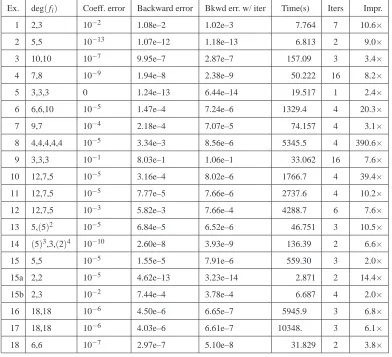
The AFMP algorithm and its variants have been implemented in Maple and tests are reported in (Gao et al.,2004). There, Gauss-Newton iteration was not used to improve approximate GCDs or the final factorization. Here we report the results of repeating the experiments with iterative improvement in Table1. Timings are given for some well known and some randomly generated examples run on a Pentium 4 at 2.0 GHz for Digits=14 in Maple 10 under Windows. Here coeff. error indicates the noise imposed on the input, namely the relative 2-norm coefficient error to the original product of polynomials. Both backward error and bkwd. err. w/ iter. are relative errors, namelykf−∏if˜ik2/kfk2. Please note that some incorrectly stated backward errors in (Gao et al.,2004) have been corrected here. The time is that for the entire factorization in seconds of a single run; the timings on a given example can vary significantly (up-to a factor of 4) depending on the random choices made in the algorithm; the Gauss-Newton iteration is generally less than 10% of the total time. The column iters is the number of Gauss-Newton iterations that were run before convergence – further iteration did not improve the factorization. Notice that the number of iterations increases as the backward error of the solution found increases (as discussed in the paragraph following Fact7). The column impr. indicates the factor by which the backwards error was improved by iterative refinement.
Our experiments seem to indicate that refinement will tend improve to backward error by about one order of magnitude over the results originally achieved in (Gao et al.,2004). The improve-ment can be quite a bit more pronounced if the original polynomial was within machine precision of being factorizable. In example 9, the factorization found before refinement had backward error worse than 2.37e-1, the backward error of the trivially factorizable polynomial f(x,y)−f(0,y), while that is beaten slightly after refinement. As can be seen by the number of iterations, when
knoisek ≈10−1it is still very difficult to get good results.
One can also compute the forward error of each factorization, by which we mean the relative 2-norm coefficient vector distance of a computed approximate factor to the nearest originally chosen factor, before noise was added to the product. For the examples our implementation pro-duced forward errors that are of the same magnitude of the stated backward errors, with the exception of Example 9 where the degrees of the produced approximate factors are 4 and 5, hence the forward error is, in some sense, infinite.
In Table1:
• Example 1 is from (Nagasaka,2002) where an approximate factorization with backward error 0.000753084 is also given (although this is slightly smaller than the backward error computed in the table and the given factorization does not seem to have been generated with any sort of general technique and no timing was reported2);
• Examples 2 and 3 are from (Sasaki,2001); Sasaki’s algorithm takes 430ms and 2080ms on a SPARC 5 (CPU: microSPARCΠ, 70 MHz) and produced backward errors of 10−9and 10−5, respectively;
• Example 4 is from (Corless et al.,2001); the backward error for their approximate factoriza-tion is reported as 0.47×10⁻⁴, compared to our backward error 2.38×10⁻⁹(no timings were reported);
• Example 5 is from (Corless et al.,2002), which is the factorization of an exact polynomial of
2 Note added January 22, 2008: this smaller backward error is possible because the perturbed polynomial has increased
Table 1
Algorithm performance on benchmarks
Ex. deg(fi) Coeff. error Backward error Bkwd err. w/ iter Time(s) Iters Impr.
1 2,3 10−2 1.08e–2 1.02e–3 7.764 7 10.6×
2 5,5 10−13 1.07e–12 1.18e–13 6.813 2 9.0×
3 10,10 10−7 9.95e–7 2.87e–7 157.09 3 3.4×
4 7,8 10−9 1.94e–8 2.38e–9 50.222 16 8.2×
5 3,3,3 0 1.24e–13 6.44e–14 19.517 1 2.4×
6 6,6,10 10−5 1.47e–4 7.24e–6 1329.4 4 20.3×
7 9,7 10−4 2.18e–4 7.07e–5 74.157 4 3.1×
8 4,4,4,4,4 10−5 3.34e–3 8.56e–6 5345.5 4 390.6×
9 3,3,3 10−1 8.03e–1 1.06e–1 33.062 16 7.6×
10 12,7,5 10−5 3.16e–4 8.02e–6 1766.7 4 39.4×
11 12,7,5 10−5 7.77e–5 7.66e–6 2737.6 4 10.2×
12 12,7,5 10−3 5.82e–3 7.66e–4 4288.7 6 7.6×
13 5,(5)2 10−5 6.84e–5 6.52e–6 46.751 3 10.5×
14 (5)3,3,(2)4 10−10 2.60e–8 3.93e–9 136.39 2 6.6×
15 5,5 10−5 1.55e–5 7.91e–6 559.30 3 2.0×
15a 2,2 10−5 4.62e–13 3.23e–14 2.871 2 14.4×
15b 2,3 10−2 7.44e–4 3.78e–4 6.687 4 2.0×
16 18,18 10−6 4.50e–6 6.65e–7 5945.9 3 6.8×
17 18,18 10−6 4.03e–6 6.61e–7 10348. 3 6.1×
18 6,6 10−7 2.97e–7 5.10e–8 31.829 2 3.8×
degree 9 (here their and our backward errors are about the same; no timings were reported);
• Examples 6 to 13 and 15 to 17 were constructed by choosing factors with random integer coefficients in the range−5≤c≤5 and then adding a perturbation; for noise we choose a relative tolerance 10−e, then randomly choose a polynomial that has the same degree as the
product, 25% as many terms (5% for Example 10 and 99% for Example 17) and coefficients in[−10e,10e]; finally, we scale the perturbation so that the relative error is 10−e;
• Examples 10, 11 and 12 approximately factorize the same polynomial with perturbations of different noise level and sparseness;
• Example 13 has repeated factors denoted with exponents in the degrees column; it should be noted that the improved factorization found by Gauss-Newton iteration still has a squared factor even though the refinement iteration does not treat the identical factors differently than non-identical factors.
• Example 15, 15a, and 15b are polynomials in three variables; 15a is from (Kaltofen,2000) and is worked in detail in Section3.5; Example 15b is from (Huang et al.,2000) where the backward error for their approximate factorization after refinement is reported as 5.72e-4;
• Example 18 is a polynomial with complex coefficients, where the real and imaginary parts of the coefficients of the factors were chosen random integers in[−5,5]. Noise was added to the real and imaginary parts of all terms.
The implementation reported in (Gao et al.,2004) also successfully found the approximate factors of four examples, provided by Jan Verschelde, which arise in the engineering of Stewart-Gough platforms (see (Sommese et al.,2004)). The input polynomials in 2 and 3 variables of degree 12 have small absolute coefficient error, 10−16, and have approximate factors of multi-plicities 1, 3 and 5. The trivariate approximate factors were computed via sparse numerical inter-polation using the techniques of (Giesbrecht et al.,2004,2006), (which is possible in this exam-ple because the forward error in the approximate factor coefficients is near machine precision). The running times, no more than 200 seconds with a backward error of no more than 7.62·10−9, appear much faster than what (Sommese et al.,2004) report for their solution, though this is part due to the advantage gained by using the sparse interpolation code reported in (Giesbrecht et al., 2004,2006).
The Maple implementation and benchmark runs can be found online at http://www.math.ncsu.edu/∼kaltofen/software/appfac/paper07 mws/ orhttp://www.mmrc.iss.ac.cn/∼lzhi/Research/hybrid/appfac/. 4. Concluding Remarks
Wolfang Ruppert’s differential forms (Ruppert, 1986, 1999) not only lead to a new exact factorization algorithm (Gao, 2003), they yield a formulation as a nearest structured singular matrix problem in the approximate setting. That setting then allows the application of sev-eral methods from numerical analysis, such as singular value decomposition (SVD), which has been already applied in the area of hybrid symbolic/numeric algorithms in (Corless et al.,1995; Emiris et al.,1997;Gianni et al.,1998;Zeng,2003). Here we have shown that the SVD-based approach followed by Gauss-Newton iteration can efficiently produce approximate factoriza-tion, which on our reversely engineered benchmark examples have a backward error as near as the introduced coefficient noise. Recently, structured least norm algorithms (Park et al.,1999; Lemmerling et al.,2000) have been successfully applied to hybrid symbolic/numeric algorithms (Kaltofen et al.,2007;Botting et al.,2005;Kaltofen et al.,2006) and we can report that they are a viable alternative to the SVD/Gauss-Newton approach.
For polynomials with many variables, the arising structured totals least norm problems have a very high dimension. One approach, already mentioned in section3.6, is to use sparse numerical interplolation (Giesbrecht et al.,2006) of the bi- or tri-variate factor images. Another is the use of fast structured solvers analogous to the theory of Toeplitz-like matrices (Pan,2001;Olshevsky, 2003). For the univariate approximate GCD problem, results are reported in (Zhi,2003;Li et al., 2005). We hope to develop displacement operators for generalized Sylvester matrices and the Ruppert matrices in the near future.
Foundation under Grant 10401035. References
Botting, B., Giesbrecht, M., May, J., 2005. Using Riemannian SVD for problems in approximate algebra.
In:Wang and Zhi(2005), pp. 209–219, distributed at the Workshop in Xi’an, China, July 19–21.
Ch`eze, G., 2004. Absolute polynomial factorization in two variables and the knapsack problem. In:
Gutierrez(2004), pp. 87–94.
Corless, R. M., Galligo, A., Kotsireas, I. S., Watt, S. M., 2002. A geometric-numeric algorithm for absolute factorization of multivariate polynomials. In:Mora(2002), pp. 37–45.
Corless, R. M., Gianni, P. M., Trager, B. M., Watt, S. M., 1995. The singular value decomposition for polynomial systems. In: Levelt, A. H. M. (Ed.), Proc. 1995 Internat. Symp. Symbolic Algebraic Comput. ISSAC’95. ACM Press, New York, N. Y., pp. 96–103.
Corless, R. M., Giesbrecht, M. W., van Hoeij, M., Kotsireas, I. S., Watt, S. M., 2001. Towards factoring bivariate approximate polynomials. In:Mourrain(2001), pp. 85–92.
Dumas, J.-G. (Ed.), 2006. ISSAC MMVI Proc. 2006 Internat. Symp. Symbolic Algebraic Comput. ACM Press, New York, N. Y.
Emiris, I. Z., Galligo, A., Lombardi, H., May 1997. Certified approximate univariate GCDs. J. Pure Applied Algebra 117 & 118, 229–251, special Issue on Algorithms for Algebra.
Galligo, A., Rupprecht, D., 2001. Semi-numerical determination of irreducible branches of a reduced space curve. In:Mourrain(2001), pp. 137–142.
Galligo, A., Rupprecht, D., 2002. Irreducible decomposition of curves. J. Symbolic Comput. 33 (5), 661– 677.
Galligo, A., Watt, S., 1997. A numerical absolute primality test for bivariate polynomials. In: K¨uchlin, W. (Ed.), ISSAC 97 Proc. 1997 Internat. Symp. Symbolic Algebraic Comput. ACM Press, New York, N. Y., pp. 217–224.
Gao, S., 2003. Factoring multivariate polynomials via partial differential equations. Math. Comput. 72 (242), 801–822.
Gao, S., Kaltofen, E., May, J. P., Yang, Z., Zhi, L., 2004. Approximate factorization of multivariate poly-nomials via differential equations. In:Gutierrez(2004), pp. 167–174, ACM SIGSAM’s ISSAC 2004 Distinguished Student Author Award (May and Yang).
Gianni, P., Sepp¨al¨a, M., Silhol, R., Trager, B., 1998. Riemann surfaces, plane algebraic curves and their period matrices. J. Symbolic Comput. 26 (6), 789–803.
Giesbrecht, M., Labahn, G., Lee, W., 2004. Symbolic-numeric sparse interpolation of multivariate polyno-mials (extended abstract). In: Proc. Ninth Rhine Workshop on Computer Algebra (RWCA’04), University of Nijmegen, the Netherlands. pp. 127–139.
Giesbrecht, M., Labahn, G., Lee, W., 2006. Symbolic-numeric sparse interpolation of multivariate polyno-mials. In:Dumas(2006), pp. 116–123.
Gutierrez, J. (Ed.), 2004. ISSAC 2004 Proc. 2004 Internat. Symp. Symbolic Algebraic Comput. ACM Press, New York, N. Y.
Hitz, M. A., Kaltofen, E., Lakshman Y. N., 1999. Efficient algorithms for computing the nearest polyno-mial with a real root and related problems. In: Dooley, S. (Ed.), Proc. 1999 Internat. Symp. Symbolic Algebraic Comput. (ISSAC’99). ACM Press, New York, N. Y., pp. 205–212.
Huang, Y., Stetter, H. J., Wu, W., Zhi, L., 2000. Pseudofactors of multivariate polynomials. In: Traverso, C. (Ed.), Internat. Symp. Symbolic Algebraic Comput. ISSAC 2000 Proc. 2000 Internat. Symp. Symbolic Algebraic Comput. ACM Press, New York, N. Y., pp. 161–168.
Kaltofen, E., 1985. Fast parallel absolute irreducibility testing. J. Symbolic Comput. 1 (1), 57–67, misprint corrections: J. Symbolic Comput. vol. 9, p. 320 (1989).
Kaltofen, E., 2000. Challenges of symbolic computation my favorite open problems. J. Symbolic Comput. 29 (6), 891–919, with an additional open problem by R. M. Corless and D. J. Jeffrey.
Kaltofen, E., May, J., 2003. On approximate irreducibility of polynomials in several variables. In:Sendra
Kaltofen, E., Yang, Z., Zhi, L., 2006. Approximate greatest common divisors of several polynomials with linearly constrained coefficients and singular polynomials. In:Dumas(2006), pp. 169–176, full version, 21 pages. Submitted, December 2006.
Kaltofen, E., Yang, Z., Zhi, L., 2007. Structured low rank approximation of a Sylvester matrix. In: Wang, D., Zhi, L. (Eds.), Symbolic-Numeric Computation. Trends in Mathematics. Birkh¨auser Verlag, Basel, Switzerland, pp. 69–83, preliminary version inWang and Zhi(2005), pp. 188–201.
Kelley, C. T., 1999. Iterative Methods for Optimization. No. 18 in Frontiers in Applied Mathematics. SIAM, Philadelphia.
URLhttp://www.siam.org/books/textbooks/fr18 book.pdf
Lemmerling, P., Mastronardi, N., Van Huffel, S., 2000. Fast algorithm for solving the Hankel/Toeplitz Structured Total Least Squares problem. Numerical Algorithms 23, 371–392.
Li, B., Yang, Z., Zhi, L., 2005. Fast low rank approximation of a Sylvester matrix by structured total least norm. J. JSSAC (Japan Society for Symbolic and Algebraic Computation) 11 (3,4), 165–174.
May, J., 2005. Approximate factorization of polynomials in many variables and other problems in approxi-mate algebra via singular value decomposition methods. Ph.D. thesis, North Carolina State University. Mora, T. (Ed.), 2002. ISSAC 2002 Proc. 2002 Internat. Symp. Symbolic Algebraic Comput. ACM Press,
New York, N. Y.
Mourrain, B. (Ed.), 2001. ISSAC 2001 Proc. 2001 Internat. Symp. Symbolic Algebraic Comput. ACM Press, New York, N. Y.
Nagasaka, K., 2002. Towards certified irreducibility testing of bivariate approximate polynomials. In:Mora
(2002), pp. 192–199.
Nagasaka, K., 2005. Towards more accurate separation bounds of empirical polynomials II. In: Ganzha, V. G., Mayr, E. W., Vorozhtsov, E. V. (Eds.), Computer Algebra in Scientific Computing, 8th International Workshop, CASC 2005, Kalamata, Greece, September 12-16, 2005, Proceedings. Vol. 3718 of Lecture Notes Comput. Sci. Springer Verlag, Heidelberg, Germany, pp. 318–329.
Olshevsky, V., 2003. Pivoting on structured matrices and rational tangential interpolation. In: Olshevsky, V. (Ed.), Fast Algorithms for Structured Matrices: Theory and Applications. No. CONM/323 in Contempo-rary Mathematics. AMS, pp. 1–75.
Pan, V. Y., 2001. Structured Matrices and Polynomials: Unified Superfast Algorithms. Birkh¨auser, Boston. Park, H., Zhang, L., Rosen, J. B., 1999. Low rank approximation of a Hankel matrix by structured total
least norm. BIT 39 (4), 757–779.
Ruppert, W. M., 1986. Reduzibilit¨at ebener Kurven. J. reine angew. Math. 369, 167–191.
Ruppert, W. M., 1999. Reducibility of polynomials f (x, y) modulo p. J. Number Theory 77, 62–70. Rupprecht, D., 2004. Semi-numerical absolute factorization of polynomials with integer coefficients. J.
Symbolic Comput. 37 (5), 557–574.
Sasaki, T., 2001. Approximate multivariate polynomial factorization based on zero-sum relations. In:
Mourrain(2001), pp. 284–291.
Sasaki, T., Saito, T., Hilano, T., Oct. 1992. Analysis of approximate factorization algorithm I. Japan J. of Industrial and Applied Mathem. 9 (3), 351–368.
Sasaki, T., Suzuki, M., Kol´a˘r, M., Sasaki, M., Oct. 1991. Approximate factorization of multivariate polyno-mials and absolute irreducibility testing. Japan J. of Industrial and Applied Mathem. 8 (3), 357–375. Sendra, J. R. (Ed.), 2003. ISSAC 2003 Proc. 2003 Internat. Symp. Symbolic Algebraic Comput. ACM
Press, New York, N. Y.
Sommese, A. J., Verschelde, J., Wampler, C. W., 2004. Numerical factorization of multivariate complex polynomials. Theoretical Comput. Sci. 315 (2–3), 651–669, special issue on Algebraic and Numerical Algorithms.
Wang, D., Zhi, L. (Eds.), 2005. Internat. Workshop on Symbolic-Numeric Comput. SNC 2005 Proc. Dis-tributed at the Workshop in Xi’an, China, July 19–21.
Zeng, Z., 2003. A method computing multiple roots of inexact polynomials. In:Sendra(2003), pp. 266–272. Zeng, Z., Dayton, B. H., 2004. The approximate GCD of inexact polynomials part II: a multivariate