18th International Conference on Structural Mechanics in Reactor Technology (SMiRT 18) Beijing, China, August 7-12, 2005 SMiRT18-G03-4
APPLICABILITY OF COMPUTATIONAL CELL MODEL FOR
NONLINEAR FRACTURE MECHANICS
Weilin Zang DET NORSKE VERITAS
Box 30234 SE-10425 Stockholm
Sweden
Phone: 46858794110, Fax: 4686517043 E-mail: [email protected]
Pål Efsing Ringhals AB Barsebäcksverket 46 25 Löddeköppinge
Sweden
Phone: 4646724514, Fax: 4646775848 E-mail: [email protected]
ABSTRACT
In the present report, the applicability of the cell model technique for austenitic stainless steel weld has been investigated. The investigation consists of two parts, an experimental part and a numerical evaluation part. It was found out that the cell model technique accurately captures the fracture process for the standard CT and large size CT specimens.
After the verification, the cell model technique has been applied to predicate the fracture toughness of irradiated (about 0.7 dpa) stainless steel weld. It is shown that the technique can be applied to these materials and thus be of great help in safety analysis of irradiated components in a nuclear power plant.
Keywords: Irradiation, specimen size, fracture toughness, computational cell model.
1. INTRODUCTION
Fracture toughness testing for irradiated austenitic stainless steels and welds have been performed by Valo (1993). Two different neutron exposure levels were investigated, 0.7 dpa and 11 dpa respectively (1 dpa ≈7x10²⁰n/cm2 for E > 1 MeV). The crack propagation is in a ductile manner for specimens with a neutron exposure of 0.7 dpa while unstable crack propagation occurs for specimens with a neutron exposure of 11 dpa. Small size SE(B) specimens (cross section: 10 x 10 mm) have been used in the experiment. The original ligament of the specimens is about 5 mm and the typical crack extension is about 2-3 mm. It is noted that the size requirements imposed by ASTM standard can not be fulfilled by these specimens. This fact will limit the application of these experimental data as the qualified fracture toughness of the material.
The present project employs a so-called cell model for nonlinear fracture to investigate the effect of the specimen size on the fracture toughness of stainless steel welds. This model is based on the micro-mechanics of ductile tearing as consequence of void nucleation, growth and coalescence. Thus, the investigation is limited to crack growth by ductile tearing.
The project is divided into two steps. The first step is to verify if the cell model technique can be used to predict the ductile fracture behaviour in specimens of different sizes. For this purpose, experiments with different specimen thickness and ligament sizes were carried out. The experimental result from the small size specimens was used to calibrate the material parameters. The experimental results for other types of specimens were then used to verify the predictability of the method. The experiments are based on unirradiated austenitic stainless weld material.
In the second step, the cell model is used to predict the fracture toughness of an irradiated austenitic stainless weld material. The experiments by Valo (1993) for small specimens (10x10 mm) will be used to calibrate the material parameters. In this manner, valid fracture toughness data can be established and used for practical applications.
2. MODEL PARAMETERS AND CALIBRATING
The cell model employed in the current study is limited to cracks predominately loaded in Mode I. Analysis with the model is carried out by numerical computations with the finite element method. The fracture process is confined to a cell layer with its height D ahead of the crack. The growth of a void and the associated softening is modelled by use of the Gurson-Tvergaard (GT) constitutive relation by Gurson (1977) and Tvergaard (1990) appropriately calibrated for the application at hand. The GT-model is a homogenised material model where spherical voids are treated in a smeared out fashion. The most widely used form, which applies to strain-hardening materials under the assumption of isotropic hardening has the form 0 1 2 3 cosh
2 1 2 12 2
2 2 = − − + =
Φ q f q q f
f h f e σ σ σ σ
, (1)
where f is the current void volume fraction, σe the macroscopic effective Mises stress, σh the macroscopic hydrostatic stress and σf the current matrix flow stress. The parameters and were introduced by Tvergaard to improve model predictions. The initial void content is denoted as . Here macroscopic means the stresses calculated with the homogenised GT model, and matrix refers to the response of the elasto-plastic material surrounding a void. The final stages of the ductile fracture process, i.e. when a void has reached a critical size and starts to link-up with a neighbour void, is a very rapid failure process. This failure process is not accurately captured in the GT model. This is handled in the following manner: when the void volume fraction reaches a critical value, , a cell is rendered extinct. At this stage, the stress carried by the cell is small. All remaining tractions carried by the cell element are reduced to zero with aid of a linear force reduction vs. cell elongation relationship. The work of deformation during this final phase is small compared to the overall work of fracture of a cell. 1 q 2 q 0 f E f
The parameters of the computational model are listed below:
i) Continuum Parameters
Plasticity: uniaxial stress-strain relation. ii) Cell Model Parameters
Micro-mechanics q1, q2, fE, and cell extinction,
Fracture Process: D and f0.
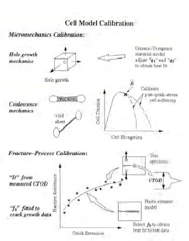
A detailed explanation of the computational cell model technique and a robust scheme for calibrating the model parameters are outlined by Faleskog (1998) and Gao (1998), and will be summarised here.
For calibrating the cell model parameters a two-step procedure as illustrated in Fig. 1 is defined. In the first step the micro-mechanics parameters, , and are estimated. The parameters and are ideally obtained by numerical computations by matching the traction vs. elongation behaviour of a GT cell with a cell containing a discrete void. If the material strain hardening is well described by a power hardening function the values given in [11] can be used. The value of the critical void volume fraction, , does not influence the resulting -curve in any significant way if it is chosen in the interval 0.10 to 0.20.
1
q q2
E
f
E
f
1
q q2
R
J
In the second step, the fracture process parameters, and D, are estimated. These are the primary parameters controlling the crack growth resistance behavior. Experimental data are required to estimate these parameters. For this purpose it is most convenient to use a -curve, but in principle any other data that accurately reflects the crack growth behavior can be used. The near tip deformation scales with the crack tip opening displacement (CTOD), which also is a relevant measure of the size of the fracture process zone. Therefore, it is reasonable to take D to be the measured CTOD at initiation of crack growth. In practice this is done by use of the relation
0
f
R
J
y IC J d D
σ
≈ (2)
where JIC is the J-value evaluated at initiation of ductile crack growth, σy the initial yield stress, and d is a non-dimensional factor ranging from 0.30 to 0.60 depending on material strain hardening and initial yield stress, Shih (1981). Once D is determined, the value of can be obtained by matching the cell model prediction to the experimentally evaluated
-curve, as illustrated in Fig. 1.
0
f
R
J
3. EXPERIMENT STUDIES 3.1 Materials
The base material employed in this investigation was an austenitic stainless steel SS2352-28. A so-called Submerged Arc Welding (SAW) process was used to weld the two 40 mm thick plates together. After welding the plate was milled down to a thickness of 28 mm. No post welding heat treatment was performed. The chemical compositions of the base and weld materials are shown in Table 1. The configuration of the welded plate is shown in Fig. 2.
Material C Si Mn P S Cr Ni Al CaF2 MgO
2352 0.014 0.4 1.16 0.033 0.002 18.1 9.1 - - -
OK Autrod 16.10 0.023 0.78 1.02 0.023 0.018 20.01 9.50 - - -
OK Flux 10.92 - 33.30 - - - 5.40 12.10 7.13 28.9
150 16 150 30o
28
40
Figure 2. Illustration of the welded plate (unit mm). The length of the plate (out plane dimension) was about 500 mm.
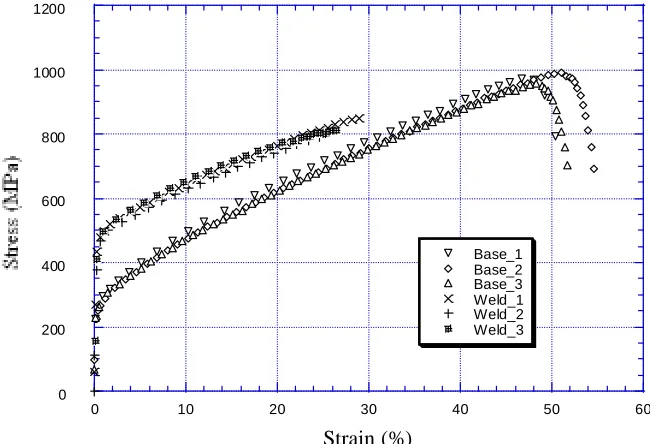
3.2 Uniaxial tensile Tests
Six standard tensile specimens were tested, three for the base material and three for the weld material. An extension-meter with a gauge length of 10mm was used to measure the tensile strain. The tests were performed at room temperature. The tensile stress-strain curves are shown in Fig. 3 for both the base and the weld materials. The offset yield strength is about 250 MPa for the base material and about 460 MPa for the weld material. The elastic modulus and Poisson's ratio are taken as 190 GPa and 0.30, respectively, which were confirmed in the uniaxial tests.
0 200 400 600 800 1000 1200
0 10 20 30 40 50 60
Base_1 Base_2 Base_3 Weld_1 Weld_2 Weld_3
Strain (%)
Figure 3. Tensile stress-strain curves for the base and the weld materials, respectively.
3.3 Fracture Mechanics Test
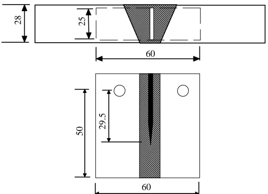
Three different configurations of plane sided (no side grooves) specimens were used in the experiments: 2 small size SE(B) specimens with square cross sections (10 mm x 10 mm), 3 standard CT specimens and 3 large size CT specimens. The cut-out position and the geometry of the specimens are shown in Figs. 4-6.
mouth to measure the so called Crack Mouth Opening Displacement (CMOD). The crack extension was estimated by use of the compliance method and the J-integral was evaluated on the basis of the force-displacement records as described in the standard.
60
10
28
48
60
10
5.
2
Figure 4. The cut-out position and the specimen geometry of the SE(B) specimen.
60
25
28
60
50 29
.5
Figure 5. The cut-out position and the specimen geometry of the standard CT specimen.
The experimental results are shown in Fig. 7. The results of the statistical mean, lower and upper bounds from the literature survey by Zang (1998) are also included in Fig. 7. It is observed that the -curves from the present experiments are within the lower and upper bounds found by Zang (1998). Furthermore it is noted that the experimental -curves from the different specimen types deviate rather little from each other. This indicates that the influence of specimen size is rather weak for the high toughness weld material.
R
J
R
120
10
10
28
120
10
0
50
Figure 6. The cut-out position and the specimen geometry of the large size CT specimen.
0 100 200 300 400 500 600 700
J-mean_literature J-low_literature J-up_literature J-SEB J-SEB J-Standard CT J-Standard CT J-Standard CT J-Large CT J-Large CT J-Large CT
-0.5 0.0 0.5 1.0 1.5 2.0 2.5 3.0
da (mm)
Figure 7. Expeimental JR-curves and results from the literature survey [3].
According to ASTM E-1737 (1997), the following size requirement should be fulfilled,
mm MPa
m kN J
b
B o y 8.3
450 / 150 25 /
25
, Ic =
⋅ ≅
≥ σ . (3)
4. COMPUTATIONAL CELL MODELLING
In this section the cell model for nonlinear fracture will be employed to analyse the experiments described in Section 3. The cell model parameters will be calibrated using the data from test on the small size SE(B) specimens. The cell model will then be used to predict the behaviour of the standard CT and large CT specimens, respectively. This scheme mimics a plausible assessment scheme based on the cell model of a flawed welded component in a nuclear power plant. The numerical computation with the finite element method was executed by use of the research code WARP3D by Koppenhoefer (1999).
4.1 Finite element model for small size SE(B) specimens
The finite element model of the small size SE(B) is shown in Fig. 8. Due to symmetry, only a quarter of the specimen is modelled. For this reason a cell element has dimensions near the free surface, whereas the thickness of a cell element inside is substantially larger than D. All elements in the mesh, including the cell elements, are eight-node trilinear hexahedral elements, and there are eight layers through the thickness. Numerical parameter studies with more than eight layers of elements were carried out, but eight layers proved to be sufficient to minimise the influence of spatial discretisation.
D D D/2)⋅( /2)⋅ (
Figure 8. Finite element mesh showing the centre plane of the small size SE(B) specimen.
4.2 Estimation of model parameters 4.2.1 Micro-mechanics parameters
In order to obtain proper values of and , the strain hardening of the material needs to be characterised. These parameters can be determined by the tensile experiments
1
shown in Fig. 7. As a results, S0 =270 MPa and n = 4.8 are obtained. According to Faleskog
(1998) the values = 1.95 and = 0.78 will best match the growth rate of a void in the current material.
1
q q2
0
P R
4.2.2 Fracture process parameters
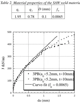
The cell size D will here be estimated according to Eq. (4). The J-value at crack growth initiation was estimated from Fig. 7 to about 100 kN/m. The yield stress, σy, and d in Eq. (2) was taken as the -value (460 MPa) and 0.46 mm, respectively. Thus, D = 0.1 mm is a suitable choice for the SAW weld material. An iterative process incorporating a sequence of finite element analyses was used to determine the initial void volume fraction in the cell elements. The best fit to the experimental -curve was obtained by = 0.0065. The
-curve from cell model is compared with the experimentally evaluated -curve in Fig. 9. The cell model parameters are summarised in Table 2.
2 .
R
J f0
R
J
R
J
Table 2. Material properties of the SAW weld material
1
q q2 D (mm) f0
1.95 0.78 0.1 0.0065
0 100 200 300 400 500
0 0.5 1 1.5 2
3PB(a
0=5.2mm, t=10mm)
3PB(a
0=5.2mm, t=10mm)
Curve-fit (f
0 = 0.0065)
da (mm)
4.3 Verification of Cell Model Technique
After the determination of all material properties, -curves for other specimen configurations and loading conditions can be predicted by the application of the cell model technique. By a comparison of the predicted and experimental -curves, the applicability of the cell model technique can be verified.
R
J
JR
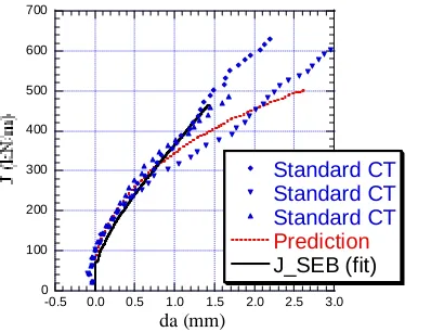
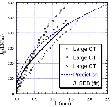
The finite element mesh for the standard CT-specimen is shown in Figure 17. A similar finite element mesh for the large size CT-specimen is used in the analysis. Nine element layers in thickness direction have been employed. The -curves showed insignificant dependence on the number of element layers if 9 or more element layers were used in the analyses. The predicted -curves and the experimental results for the standard CT-specimen and the large size CT-specimen are shown in Figs. 11-12 respectively. In these figures also the predicted -curve from the small size SE(B) specimen is included for comparison. A very good agreement between the prediction and experimental results is obtained.
R
J
R
J
R
J
Figure 10. Finite element mesh for the standard CT-specimen.
0 100 200 300 400 500 600 700
-0.5 0.0 0.5 1.0 1.5 2.0 2.5 3.0
Standard CT Standard CT Standard CT Prediction J_SEB (fit)
da (mm)
Figure 11. Experiment and model prediction of the -curves for the standard CT-specimens.
R
0 100 200 300 400 500 600
0.0 0.5 1.0 1.5 2.0 2.5
Large CT Large CT Large CT Prediction
J_SEB (fit)
da(mm)
Figure 12. Experiment and model prediction of the -curves for the large size CT-specimens.
R
J
5. FRACTURE TOUGHNESS OF IRRADIATED SMAW MATERIAL
One main purpose of the present investigation is to estimate the fracture toughness of the irradiated SMAW material if the standard CT-specimens were employed in the experiment. As demonstrated in the previous section, the cell modelling technique is capable to solve this problem if the material properties are defined.
In the following, the experimental results for irradiated small SE(B)specimens are used to estimate the material parameters. Once the calibration of the parameters is done, the cell model technique is used to predict the fracture toughness of the irradiated SMAW material.
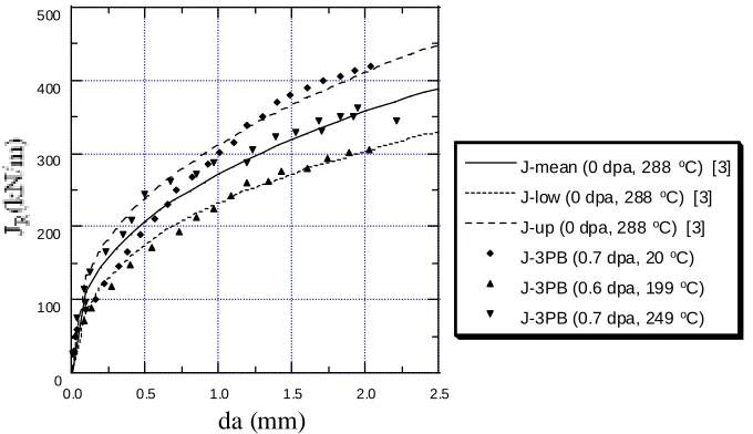
5.1 Experimental Results
Tensile and fracture mechanics tests for irradiated materials have been performed by Valo (1993). The weld is characterised as SMAW, which is another kind of weld process. The materials used by Valo (1993) were subjected to two irradiation levels (<1 dpa or <10 dpa). It was shown that ductile fracture occurs when the material is exposed to a lower neutron influence ((<1 dpa). It is therefore suitable to apply the cell model technique to material with a lower irradiation level (< 1 dpa).
0 100 200 300 400 500
0.0 0.5 1.0 1.5 2.0 2.5
J-mean (0 dpa, 288 oC) [3]
J-low (0 dpa, 288 oC) [3]
J-up (0 dpa, 288 oC) [3]
J-3PB (0.7 dpa, 20 oC)
J-3PB (0.6 dpa, 199 oC)
J-3PB (0.7 dpa, 249 oC)
da (mm)
Figure 13. Experimental results for irradiated small size SE(B) specimens.
5.2 Material Properties
The tensile tests showed that the tensile properties of the base and weld materials irradiated at about 0.7 dpa are similar to the unirradiated weld material. It can also be observed that the yielding limit both for base and weld material will only increase about 50 MPa, when the experimental temperature decreases from 270 °C to 20 °C. For convenience, the tensile properties of the unirradiated SMAW weld material tested at 288 °C will be used for the irradiated small size SE(B) specimens, even though these specimens were tested at three different temperatures. The differences from the experiments will be treated as the experimental scatter. It means that three different f0 will be obtained.
After knowing the material flow properties, the q-values can be determined by the tabulated values by Faleskog (1998). A cell size D = 0.1mm is also chosen for the material. Since side grooves have been used for the small size SE(B) specimens, a plane strain model is suitable to model these specimens. The same finite element mesh as shown in Fig. 8 was used in the numerical calculations.
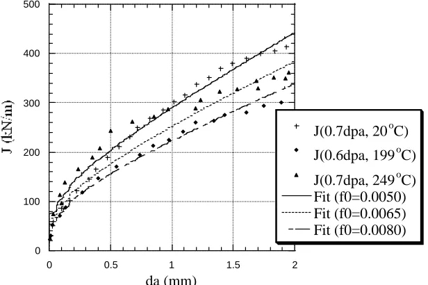
The same iterative scheme as discussed in Section 4 was used to find the best estimate of the initial void volume fraction, . The experimental -curves and the corresponding cell model predictions are plotted in Fig. 14. The micro-mechanics properties for the irradiated austenitic SMAW material are listed in Table 3.
0
f JR
Table 3. Material properties of the irradiated (< 1dpa) SMAW weld material
1
q q2 D (mm) f0
0 100 200 300 400 500
0 0.5 1 1.5 2
J(0.7dpa, 20oC) J(0.6dpa, 199oC) J(0.7dpa, 249oC) Fit (f0=0.0050) Fit (f0=0.0065) Fit (f0=0.0080)
da (mm)
Figure 14. -curves of the small size SE(B) specimens for the irradiated SMAW weld material.
R
J
5.3 Numerical Prediction
Since the initial void volume fraction was estimated based on plane strain models, a plane strain model of the standard CT-specimen will also be employed in the prediction. Thus one layer of the mesh for the CT-specimen shown in Fig. 10 was used in the calculations. Plane strain conditions were accomplished by imposing zero out of plane displacement boundary conditions on all nodes in the model.
0
f
The predicted -curves for the irradiated standard CT specimens are shown in Fig. 15. In the figure, the results for the small SE(B) specimens are also included to show the size effect on the fracture toughness of the irradiated weld (SMAW) material. It is noted that the standard size CT specimen will generate a slightly low -curve.
R
J
R
0 100 200 300 400 500
0.0 0.5 1.0 1.5 2.0 2.5
Prediction (f0=0.005) Prediction (f0=0.0065) Prediction (f0=0.008) Fit _Small_SEB (f0=0.050) Fit _Small_SEB(f0=0.065) Fit_Small_SEB (f0=0.080)
da (mm)
Figure 15 Size effect on the fracture toghness of the irradiated weld (SMAW) material.
In Figure 16, the predicted -curves for the irradiated standard CT specimens are compared to the statistical mean, lower and upper bounds from the literature study by Zang (1998) for unirradiated weld material (SMAW) tested with the standard CT specimen at 288
°C. A curve which is 20% lower than the statistical lower bound is also plotted. It can be observed that this curve covers the lower bound of the prediction. This fact implies that the effect of the irradiation at this level is very limited (only about 20%) and well within the safety margin applied in many design codes.
R
J
0 100 200 300 400 500
0.0 0.5 1.0 1.5 2.0 2.5
Prediction (f0=0.005) Prediction (f0=0.0065) Prediction (f0=0.008) J_low (0 dpa) J_mean (0 dpa) J_up (0 dpa) J_Low(0 dpa)/1.2
da (mm)
Figure 16. -curves pertaining to standard CT specimen showing the effect of the irradiation for SMAW material
R
6. CONCLUSIONS
Based on the results shown in the previous Sections, it can be concluded that:
1. The cell model technique has well captured the ductile fracture behaviour. Once the material parameters have been calibrated, the technique can predict fracture behaviour in other cracked geometry and loading configurations.
2. The specimen size has little effect on the fracture toughness for SAW weld material. Within = 2mm, -curves from the different specimens types deviate rather little from each other and within the experiment scatter. This fact has been confirmed by both experimental results and cell model simulations.
a
∆ JR
3. The specimen size has some influence on the fracture toughness for irradiated (< 1 dpa) SMAW weld material. If tested with the standard CT specimens, a lower -curve (about 20%) would be expected.
R
J
4. The fracture toughness will be decreased about 20% for the SMAW weld material after a relative low irradiation (< 1 dpa).
REFERENCES
ASTM E 1737-96, (1997)”Standard Test Method for J-integral Characterization of Fracture Toughness”. Annual Book of ASTM Standards Vol. 03.01
Matti Valo (1993),”Fracture Toughness and Tensile properties of Irradiated Austenitic Stainless Steel Components Removed from Service” Dno REA 35/91, VTT, Reactor Laboratory.
W. Zang and J. Linder (1998),”Fracture Toughness and Tensile Properties for Austenitic Stainless Steels and Welds”, SAQ/FoU-Report 98/01.
Gurson AL. (1977), Continuum theory of ductile rupture by void nucleation and growth: Part I-Yield criteria and flow rules for porous ductile media. Journal of Engineering and Material Technology; 99, 2-15.
Tvergaard V. (1990), Material failure by void growth to coalescence. Advances in applied Mechanics; 27, 83-151.
Faleskog J, Gao X, Shih CF. (1998), Cell model for nonlinear fracture analysis - I. Micromechanics calibration. International Journal of Fracture; 89, 355-373.
Gao X, Faleskog J, Shih CF. (1998) Cell model for nonlinear fracture analysis - II. Fracture process calibration and verification. International Journal of Fracture; 89, 375-398.
![Figure 7. Expeimental JR-curves and results from the literature survey [3].](https://thumb-us.123doks.com/thumbv2/123dok_us/1226742.1154473/7.595.178.418.96.315/figure-expeimental-jr-curves-results-literature-survey.webp)