CORRELATION OF STRUCTURAL MODELS FOR SSI ANALYSIS
Donald Liou1, Ai-Shen Liu2,and Yasuo Nitta3
1Senior Technologist, GE-Hitachi Nuclear Energy, USA 2Consulting Engineer, GE-Hitachi Nuclear Energy, USA 3Nuclear Division Manager, Shimizu Corporation, Japan
ABSTRACT
For licensing purposes, the Lumped Mass Stick Model for a complicated, Seismic Category I structure is correlated with the 3-D Finite Element Model of the same structure. Both models do not include the supporting soil media. The effects of using different modelling approaches are evaluated and improvements incorporated in the Lumped Mass Stick Model, which will be included in a SASSI model for the study of the Soil-Structure Interaction effects. This paper documents the correlation results, and presents some basic techniques, such as 1g Static Test and use of wall/floor oscillators, that are used to improve the Lumped Mass Stick Model. It also discusses the methods employed for modelling the underground portions of the structure in the SASSI model.
INTRODUCTION
A nuclear power plant (NPP) is conservatively designed to withstand the effects of Safe Shutdown Earthquake (SSE). As an integral part of the risk assessment, Seismic Category I and II structures in the plant may require consideration of Soil-Structure Interaction (SSI) effects in the seismic response analysis. A traditional way to capture the seismic behavior of these structures is by developing a simplified model where the building and internals are represented by mass points and beam elements, and the rock/soil/backfill underneath and surrounding the underground portions of the structure are represented by soil springs. This type of structural model is called Lumped Mass Stick Model (LMSM). On the other hand, more detailed 3-D Finite Element Model (FEM) of the same structure can be constructed for various purposes, such as stress analysis and dynamic response analysis.
In recent years, SASSI has become a common computational platform for SSI analysis of safety-related NPP structures. SASSI uses finite-element techniques and elastic half-space theory to simulate wave propagation phenomena in the soil media, and allows both LMSM and FEM representations of structure (Lysmer et al., 1981; Lysmer et al., 1999). Nevertheless, the soil portion of a SASSI model often takes a
lion’s share of the available nodal points, making FEM representation of the structure viable only for the
simplest types of structure. For SSI analysis of a complicated structure, using LMSM representation of structure is the only practical approach. Otherwise, the cost and effort associated with the SASSI analysis can quickly become prohibitive.
CUT-OFF FREQUENCY IN SASSI
SASSI is a frequency-domain program and a cut-off frequency must be specified for the SSI analysis. The cut-off frequency is selected based on frequency contents of input motion, expected SSI response characteristics, and Nyquist frequency. The selected cut-off frequency is the frequency limit at and below which the transfer functions are calculated by the program, and this frequency-limit value can be reduced from upper-bound (UB) soil profile, best-estimate (BE) soil profile, to lower-bound (LB) soil profile. For UB soil profile, the cut-off frequency can be specified at 50 Hz.
In the past, the frequency range between 25 and 50 Hz was often considered as high frequency range for seismic analysis purposes (Kassawara, 2007). USNRC acknowledged the relative inconsequence of high-frequency ground motions to equipment. In NUREG-1793 (USNRC, 2004), for example, the NRC stated
the following: “At high frequencies of vibratory excitation, the relative displacement is small and
produces insignificant increase in stress. As an example, at 25 Hz and a spectral acceleration of 1.0g, the
relative displacement is 0.016 inch. This is too small to cause damage (to critical equipment).” In recent
years, NRC position seems to have shifted. They have demanded the 50-Hz cut-off frequency for analyses of new plants located in the Eastern United States.
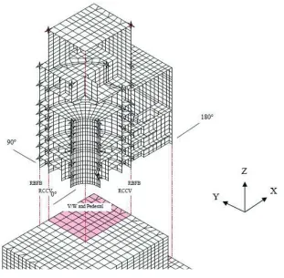
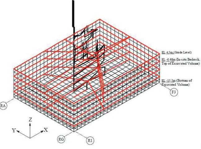
In this model correlation, the 50-Hz frequency is also used as the frequency limit at and below which the static behaviour and modal properties of the 3-D FEM and LMSM are correlated. Figure 1 shows a part of the 3-D FEM used in the correlation.
1g STATIC TEST
The correlation between the 3-D FEM and LMSM usually starts with the so-called 1g Static Test, in which static analyses are performed to both models by applying an acceleration of 1g in the X- (NS), Y- (EW), and Z- (Vertical) directions. This static test is performed before the dynamic properties, such as modal frequencies, mode shapes, and modal participation factors, are extracted from each structural model
.
To extract modal properties of a complicated 3-D FEM model often takes time; and the quality of modal properties depends upon the distributions of the mass and stiffness in each model constructed. To adjust the mass and stiffness discretization in each modelrequires both skill and patience. In comparison, 1g test is easy to perform and the output from the test is easier to interpret. The output of 1g test consists of two main categories: the internal forces in structural elements, such as support spring, and the displacements at nodal points. These output parameters are used to check major discrepancies in aggregate mass, elevation of centroid, mass discretization (e.g. distribution to the mass points), and stiffness discretization in the models. The output from 1g test is also used for estimating the mode shape and modal frequency of the fundamental mode of the structure in each direction.Table 1: Summary of 1g Test Results
LMSM
FEM
X
–
Dir. Total
Base Shear (MN)
1,870
1,871
Y
–
Dir. Total
Base Shear (MN)
1,871
1,871
X
–
Dir. Total
Base
Moment (MN-m)
44,653
44,785
Y
–
Dir. Total
Base
Moment (MN-m)
47,783
45,917
Total
Axial Force (MN)
1,869
1,871
X
–
Dir. Top
Deflection (mm)
18.3
17.1
Y
–
Dir. Top
Deflection (mm)
22.6
19.2
Z
–
Dir. Top
Deflection (mm)
3.07
2.64
X
–
Dir. First Mode
Frequency (Hz)
3.7
3.8
Y
–
Dir. First Mode
Frequency (Hz)
3.1
3.6
Z
–
Dir. First Mode
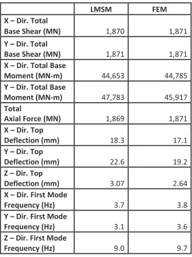
Table 1 summarizes the key results of 1g test of the structure models studied. In this table the selected output from the 1g tests of both 3-D FEM and LMSM are listed side by side for easy comparison. For each horizontal direction, the selected output includes the total base shear, the total base moment, and deflection at the top of structure. For vertical direction, the selected output includes the total axial force at base, and the nodal deflection at the top of structure.
A check of the total mass in each model is performed by comparing the reaction forces at the base of the structural model (e.g. the total axial force or base shear). As indicated by the table, the base forces from the models are reasonably close. For each horizontal direction, the ratio between the total base moment
and the total base shear indicates the location of the structure’s centroid in that direction. Although not as
close as the comparison of aggregate masses, the locations of the structure’s centroid in each horizontal
direction of the models are also reasonably close.
Although not shown in Table 1, the displaced shapes of the structure under the 1g test are generally listed in the same table for easy comparison. A displaced shape can be represented by the deformations at selected nodes plotted along the height of the building. The displaced shapes of the structure predicted by FEM and LMSM under the 1g analysis must be relatively close in order to assure that the stiffness representations and mass distributions in the models are consistent. In addition, for Safety-Related structures that are, predominantly, concrete shear-wall structures, their horizontal deformed shapes may be characterized by a gradual increase in total displacement as the elevation increases (Ratnagaran et al., 2014).
Of the displacements at the selected nodes, the displacement at the top of the structure, ∆, is the most
important; and they are the only deformation values listed in Table 1. This deflection value can be used for estimating the fundamental-mode frequency of a structure in each direction (Thomson and Dahlen, 1998). The estimated fundamental-mode frequencies for the structure studied are also given in the bottom rows of Table 1.
INCLUSION OF WALL/FLOOR OSCILLATORS IN LMSM
Each floor slab, structural wall, or other local structural component that has a modal frequency of vibration below the cut-off frequency can be directly represented in the LMSM by using a wall/floor oscillator. Such vibration mode is called flexible mode. A floor oscillator, with proper values of mass and stiffness, is added to the base model so that the vertical In-Structure Response Spectra (ISRS) and the maximum vertical acceleration response at the location of the oscillator can be generated for the flexible portion of a floor slab. Similarly, a wall oscillator can be added to the base model for the generation of horizontal ISRS and the horizontal acceleration response at the flexible portion of a wall. This involves eigenvalue extraction, identification of flexible modes and their locations in the LMSM model, and specification of oscillator parameters.
The FEM, primarily built for stress analysis purposes, is used to extract the modal properties of floor slab, structural wall, and other local structural components by assigning proper boundary conditions in the model. For example, in order to extract the modal properties of a particular floor slab in the FEM, portions of supporting walls are included in the floor slab model so the flexibility of the slab/wall joint is properly accounted for in the eigenvalue analysis for that floor slab alone.
Figure 2. Eigenvalue Analysis Result for a Slab in the 3-D FEM Model
A floor oscillator with a frequency of vibration of 23.64 Hz is added to the LMSM to represent the vertical vibration of the first-quadrant portion of this floor. The mass and stiffness values of the floor oscillator in the LMSM is so tuned that the frequency of vibration of the oscillator matches the mode of vibration of the floor that the oscillator represents, as shown in Figure 2. As the oscillator mass value will be less than 100% of the total mass of the floor in the FEM, the balance of mass should be distributed to other appropriate mass points in the LMSM.
INSERTING OUTRIGGERS FOR ISRS GENERATION
Major equipment must be qualified by using the relevant, representative ISRS with appropriate damping ratios. However, this is often not an easy task. Firstly, the SSI analysis is often performed in the licensing phase of a project. In this phase, the locations of major equipment are not all finalized. The conservative approach is to generate ISRS at building edges where the coupling effects between vertical and rocking and between lateral and torsion motions are most pronounced. The most common way is by inserting outrigger rigid-beam elements at appropriate levels of the LMSM model so the responses at the building edges can be computed directly.
MODAL PROPERTIES COMPARISON
In each structural model, modes extracted are the orthogonal coordinates of the linear, elastic representation of the structure studied; and modal properties produced by eigenvalue analysis include frequencies of vibration, mode shapes, and participation factors. For a complicated structure, the direct comparison of the eigenvalue analysis results is not always straightforward. An important mode in the LMSM analysis, with less DOF, can be identified by the associated large participation factor. The same mode in the FEM analysis, with much more number of DOF than that in LMSM, may or may not split. If a dominant mode is split, the participation factor will also split, resulting in many modes with little variation in frequency of vibration. Thus, the modal comparison should be performed between a dominant mode produced by the LMSM analysis and all modes in a certain range of frequency produced by the FEM analysis.
If the modal properties correlation between the LMSM and FEM analysis for the dominant modes is poor, there are at least two possibilities. If it is believed that the FEM analysis produces better results, tuning of the LMSM may be necessary. Here, tuning of the LMSM model is used to mean changing the stiffness matrix and re-distribute the mass matrix of the model so that the corresponding modal properties will better correlate with those of FEM analysis. If it is the other way around, the FEM may have incorrect input and must be checked more thoroughly. Either way, the modal properties correlation will impact the SSE response comparison, which is discussed in the next section.
SSE RESPONSES COMPARISON
Assuming the structure has fixed, surface-foundation, seismic time history analyses can be performed using the FEM and LMSM models and the results can be compared equitably. The fixed base assumption excludes all effects that can be caused by embedment and SSI. In order to produce maximum seismic responses for comparison, simultaneous X-, Y- and Z- direction SSE ground-motion input and modal damping ratio of 7.0% for each mode are used for both analysis models. The SSE analyses produce responses, such as maximum response accelerations at each floor level, which can be used in the cross-evaluation of the models.
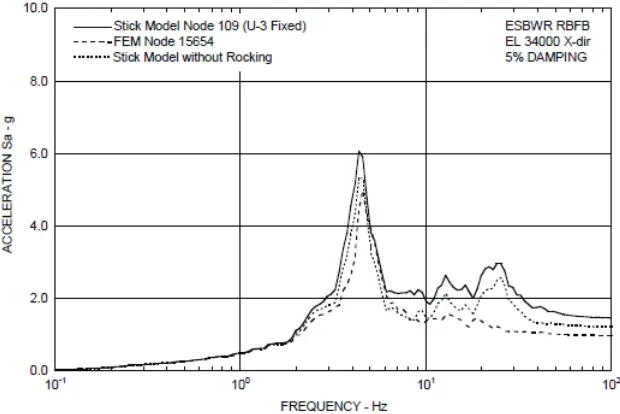
Figure 3. Horizontal Response Spectra Comparison at A High Elevation
curves and two of the curves are produced by two different LMSM models. One of the LMSM model considers the coupling effects between vertical and rocking and between lateral and torsion, and the other does not. As shown in this figure, the peak frequency, magnitude, and general shape of these ISRS curves compare well in the low frequency range, even before these curves are broadened for equipment qualification purposes. After broadening, any differences between the ISRS curves produced by the models would become insignificant in the low frequency range. In the high frequency range the ISRS curve from the LMSM model with coupling effects is higher than the FEM ISRS.
MODELLING UNDERGROUND PORTIONS OF STRUCTURE
The computer program SASSI utilizes the substructure approach in which the linear SSI problem is divided into sub-problems based on the principle of superposition using linear material properties. The soil portion, including original rock and soil materials, structural backfill, and concrete fill, can be modelled using 3-D brick (solid) elements. If LMSM is used for the structure, modeling of the underground portions of the structure need to be compatible with that of the soil portion. There are different ways to achieve this. One of them is to model only the embedded, outside faces of the structure and tie these faces to the appropriate nodal points in the structure stick.
Figure 4 illustrates how the embedded outside walls of the structure can be modelled by using shell/plate elements. In this figure, these walls are stiffened at the floor levels and tied to the structure stick by using rigid beams. These rigid beams are colored in red. As the shell/plate elements that are used to represent the embedded, outside walls have mass and stiffness of their own, the below ground portions of the LMSM must be adjusted accordingly.
Figure 4. Modelling Underground Portions of Outside Wall for SASSI
Using SASSI terminology, the underground portions of the structure which are enclosed by the outside
walls on the sides and the basemat from below is called “excavated volume.” Excavated volume and
physical location, i.e. the same X-, Y-, and Z-coordinates. Such nodes are called “double nodes.” SASSI
allows spring constants to be inserted to the global stiffness directly at these double nodes so that the forces across the interface during the seismic excitation can be approximated. Along with restrictions on the mesh size and aspect ratio of element, each version of SASSI places an upper limit to the total number of interaction nodes. SASSI2010, for example, limits to interaction nodes to no more than 20,000.
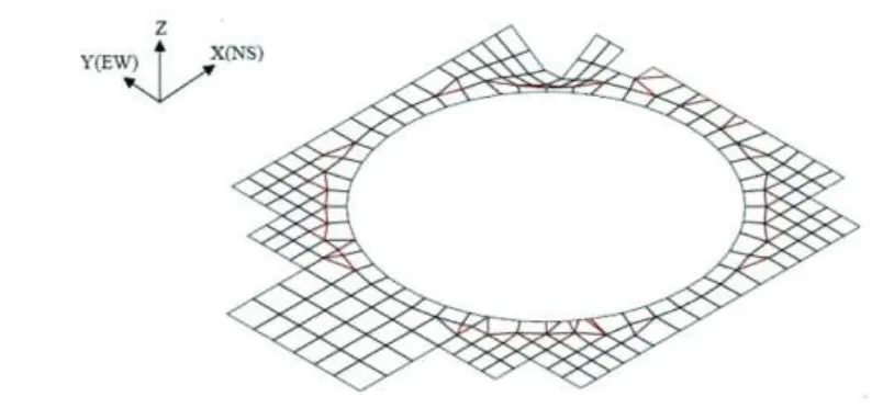
Besides the embedded portions of the outside walls, the embedded faces of the excavated volume include the base-mat. The base-mat is strengthened by the inner shear walls, as shown in Figure 5. It can be modelled in the same way as the outside walls, i.e. with shell/plate elements that are stiffened by rigid beams and with double nodes at the interface with supporting medium.
Figure 5. Shear Wall above the Basemat
CONCLUSIONS
The Lumped Mass Stick Model and the 3-D Finite Element Model for a complicated, Seismic Category I structure are correlated. The correlation results are used to improve the stick model, which is embellished with inclusion of wall/floor oscillators and insertion of outriggers at the appropriate nodes. The calculated ISRS curves generated by the two models compare well in terms of peak frequency, magnitude, and general shape while the LMSM curve with coupling effects tends to be higher. After broadening, any differences between the ISRS curves would become insignificant, making the stick model the structural representation of choice in the SASSI Soil-Structure Interaction analysis. The methods employed for modelling the underground portions of the structure in the SASSI model are also discussed.
REFERENCES
Lysmer, J., M. Tabatabaie-Raissi, F. Tajirian, S. Vahdani, and Ostadan F., “SASSI-A System for Analysis of Soil-Structure Interaction,” Report no. UCB/GT/81-02, Department of Civil Engineering, University of California, Berkeley, 1981.
Kassawara, R., “Seismic Screening of Components Sensitive to High Frequency Vibratory Motions,”
EPRI white paper, 2007, ML072600202.
U.S. Nuclear Regulatory Commission, “Final Safety Evaluation Report Related to Certification of the
AP1000 Standard Design,” Report NUREG-1793, September 2004.
Thomson, W. T., and Dahlen, M. D., “Theory of Vibration with Applications,” 5th Ed., Prentice Hall,
1998.
Ratnagaran B., Torkian1 B., Chandran P., and Lu S., “Soil Structure Interaction Analysis of a Boiling
Water Reactor Building,” Proceedings of ICAPP 2014, Charlotte, USA, April 6-9, 2014.