A Prototype Hadamard Imaging System

ABSTRACT

Fothergill, Daryl William. A Prototype Hadamard imaging system (Under the direction of Dr. John Muth.)

The purpose of this thesis was to investigate the possibility of creating an inexpensive

imaging system that would be suitable for imaging small animals, either the skin of mice for

skin cancer studies, or potentially whole animal imaging. In this optical system the light is

collected by an array of 31 optical fibers. In more advanced systems one can envision 1024,

or even more fibers being used to increase the resolution of the image. The principle novelty

of this system is that Hadamard encoding enabled only one photodetector to be used for the

whole system rather than one detector for each fiber. There are two important advantages

that can be obtained by using this strategy. First, especially with large numbers of fibers, the

overall signal to noise ratio of the system can be improved. Second, the cost and complexity

of the system can be greatly reduced. In cases where the signal to noise ratio is low, such as

fluorescence detection, designing a system that has only one detector has substantial

advantages. This system can also be applied to other sensor applications with large numbers

of inputs. To our knowledge Hadamard imaging has not been applied to macroscopic

imaging applications, or to small animal imagining.

Plastic fiber optics are used to gather and pixilate the spatially dependent inputs from

the light source. The optical fibers were then switched on and off using a rotating mask

encoded with a Hadamard matrix by drilling holes in the mask. The encoded light was then

detected with an inexpensive photodetector and decoded using a desktop computer. The

system is automated by using a BASIC Stamp to control the stepper motors and LabVIEW.

Future improvements such as a stationary MEMS mask and glass optical fibers that could

A PROTOTYPE HADAMARD IMAGING SYSTEM

by

DARYL WILLIAM FOTHERGILL

A thesis submitted to the Graduate Faculty of

North Carolina State University

in partial fulfillment of the

requirements for the Degree of

Master of Science

ELECTRICAL ENGINEERING

Raleigh

2005

APPROVED BY:

____Dr. Robert M Kolbas___ ___Dr. David S. Lalush_

_____Dr. John F Muth___________

BIOGRAPHY

After graduating high school in 1999, I spent two years at Lehigh University in

Bethlehem, PA studying Electrical Engineering. I transferred to North Carolina State in

2001 and graduated Magna Cum Laude in December 2003 with B.S. Electrical Engineering

and B.S. Computer Engineering degrees. During most of my time at NCSU, I have been

working with Dr. Muth in some manner. This thesis will conclude my M.S. Electrical

Engineering degree. My career as an engineer will begin with Northrop Grumman-Electrical

TABLE OF CONTENTS

PAGE

LIST OF TABLES... v

LIST OF FIGURES... vi

1. INTRODUCTION... 1

1.1 Principle novelty... 1

1.2 Motivation... 2

2. IMAGING AND COMPONTENTS OVERVIEW... 4

2.1 Imaging overview... 4

2.2 Fabricated Hadamard imaging system... 6

2.3 Methods of imaging... 8

2.3.1 OCT using light induced fluorescence... 8

2.3.2 Optical fiber sensors... 9

2.3.3 Smart skin... 12

2.4 Optical imaging components... 12

2.4.1 Photodetector... 13

2.4.2 Fiber optics... 17

2.4.3 Mask... 18

3. THE EFFECT OF MULTIPLEXING ON SPATIAL ENCODING... 20

3.1 Spatial encoding... 20

3.2 Multiplexing... 22

4. INTRODUCTION OF HADAMARD SPECTROPSCOPY... 25

4.1 Spectroscopy... 25

4.2 Hadamard spectroscopy... 28

5. HADAMARD IMAGE RECONSTRUCTION... 31

5.1 Basic Hadamard mathematics... 31

5.1.1 Weighing scheme... 31

5.1.2 Matrix mathematics... 36

5.2 Simple correction matrix... 39

6. EXPERIMENTAL APPARATUS... 41

6.1 Hardware... 41

6.1.1 Motors... 42

6.1.2 Optical fibers... 42

6.1.3 Hadamard pattern, number of elements... 44

6.1.4 Mask and fiber mounts... 44

6.1.5 Lenses... 48

6.1.6 Photodetector... 49

6.1.7 Custom light source tube... 50

6.1.8 Light source and black box... 51

6.2 Software... 51

PAGE

6.2.2 LabVIEW, PCI Board, Matlab... 53

7. PROOF OF THEORY... 54

7.1 Overview... 54

7.2 Data collection and fiber placement... 54

7.3 Fiber alignment with mask... 56

7.4 Single fiber testing... 57

7.5 Repeatability... 62

7.6 Multiple fiber testing... 62

7.7 2-D imaging of 3-D object... 66

7.8 Problems with this system... 69

8. FUTURE IMPROVEMENTS... 72

8.1 Overview... 72

8.2 Stationary programmable mask... 72

8.2.1 MEMS mask... 72

8.2.2 Electrooptical mask... 77

8.3 Glass optical fibers... 79

8.4 KOH etch v-grooves in bulk silicon... 80

8.5 Future work conclusions... 84

LIST OF REFERENCES... 85

APPENDIX... 88

A.1 Parts list... 89

A.2 Plastic fiber optic spec sheet... 90

A.3 Hadamard matrix used... 91

LIST OF TABLES

PAGE Table 7-1 Single fiber source and output data ... 59

Table 7-2 Linearity of photodetector without bias... 64

LIST OF FIGURES

PAGE

Figure 2-1 Basic optical imaging... 4

Figure 2-2 Human eye verses CCD camera... 6

Figure 2-3 Schematic representation of thesis imaging system.... 7

Figure 2-4 Model of endoscope tip... 9

Figure 2-5 Master plan for OFPT... 11

Figure 2-6 Schematic representation of APD... 15

Figure 2-7 Spectral analysis of absorption coefficient... 17

Figure 3-1 Nipkow disk... 21

Figure 3-2 SNR advantage (Q) dependence on N... 24

Figure 4-1 Michelson interferometer... 26

Figure 4-2 Normalized intensity as a function of time... 27

Figure 4-3 Prism dispersing light... 28

Figure 4-4 Optical schematic of 255-slots HTS... 29

Figure 5-1 Examples of Hadamard matrices... 35

Figure 5-2 Examples of S-matrices... 35

Figure 5-3 Basic block diagram of a multiplexing system... 37

Figure 5-4 Matrix representation of Hadamard imaging... 37

Figure 6-1 Hadamard imaging system constructed... 41

Figure 6-2 Plastic fiber characteristics... 43

Figure 6-3 32 ‘on’ bits in pie shape... 45

Figure 6-4 Hadamard mask in Eagle Soft... 46

Figure 6-5 31 single hole array... 46

Figure 6-6 Photodetector fiber mount... 47

Figure 6-7 Mask and mounts designs... 48

Figure 6-8 Large area UDT photodetector... 49

PAGE

Figure 6-10 Light sources... 51

Figure 6-11 BASIC Stamp and motor drivers... 53

Figure 7-1 Mask and fiber mount clamped from side... 57

Figure 7-2 Hadamard representation of fiber 5 illuminated... 60

Figure 7-3 Relative intensities with microscope lamp... 60

Figure 7-4 Relative intensities with fluorescent lamp... 61

Figure 7-5 Repeatability graph... 62

Figure 7-6 Multiple positions illuminated no bias, 7 and 25... 63

Figure 7-7 Multiple positions illuminated no bias, 15-17... 63

Figure 7-8 7 & 25 positions illuminated w/ bias, (ideal)... 65

Figure 7-9 15-17 positions illuminated w/ bias, (ideal)... 65

Figure 7-10 Multiple positions illuminated w/ bias, 15-17... 66

Figure 7-11 Example test tube spiral pattern... 67

Figure 7-12 2-dimensional spiral pattern... 68

Figure 7-13 3D representation of spiral scan... 68

Figure 7-14 3D normalized representation of spiral scan... 69

Figure 7-15 Misalignment example of light at fiber 30... 70

Figure 8-1 Deformable mirror device... 73

Figure 8-2 Basic deflection principle... 74

Figure 8-3 Electrical schematic of DMD mirror... 75

Figure 8-4 Schematic of a mirror with bending arms... 76

Figure 8-5 Steps of the micromirror production... 77

Figure 8-6 Vanadium dioxide optical properties... 78

Figure 8-7 3-D view of square feature etched into Si substrate.. 81

Figure 8-8 Silicon etch rates in KOH... 81

Figure 8-9 Process development for KOH etch... 83

CHAPTER 1

INTRODUCTION

1.1 Principal novelty

The purpose of this thesis was to investigate the possibility of creating an inexpensive

imaging system that would be suitable for imaging small animals, either the skin of mice for

skin cancer studies, or potentially whole animal imaging. In this optical system the light is

collected by an array of 31 optical fibers. In more advanced systems one can envision 1024,

or even more fibers being used to increase the resolution of the image. The principle novelty

of this system is that Hadamard encoding enabled only one photodetector to be used for the

whole system rather than one detector for each fiber. There are two important advantages

that can be obtained by using this strategy. First, especially with large numbers of fibers, the

overall signal to noise ratio of the system can be improved. Second, the cost and complexity

of the system can be greatly reduced. In cases where the signal to noise ratio is low, such as

fluorescence detection, designing a system that has only one detector will be a substantial

advancement.

To perform the imaging in this thesis, the Hadamard encoding was accomplished by

using a rotating mechanical mask with holes. Depending on the position of the mask the

light was selectively admitted or blocked. In the case of this prototype system, there were 31

fibers used. Therefore a mask with 31 Hadamard patterned positions was used, plus two

extra patterns for a complete on and complete off. The extra two patterns were used to

one open hole per each mask position, the image could still be reconstructed. However in

our case, each of 31 positions had 16 open holes and 15 closed holes. The advantage of this

is that at any one time about of the total light of the image is incident on the detector.

Thus the detector always has a strong and roughly constant signal to noise ratio for any of the

31 positions of the mask. In the body of the thesis we will show that if the mask

combinations are determined using a Hadamard Matrix, the inverse of the matrix can then be

used to recover the image. To our knowledge Hadamard imaging has not been applied to

macroscopic imaging applications, or to small animal imagining.

1.2 Motivation

As a motivation for a potential application of this work we will consider the detection

of skin tumors in hairless mice, and other small animal imaging applications. It has been

shown since 1908 that tumor tissue autofluoresces differently than the surrounding

non-cancerous tissue.1 In the field of biophotonics, laser and chemical induced fluorescence has

been used to identify tumors, but have not yet progressed into clinical studies.1,2,3 In these

studies, imaging is typically not performed, just the comparisons of differing amounts of

autofluorescence from tissue samples. In the case where imaging is performed, a good signal

to noise ratio is a problem because of the detection methods and detectors being used. Thus

it would be advantageous to be able to spatially resolve the autofluorescence of small tumors

from the surrounding tissue. Presently researchers use genetically engineered mice to study

skin cancers. These special mice are very susceptible to skin cancer, and after being dosed

with UV light will develop tumors within a very well defined time period. However,

microscope. There is also a minimum size tumor of about millimeter that can be detected by a skilled researcher feeling the skin of the mouse. It would be beneficial to have a way to

detect tumors earlier, and nondestructively. It would also be helpful to monitor the effects of

tumor killing drugs on the size of the tumor over time, rather than killing the mouse at

different numbers of days after exposure to the UV radiation. With respect to human

inspection of skin cancer, a visual inspection is performed with a magnifying glass allowing

for especially small tumors to go unnoticed. If tumor precursors could be identified by

optical imaging with a handheld instrument, it would be a significant advantage. The fact

that tumor tissue emits a different kind of light than the surrounding tissue suggests a means

by which the tumor can be detected optically.

The other potential application of this tool is to reconstruct 3 Dimensional images of

small animals. Since the optical fibers can be placed anywhere with respect to the animal,

one can envision surrounding the animal with optical fibers. Shining the light into the animal

and collecting the light that makes it through the animal, or in other cases collecting

fluorescence from the animal one could reconstruct a 3-dimensional image of the animal.

This system can also be applied to sensor applications with large numbers of inputs and fiber

optic sensors

This thesis demonstrates a working model of a Hadamard imaging system. Basic

imaging characteristics were studied and simple test pattern images were obtained. The

mathematics of the Hadamard and Inverse Hadamard transform were investigated along with

CHAPTER 2

IMAGING AND COMPONENTS OVERVIEW

2.1 Imaging overview

It is useful to consider a simple imaging system as being composed of three parts, the

object, the lens, and the screen where the image is detected as shown below in Figure 2-1.

Figure 2-1: A simple demonstration of imaging with single lens [4]

The surface of an object is either self-luminous or externally illuminated as if it consisted of a

very large number of radiating point sources. Each of these point sources emits spherical

waves; rays which radially emanate in the direction of the energy. The lens redirects the

wavefronts and depending on the position of the screen with respect to the focal point an

upright or inverted image will be obtained. If the screen is at the focal point the Fourier

transform of the image is obtained.

The most impressive and most commonly used example of an imaging system is the

lens arrangement that casts a real image on a light sensitive retinal surface made up of about

120 million rods and 7 million cones. This notion was proposed by Kepler (1604), who

wrote “Vision, I say, occurs when the image of the … external world … is projected onto the

... concave retina.”5

As the light first enters the eye, the cornea serves as the first and strongest convex

lens system. Light emerging from the cornea passes through a chamber filled with a clear

watery fluid called the aqueous humor. Immersed in this is a diaphragm known as the iris

which serves as the aperture to control the amount of light entering through another hole, the

pupil. The light is then focused by a crystalline lens through the vitreous humor onto the

back of the eye ball on a thin layer of light receptor cells called the retina. The focused beam

of light is absorbed via electrochemical reaction in this multilayered structure. There are two

kinds of photoreceptor cells: rods and cones. Roughly 125 million of them are intermingled

nonuniformly over most of the retina, each acting as its own pixel. The ensemble of rods

(.002mm in diameter) in some respects has the characteristics of a highspeed, black and

white film. It is exceedingly sensitive performing in light too dim for the cones to respond

to, yet it is unable to distinguish color, and the images it relays are not well defined. In

contrast, the ensemble of 6 to 7 million cones (.06mm in diameter) can be imagined as a

Figure 2-2: Human eye verses CCD camera [5]

The idea that an image can be interpreted as an array of individual detector elements

is an important one. In film the individual silver grains act as detectors and determine the

resolution. In digital cameras the size of the pixel elements determines the resolution. With

detector arrays, as represented by a CCD camera (Figure 2-2), we can consider the image to

be defined as an array of individual pixels. This lets one break the image up into discrete bits

of information which can be manipulated electronically. The use of smaller sized pixels and

larger numbers of pixels generally imply higher spatial resolution. Ultimately the resolution

is limited by the aberration and diffraction limits of the optics used to form the image.5

2.2 Fabricated Hadamard imaging device

A schematic representation of the system is shown in Figure 2-3. This system is

capable of spatial dependent surface light detection. The system patterns the light from the

light source via a rotating mask. For each position of the mask the data is collected using a

single photodetector and the inverse of the Hadamard matrix is used to obtain the image.

This is possible because the fibers are spatially numbered and in turn the spatial position is

Figure 2-3: Schematic representation of thesis imaging system

The imaging system presented in this thesis is directed towards being used for surface

optical imaging such as in the case of small animals for the detection of skin cancer. For this

to be possible the tumor (skin cancer) will need to be “activated” in such a manner where it

will emit fluorescent light. It is important to briefly look at the two methods of doing this.

One method is an injection which will provide for a chemical reaction throughout the small

animal allowing for immediate detection over the entire glowing source. This method is

known as bioluminescence. The second is noninvasive laser induced fluorescence (LIF),

which is a new and currently evolving technology. Multiple researchers have demonstrated

the use of LIF to differentiate normal tissue form cancer and pre-cancer tissue. Excitation

wavelengths at 330, 370, and 430nm were found to be the most useful for discriminating

normal from malignant tissue.6 The first source of autofluorescence is the simpler case, but

the later is preferred because it is noninvasive and more applicable to human usage.

LIF requires alignment management between the laser that is doing the fluorescing

and the optics that is collecting the fluorescent light. The amount of fluorescent light that is

emitted from a tumor is proportional to the intensity from the laser on the tumor. As the

the laser at the same section of skin to have a proper scan. This was not brought into the

fabrication of the optical imaging system presented in this thesis, but this system could be

modified to perform this type of surface imaging.

2.3 Methods of imaging

There are plenty of methods of imaging using optical fibers. The following are a

layout of some of these methods.

2.3.1 OCT using light induced fluorescence

Optical coherence tomography (OCT) is a non-invasive imaging technology offering

up to multiple millimeter penetration with multiple sub micrometer axial and lateral

resolution. Images are produced by low-coherence interferometry in which coherence

patterns are used to reproduce image. This uses the basic principles as Michelson

interferometry which will be fully discussed in Chapter 4. Such a device combined with LIF

as previously described in this chapter has been used to provide for micron resolution over a

surface of 6mm for optical imaging of cancerous tissue.6 The components and reconstruction

system used within this system will show to be far more complex than the Hadamard

imaging system. The technical challenge in combining OCT and LIF is to meet the

drastically different requirements of each system in the same minute package. OCT requires

a focused near-IR beam for deep (~2mm) tissue penetration. LIF usually excites the tissue

with a monochromatic beam of relatively short (UV-green) wavelengths light with shallow

tissue penetration (~200µm from 325nm). The design of a LIF system must be optimized at

concern. Special optical fibers were designed so that the OCT and LIF excitation beams

were nearly coaligned on the sample as shown in Figure 2-4. One can see the complexity of

this component. Spectral readings were coregistered with OCT readings, accounting for the

offset between the beams in the tip optics and the scan difference covered during the spectra

acquisition. Different wavelengths for LIF were used to accomplish a slight sense of depth

measurements. All of this provides for a more complex system than the Hadamard imaging

system presented which simply has to count photons instead of looking at interference

patterns. This does show that LIF can be used for imaging of skin cancer and that a simpler

system is needed to do so.6

Figure 2-4: a) shows the focused IR for OCT (O) as well as the diffuse UV illumination (E), b) model of endoscope tip [6]

2.3.2 Optical fiber sensors

Optical fiber process tomography (OFPT) based on optical fiber sensors (OFSs), has

process monitoring and control. Sensors that use such a system instead of x-ray or electrical

capacity have the following advantages:

1. It is suitable for low-density medium because optical intensity is sensitive to

medium attenuation.

2. It can be used to small and irregular spaces owing to the small volumes of OFS

probes.

3. It is safe and free of electromagnetic interference since the medium’s information

is transformed into optical signals and processed remotely.

4. It can make a distributed OFPT measurement system possible using the high

speed and wide bandwidths of OFS.

Different forms of OFPT can measure the media distributions and contents in the

interrogated area, such as the measurements for two-phase flows. The system operates based

on the optical transmission characteristics in the medium.7 For the case of parallel rays and

uniform medium, the optical intensity of a luminous beam is found by the Lambert formula

) exp( L I

Iout = in (2-1)

where Iin and Iout are the optical intensities of input and output rays respectively, is the

optical attenuation coefficient, and L is the optical length in the medium. Knowing Iin and L

and detecting Iout, one can solve for . Due to the pixilation and optical scheme as shown in

Figure 2-5, the optical intensities detected and processed by photodetectors the medium

distributions could be worked out by solving the equation based on Eq. (2-1).

The aspect involved in the design of OFPT which relates to structures is the pixel distribution

to divide the measured region into pixels for image reconstruction and media information

into a pattern of pixels that sustains the circular symmetry (shown in Figure 2-5) in which

flow and fluid level can be accurately sensed directly within the cylindrical contain. It is

important to point out that each fiber has its own detector after the light has traveled through

the medium.

Figure 2-5: Master plan for OFPT [8]

Several algorithms are mentioned as possible uses for this tomography image

reconstruction, such as linear back projection, filtered back projection, algebraic iterative

reconstruction, Radon transformation, and Fourier transformation algorithm.8 Collecting

sufficient data is difficult due to the fact that optical transmission in the media interface is

very complex because many optical phenomena may be happening such as scattering, diffuse

reflection, and refraction. A parallel light ray may be changed into a partly diverging light

ray in the interface. This leads one to believe that the less noise created by the reconstruction

scheme would be greatly desired. Using a Hadamard scheme to gather the light to a single

detector while patterning the light would be a simple solution to this project. The optical

signals are already being coupled back into optical fibers after traveling through the media.

Couple all of these signals to a single photodetector patterned by a stationary mask made up

ratio. The information will also stay in pixilated form as Hadamard math is done with matrix

multiplication.

2.3.3 Smart skin

Hadamard imaging has been researched for optical fiber smart skin sensing

applications which include stress monitoring, fatigue detection, and temperature sensing.9

This idea of monitoring the status of composite materials via embedding an optical fiber

within or on top of the material is done such that real time monitoring of the material status

can be performed. Some military applications are the status monitoring required to

determine the long term reliability of conical-shaped composite bobbin structures that

support multiple layers of fiber optic cable under tension. A conventional approach uses a

single fiber which can only provide monitoring of one-dimension. To obtain broad profile

monitoring across the surface of the composite, an array of fibers is proposed using a

Hadamard transform so only a single photodetector is necessary. This will allow for a cheap

and compact two-dimensional system.

2.4 Optical imaging components

In our system the most important optical imaging components are:

1. The photodetector for the measurement of light intensity.

2. Fiber optics to pixilate the optical source and light transportation.

The purpose of this project was to perform a proof of concept demonstration, so the principal

criteria used to evaluate components were cost and ease of use. In the following sections

some of the design choices are considered.

2.4.1 Photodetector

The perfect photodetector would detect all incident photons of the desired

wavelength, and would have a fast response. However, our choice of detectors consisted of

photodiodes, photomultiplier tubes (PMT), avalanche photodiode (APD), and charge coupled

devices (CCD).10

• Photodiode – A Photodiode in its simplest form is a p-n heterojunction in which a P+

layer is put in an N substrate (or other way around) by diffusion or ion implantation.

Charge balance causes electrons from the N side to rush into the P+ layer while holes

from the P+ rush into the N layer. This neutralization and charge separation results in

an electric field at the junction that separates the photogenerated electrons and holes

resulting in a photocurrent. Electrons and holes generated away from the depletion

layer are not affected by electric field and most likely are lost in surface

recombination. These recombined carriers do not contribute to a signal to the

external circuit.

• PMT – Such photodetectors are based on photoelectric emission which usually

operates in a vacuum tube called phototubes. When light comes into contact with the

photoemissive material (cathode), electrons are emitted and travel to an electrode

transport between the cathode and anode, an electrical current proportional to the

photon flux created in the circuit. The photoemitted electron may also impact

another specially placed metal or semiconductor surfaces in the tube, called dynodes,

from which a cascade of electrons are emitted by the process of secondary emission.

The result is an amplification of the generated electric current by a factor as high as

107.

• APD - A more complex photodiode design known as an avalanche photodiode which

operates by converting each detected photon into a cascade of moving carrier pairs.

Weak light can then produce current that is sufficient to be readily detected. A

schematic representation is shown in Figure 2-6. A photon is absorbed at point 1,

creating an electron-hole pair. Under the effect of the strong electric field the

electron is accelerated increasing its energy with respect to the bottom of the

conduction band. This process is constantly interrupted by random collisions with

the lattice in which the electron loses some of its acquired energy. At point 2, the

electron has acquired enough energy ( > Eg) generated a second electron-hole pair by

impact ionization. The two electrons then accelerate under the electric field and

further impact ionization to continue to create more electron-hole pairs. Gain is

achieved, but APDs suffer from an additional multiplication time in responsivity.

• CCD - The CCD imaging system is a circuit of small semiconductor devices forming

an array of pixels on which the image is focused. The core of the CCD imaging

semiconductor (MOS) capacitor. The incident photons release a charge in the

semiconductor device that can be stored as well as shifted around the array and

eventually detected by a sequence of clock signals applied to the devices. In

depletion mode, the MOS device can be modeled similar to an abrupt p-n junction

under reverse bias that will allow charge to accumulate when exposed to incident

light. Each MOS capacitor acts as its own detection device creating individual small

active areas or pixels allowing for the high precision and resolution.

Figure 2-6: Schematic representation of APD [10]

Noise in a photodetector is undesirable but does exist and will result in small amounts

of current flow even when no light is incident on the detector. This is known as “Dark

Current”. Additional noise in a photodetector comes in the form of Shot Noise, Flicker

Noise, and Thermal Noise.

• Shot noise consists of random fluctuations of the electrical current which are

caused by the fact that current is carried by discrete charges (electrons). The

strength of the noise will increase with the magnitude of average current flowing

through the photodetector. Thus as the incident light level is increased, the shot

• Flicker Noise, or 1/f noise, is associated with the trapping and re-emission of

carriers to and from defect states at surfaces and interfaces at contacts.

• Thermal noise (Johnson-Nyquist noise or Johnson Noise) is the noise generated

by the equilibrium fluctuations of the electrical current, which happen without any

applied voltage due to the random noise thermal motion of the charge carriers.

This noise is proportional to the temperature and will be proportionally equal over

the entire photodiode cell as long as the atmospheric temperature throughout is

equal.

Depending on what material is being used, the photodetector will have different

absorption characteristics. A basic problem with the use of silicon as a photodetecting

material is the indirect nature of its bandgap. The indirect gap results in an absorption edge

which is not sharp resulting in the absorption coefficient to not cut off sharply at the bandgap

energy. The result of a weak absorption edge is smaller quantum efficiency as compared to

direct bandgap compound semiconductor photodetectors as shown in Figure 2-6. The

advantage of this though is that silicon has good absorption over a large spectrum range.

Figure 2-7 also shows that material will absorb light which is only greater than its bandgap

energy. This means imaging systems for light in the infrared, visible, and the ultra-violet

Figure 2-7: Spectral analysis of absorption coefficients for various materials [11]

2.4.2 Fiber optics

In our system optical fibers were used to transport the light from the object to the

masks and then to the detector. The flexibility and bendable nature of optical fibers are the

greatest advantage for this project, allowing for fibers to be spatially manipulated as needed

in the multiple fiber mount patterns used. Basic properties of optical fibers are its attenuation

coefficient, numerical aperture (NA), and core radius. Typical attenuation coefficient (loss)

is in dB/km. This is not an issue in this experiment because fiber lengths will not exceed a

single foot. The numerical aperture or angle of acceptance in which a step index optical fiber

is illuminated is related to the refractive indices of the core and the cladding. The refractive

indices of the core and the cladding of the fiber are n1 and n2, respectively, and the refractive

index of air is 1. The angle of acceptance (a) of half the cone of rays accepted by the fiber

(transmitted through the fiber without undergoing refraction at the cladding) is given by Eq.

(2-3).

NA=sin(_a)=(n₁n₂)1/ 2

The NA along with the core radius (a) will determine the amount of modes in which allowed

to propagate down the fiber. The number of modes (M) is governed by the fiber V parameter

Eq. (2-4).12

V =2(a/)NA

M V2_{/2 when(V}

>>1) (2-4)

Plastic optical fibers were used in this project because of their large core diameter and

large NA. The core diameter of the plastic fiber used is 1mm, while a typical outer diameter

of a multimode glass fiber is .125mm with a core diameter of 0.0625mm. The plastic fiber

allowed for the most amount of light to illuminate the fiber with as little alignment

requirements as possible. Many modes can couple into these fibers easily. The NA of a

plastic fiber is also larger than that of a glass fiber. In addition to choosing the plastic optical

fiber because of its large core to couple as much light as possible, it was also much simpler to

hold and handle for this application. In future work we discuss the possibility of using glass

optical fibers and holding them with bulk micromachined v-grooves.

2.4.3 Mask

There are several possible ways to switch light from the fibers on and off. Other

researchers have used Liquid crystal displays, acoustic optic modulators, or MEMS devices

to switch the light.13, 14 Another approach that has been tried is to use a loop of tape with

holes punched in it as a mechanical mask.

We chose a rotating mask with holes the same size as the optical fibers to modulate

the light. Holes would permit certain fiber’s light to couple into another that directed the

light to the photodectors for intensity readings. This created a known pattern of “on” and

encoding would include the following: maximize the transmission in the “on” states,

minimize the transmission in the “off” state, maximize the number of resolution elements,

minimize the size of the resolution elements, minimize the transition time between the “on”

and “off” states, and reliable positioning and operation.9 This thesis will show that these

CHAPTER 3

THE EFFECT OF MULTIPLEXING ON SPATIAL

ENCODING

3.1 Spatial encoding

As previously discussed, an image is a 2-dimensional array of pixels, however to

transmit the information contained in an image it is often required to be sent over a single

channel such as a wire, or a single frequency. Since the spatial information (location of the

pixels) and the intensity of the pixel are being converted to a data stream it can be thought of

as spatial encoding.

There are several ways this encoding process can be performed. For example, one

could use N fibers and N photodetector and either scan it over the light source or have it

surround the light source. Keeping track of the intensities recorded and position of the

photodetector, a digital representation can be reconstructed. If only one photodetector is

used, one needs to spatially encode the image. A clever way of performing spatial encoding

of images was invented by Paul Nipkow in 1883. Instead of some complex arrangement of x

and y stages to obtain the spatial information, the x and y positional data was reduced to

timing data, and made periodic in time.

The Nipkow disk consisted of a rotating disk with a spiral pattern of holes placed in it

(Figure 3-1).15 These holes were positioned so that they could scan every part of an image in

turn as the disk rotated. The image would be focused onto the surface of the disk, and than

be turned into an electrical signal by focusing this light onto selenium cells. This electrical

signal would light up a second light at the other end which would flicker because the amount

of light depended on the brightness of the image being scanned. The light from this bulb

would pass through a second Nipkow Disk spinning in unison, which in turn would project

the image. After a complete rotation, the intensity of the light at that location of the image

would be repeated. This led to the first mechanical television.

Figure 3-1: Nipkow Disk [15]

The noticeable advantage of this system was that a single photocell or photodiode

could be used. And since each hole coincided with a very small area of the image, the

decompression of the image was done almost by itself with little need of scanline timing.

The disadvantage of the Nipkow disk was not the line resolution which had a potential of

being very high depending on the size of the holes, but rather the number of scanlines taken

depending on the number of holes on the disk. A typical disk of the time was comprised

between 30 and 100, with rare 200-hole disk tested. Another disadvantage was that the

images created were as small as the focused image onto the surface of the disk. Further

disadvantages include the size of the disk which was between 30cm and 50cm in the first

3.2 Multiplexing effect on spatial encoding

There are fundamental limitations to obtain the best signal to noise ratio is achieved.

Two limiting cases are for only one channel of each slot on the disk to pass radiation to the

photodetector, or for all but one channel for each slot to pass radiation. Consideration of the

information content of the encoded data, together with the recognition that the problem is

symmetric in the sense that the limiting cases are equivalent, leads one to conclude that the

optimum configuration is one for which half of the channels are transparent at each position

of the mask. This is what brought the Hadamard matrix out because that is exactly what it is,

an entire matrix with an even number of 1’s and 0’s in each row and column.16

The Nipkow disk allows the 3-dimensional image to be encoded into a sequential

series of intensities, with only one portion of the image being transmitted at any instant. The

number of intensities sent from the Nipkow disk is equal to the number of holes. As an

example lets assume we have a Nipkow disk with 32 holes, and therefore 32 measurements

will be sent to completely reconstruct the image. However, one can also construct a mask

where of the image is being transmitted at any instant while still sampling over the entire

image. One can still have 32 portions of the image being sampled, but in each instance 16 of

the 32 pixels of the image would be transmitted to the photodetector. In each case there are

32 steps before the signal repeats, but in the second case much more light is incident on the

detector. This is known as the multiplexing advantage and will lead to improvements to the

signal to noise.

There is a time disadvantage to this method. Each of the 32 steps takes an interval of

time. If one had 32 detectors, one could wait for 32 time intervals to collect an image at the

and accumulated over a certain period of time. However there are also now 32 detectors

each of which contributing to the total noise.

Considering the three cases:

• The Nipkow Disk Case: There are 32 time intervals, so the total noise is 32*Noise,

the total average signal is just 32*Signal. Thus one obtains Signal/Noise.

• The Encoded Case: There are 32 time intervals, the total noise is 32*Noise, however

the total average signal is 16*32*signal. This one obtains 16 Signal/Noise

• The Detector Integrated Array Case: The time interval is 32 times as long so

assuming the noise is constant while the signal increase linearly with time. The signal

to noise is improved by 32. There is also an increase of 32 since there are 32

detectors, but this is cancelled out by having 32 detectors creating noise.

By this intuitive argument, we should expect the encoded case to be improved over the

Nipkow case, but not as good as if we had an array of good detectors that could be integrated

Figure 3-2: SNR advantage (Q) dependence on the number of pixels [17]

The intuitive example described above is not complete as Hadamard encoding will

not increase the signal to noise ratio by a factor of N/2 (N is the number of elements) when

compared to the Nipkow disk. Hadamard multiplexing will make the noise from the detector

spread throughout each element, theoretically improving the signal-to-noise ratio “Q” by

2

N (Eq. (3-1)) as N>>1.17

2 2

1 N

N N SNR

SNR Q

Scan Had

+ =

= (3-1)

A complete representation of this will be shown in Chapter 5. One also needs to

determine a method to encode the image. Obviously some schemes will not work. For

example, if only the intensity of the same 16 pixels was sent for the 32 intervals, no new

information would be conveyed. By using a complete Hadamard matrix where each row

represents a measurement taken by the photodetector, an even number of measurements for

each pixel will be taken. However in the next chapter we give a review of grating

spectroscopy, Hadamard transform spectroscopy, and FTIR as useful examples of practical

CHAPTER 4

INTRODUCTION OF HADAMARD SPECTROMETRY

4.1 Spectroscopy

Comparing grating, Hadamard, and Fourier transform infrared spectroscopy will give

a further appreciation for Hadamard multiplexing for the reconstruction of data and the

multiplexing advantage. A spectrometer is an optical imaging instrument for measuring the

properties of light such as intensity or phase over a range of wavelengths (spectrum). Such a

system is possible for light because of a property known as optical coherence that shows

there is a random fluctuation of light as interaction occurs.

In the Fourier Transform Spectrometer, the bulk of the signal is falling on the detector

yet the system is more complex. In the Hadamard Spectrometer, of the light is falling on

the detector at a time and the system is simpler. In the grating spectrometer, only a small

portion of the light is falling on the detector at a time.

Temporal coherence is used by a Fourier spectrometer by measuring the

interferogram, the relationship between intensity and time delay as the path difference varies

between zero to some maximum value. The ability for a wave to interfere with a

time-delayed replica of itself is governed by its complex degree of temporal coherence at that time

delay. This property of a wave interfering with different versions of itself is accomplished by

Figure 4-1: Michelson interferometer with represented fringe pattern shown on detector [5]

In which a beam splitter is used to generate two identical waves, one of which will travel a

longer optical path creating a time delay (). The wave can than be added to itself creating an

interference pattern which can be measured and spectroscopy can be calculated by Fourier

transform. The resulting image projected onto the detector is shown in Figure 4-1. The

distance of the fringes d is associated with m fringes as 2d = m.

When the path length difference is varied at a uniform rate of speed, each

monochromatic (light composed of one wavelength) spectral element is modulated

sinusoidally at a frequency inversely proportional to its wavelength. This magnitude of the

complex degree of temporal coherence of a wave may therefore be measured by monitoring

the visibility of the interference pattern as a function of time delay. The power spectrum is

therefore determined from the Fourier equation

G()= I()exp(2)d

0

L

=2 I()[1+cos( 0

L

where G()is the spectral power distribution and is the optical time delay. This can be

plotted as a function of time delay as shown in Figure 4-2 in which the Fourier transform can

be performed and power spectral density can be calculated. Since cos(2) is an even

function, the interferogram should by symmetrical about the white light fringe for a perfectly

aligned ideal instrument. Since the resolution of a Fourier transform increases with

increasing optical path difference, the maximum spectral resolution is achieved by using the

entire available translation distance to measure only one side of the interferogram. However,

in order to maximize the signal to noise ratio both sides of the interferogram can be

measured. 18

Figure 4-2: Normalized intensity I/2Io as a function of time delay [6]

A grating or prism spectrometer uses spatial dispersion as shown in Figure 4-3. By

placing a single pinhole in the path of the output spectrum of the prism, one can pixilate the

spectrum and use a photodetector to measure the intensity of light at this specific wavelength.

The pinhole will project the observed wavelength onto the photodetector. By rotating the

prism while keeping the light source and pinhole/detector position constant, one can

reconstruct the incident light spectrum. It is easy to see that only a portion of the light is

measured by the photodetector in a given measurement. This leads one to believe that a

Figure 4-3: Prism dispersing light [19]

4.2 Hadamard spectroscopy

A working example of a Hadamard spectrometer was created by J A Decker.20 The

multislit pattern of the mask forms an array of equidistant, open or closed slits. The total

signal measured by the photodetector behind the mask with defined pattern of slits is given

by

= N

j j ij

i a x

y (4-2)

where i = 1, 2, .., N are pattern and measurement numbers, j = 1, 2, …, N are numbers of the

positions of equidistant spectral elements. Coefficient a_ij is either zero or one, respectively,

for closed or open slit in the position j of the spectral element. It was shown that the

optimum array of coefficients aij corresponds to the Hadamard simplex matrices and can be

calculated for a cyclic mask with N = 2n-1 elements. In the Hadamard encoding mask

(N+1)/2 slits are open at a time and the measurements are separated N times. This is the

same number of scans if scanning array was used, hence the comparison with scanning

N /2, as previously shown. Such a system for N = 19 and N = 255 was created and

tested.20

The example of the optical configuration of such a system is shown in Figure 4-4.

The mask was located at the exit focal plane of the spectrometer mounted so that is bisected a

90 degree corner mirror which returned the encoded light beam back through the dispersive

optics and shifted it from above to below the optical axis. 21

Figure 4-4: Optical schematic of 255-slots HTS [22]

The maximum signal to noise ratio improvement to be expected for an Hadamard transform

spectrometer (HTS) instrument using a 19 slot 1,0 code is only about a factor of 2.18 when a

minimum sized detector is used. This was rather hard to verify experimentally, as it barely

exceeds the minimum noticeable change in the signal to noise ratio. A HTS that used a

255-slot encoder was created to verify quantitatively by experiment that a signal to noise ratio

improvement factor is about 8.0. The average experimental signal to noise ratio gain for this

experiment is ~ 8.0612 +/- 0.3110. There is obviously some error in this measurement as the

experimental data is higher than the theoretical, but it does validate the significant gain in the

CHAPTER 5

HADAMARD IMAGE RECONSTRUCTION

5.1 Basic Hadamard mathematics

Through multiplexing a Hadamard transform system will gain a mathematical

advantage within the bounds of imaging. Multiplexing is measuring the total energy of

combinations of spectral resolution elements by having a multitude of elements

simultaneously impinging on a single detector. The purpose of multiplexing is to maximize

the radiant flux incident on the single detector in order to increase the signal to noise ratio.

This can be shown in the following example as described by Martin Harwit and Neil Sloane

in the book Hadamard Transform Optics.22

5.1.1 Weighing scheme

Optical measurements are analogous to weights to be measured by a scale. An

optical signal has an intensity or weight while a scale has a certain error which can be

compared to a photodetector. Suppose four objects are weighed separately. Let the true

unknown weight of the objects be 1, 2, 3, and 4. Let the actual measurements obtained

with the balance be 1, 2, 3, and 4. Each weight reading i is the sum of all the weights

plus the error in the scale represented by the random variable ei. The ei is assumed to be

identically distributed uncorrelated random variables with zero mean and variance . Then

4 4 4 3 3 3 2 2 2 1 1 1 e e e e + = + = + = + = (5-1).

Obviously we should use as the estimates of because they are not equal due to the error.

The notation of a prime denotes an estimate. Hence we use

4 4 4 ' 4 3 3 3 ' 3 2 2 2 ' 2 1 1 1 ' 1 e e e e + = = + = = + = = + = = (5-2).

The difference between the estimate and the true value is

i i i =e

' (5-3).

This has average value of the error is assumed to be zero:

0 } { )}

{( i' i =E ei =

E (5-4)

or

i i

E{'}= (5-5)

Thus these estimates are unbiased, and the mean square error is

2 2 2 ' } { } )

{(i i =E ei =

E (5-6).

A crucial observation is that weighing several objects at once can reduce the mean square

error. The optimum way to measure N items is to use all of them in the measuring process

through a series of measurements that include and exclude certain items at a time.

Now the coefficients 0 and 1 can be used, either an object is weighed or it is not. But

there are still many ways in which objects can be combined. A good method for weighing

4 4 1 4 3 3 1 3 2 2 1 2 1 4 3 2 1 e e e e + + = + + = + + = + + + = (5-7).

Solving Eq. (5-7) for , we find the best estimates are given by

) ( 3 1 ) ( 3 1 4 3 2 1 1 4 3 2 1 '

1 = + + + = + e +e +e +e

(5-8).

Once again these are unbiased estimates as in Eq. (5-4), but now the mean square errors are

9 7 } ) {( } ) {( } ) {( 9 4 } ) {( 2 2 4 ' 4 2 3 ' 3 2 2 ' 2 2 2 1 ' 1 = = = = E E E E (5-9)

The mean square error has been reduced, but by a small amount. A problem here is that the

weight scheme used is unbalanced. A balanced weighing scheme would measure each

element an equal amount of times. Such a scheme is shown in Eq. (5-10).

1=1+2 2=1+4 3=3+4 4 =2+3

(5-10)

If there are N (instead of 4) unknown values to be measured, there must be a

corresponding best way to measure these values. It is convenient to describe the measuring

by a matrix W. This is a square N x N array of numbers, in which wij, the entry in the i-th

row and the j-th column specifies whether the j-th object is placed in the i-th weighing. For

= 1 0 0 0 0 1 0 0 0 0 1 0 0 0 0 1 W (5-11) and = 1 0 0 1 0 1 0 1 0 0 1 1 1 1 1 0 W (5-12).

The connection between measuring designs and multiplexing optics is now

straightforward. In the optical case the unknown represents intensities of individual spatial

and/or spectral elements in a beam of radiation. In contrast to scanning instruments which

measure the intensities one at a time, the multiplexing optical system measures several

intensities simultaneously. The represent the readings of the detector while ei represents

the noise found in any photodetector. The weighing design, W, represented by the mask

specifies which objects are present in a single weighing, corresponding to the row of

transmitting or absorbing elements.

The best weighing design or mask are S-matrices which are derived from normalized

Hadamard matrices. A Hadamard matrix HN of order N is an N x N matrix of +1’s and -1’s

with the property that the scalar product of any two distinct rows is 0. Hadamard matrices

are always of the power of 2. Examples of Hadamard matrices of order 4 and 8 are shown in

Figure 5-1 (a minus sign – denotes -1). Note that except for the first row and first column

= = 1 1 1 1 1 1 1 1 1 1 1 1 1 1 1 1 1 1 1 1 1 1 1 1 1 1 1 1 1 1 1 1 1 1 1 1 1 1 1 1 1 1 1 1 1 1 8 4 H H

Figure 5-1: Examples of Hadamard matrices

A normalized Hadamard matrix has all elements of the first column and row equal to +1. A

S-matrix SN-1 is the (N-1) x (N-1) matrix of 0’s and 1’s obtained by omitting the first row and

column of H and then changing +1’s to 0’s and -1’s to 1’s. The S-matrices of order 3 and 7

obtained from Figure 5-1 are shown in Figure 5-2.

= = 1 0 0 1 0 1 1 0 0 1 1 1 1 0 0 1 0 1 1 0 1 1 1 1 1 0 0 0 0 1 1 0 0 1 1 1 1 0 0 1 1 0 1 0 1 0 1 0 1 0 1 1 1 1 0 1 0 1 7 3 S S

Figure 5-2: Examples of S-matrices

If there are N unknowns and an S-matrix of order N is used as a weighing design,

then the mean square error of each unknown is reduced by a factor of (N+1)2_/4N

N/4.

In other words the signal to noise ratio is increased by a factor of (N+1) /2 N N/2. For

example, the weighing design and mean square error of S3 is as follows

3 2 1 3 2 3 2 2 1 3 1 1 e e e + + = + + = + + = (5-13).

) ( 2 1 ) ( 2 1 ) ( 2 1 3 2 1 ' 3 3 2 1 ' 2 3 2 1 ' 1 + = + + = + = (5-14)

and the mean square errors are

4 3 } ) {( 2 2 '

i i =

E (5-15).

The mean square error has been reduced by a factor of 3/4 (N/4). In other words the signal to

noise ratio is increased by a factor of .866 ( N/2).23

Since the S-matrices are a subset of Hadamard matrices, Hadamard imaging

continues to be what this process is referred. For optical applications it was most convenient

if the S-matrix is a cyclic or left circulant matrix. This has the property that each row is

obtained by shifting the previous row one place to the left with any overflow from the left

coming in on the right. This allows for a single mask with length 2n-1 to be created for

spectroscopy. Since the mask is cyclic it lends itself to making a rotating mechanical mask,

or a loop of tape. The Hadamard left cyclic S-matrix also has nice inverse mathematical

properties. The inverse of the matrix can be computed by using the changing the elements of

the original matrix with the following rules: zeroes become -2/(N+1) and ones become

2/(N+1).

5.1.2 Matrix mathematics

The advantages of the Hadamard transform have been shown on a piece-by-piece

system can just as easily be manipulated. The block diagram shown in Figure 5-3 can

represent the basic model and the corresponding recovery scheme.

Figure 5-3: Basic block diagram of a multiplexing system

The N-vector represents the actual spectrum to be estimated. is an N x N matrix that

holds the transmittances of the Hadamard mask, the S-matrix. The detector noise vector

associated with the N measurements is e, and is an N-vector that represents the

measurement associated with the N different encodements of the mask.

The relationship between the measurement vector and the actual spectrum is

= + e (5-16).

the optimal unbiased linear estimate of the spectrum is

’ = -1 (5-17)

where -1 denotes the inverse of . The decoding algorithm -1 for any size is simple

since zeros become -2/(N+1) and ones become 2/(N+1) for left cyclic masks.23 Using this

for Hadamard imaging is best represented in Figure 5-4 and further clarified in an example.

The light source will be spatially dependant with the first number representing the intensity

of the left most point, middle number represent the intensity in the middle, an so forth.

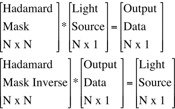
Hadamard Mask N x N

* Light Source N x 1

= Output Data N x 1

Hadamard Mask Inverse N x N

* Output Data N x 1

= Light Source N x 1

A Hadamard mask with 7 elements 0 1 0 1 1 1 0 1 0 1 1 1 0 0 0 1 1 1 0 0 1 1 1 1 0 0 1 0 1 1 0 0 1 0 1 1 0 0 1 0 1 1 0 0 1 0 1 1 1

will modulate a light source with intensities as shown below with respect to space.

8 7 6 5 4 3 2

Multiplexing the light with respect to the Hadamard mask will create the following

= 19 23 20 24 21 18 15 8 7 6 5 4 3 2 * 0 1 0 1 1 1 0 1 0 1 1 1 0 0 0 1 1 1 0 0 1 1 1 1 0 0 1 0 1 1 0 0 1 0 1 1 0 0 1 0 1 1 0 0 1 0 1 1 1 .

The original light source data can be reconstructed. The inverse of the S-matrix used is

= -0.25 0.25 -0.25 0.25 0.25 0.25 0.25 -0.25 -0.25 0.25 0.25 0.25 -0.25 0.25 --0.25 0.25 0.25 0.25 -0.25 -0.25 0.25 0.25 0.25 0.25 -0.25 -0.25 0.25 0.25 -0.25 0.25 -0.25 -0.25 0.25 -0.25 0.25 0.25 -0.25 -0.25 0.25 -0.25 0.25 0.25 -0.25 -0.25 0.25 -0.25 0.25 0.25 0.25 0 1 0 1 1 1 0 1 0 1 1 1 0 0 0 1 1 1 0 0 1 1 1 1 0 0 1 0 1 1 0 0 1 0 1 1 0 0 1 0 1 1 0 0 1 0 1 1 1 1

Multiply this by the output data to recreate the optical signal

= 8 7 6 5 4 3 2 19 23 20 24 21 18 15 * -0.25 0.25 -0.25 0.25 0.25 0.25 0.25 -0.25 -0.25 0.25 0.25 0.25 -0.25 0.25 --0.25 0.25 0.25 0.25 -0.25 -0.25 0.25 0.25 0.25 0.25 -0.25 -0.25 0.25 0.25 -0.25 0.25 -0.25 -0.25 0.25 -0.25 0.25 0.25 -0.25 -0.25 0.25 -0.25 0.25 0.25 -0.25 -0.25 0.25 -0.25 0.25 0.25 0.25

shows that the reconstruction of the original example intensities. This example does step

through an ideal Hadamard recover, but it is not realistic because there is no noise. This

along with other physical characteristics will cause the numbers to change slightly.

5.2 Simple correction matrix

A Hadamard imaging system will have error due to noise, but it is the static and

dynamic idealities that will cause the largest corruption of data. These will cause distortions

in the recovered image. Static nonidealities exist if the mask elements are not totally

transmissive when in the “on” state or completely opaque when in the “off” state. Dynamic

nonidealities result if the mask elements cannot switch between their “on” and “off” states

instantaneously. The static nonidealities of the mask cause a change in the intensities of the

peaks while the dynamic nonidealities of the mask may cause the main peaks in the input

be corrected using a rotating mask as in this thesis because each hole in the mask is different.

The static nonidealities can be corrected by simply normalizing all the individual intensity

peaks as shown in Figure 7-3 and 7-6. These peaks can all be made level to give each fiber

an equal intensity reading assuming that the light across each fiber is equal. This can be done

by the following technique.

They system matrix W can be represented by matrix Ws that describes the

encodements scheme and the static nonidealities of the mask. Ws can also be written in

factored form as

Ws = S Ts (5-18)

where S represents the Hadamard matrix scheme and Ts describes the nonideal static

characteristics of the mask. Once Ws and S are defined, Ts can be obtained. Ts will be a

CHAPTER 6

EXPERIMENTAL APPARATUS

6.1 Hardware

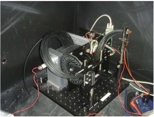
A working prototype model of a Hadamard imaging system was constructed and is

shown in Figure 6-1. A complete parts list of the components can be found in Appendix

A.1. Two design goals of the project were 1) to identify issues with different components

and technical approaches, and 2) keep the size of the device relatively small.

Figure 6-1: Hadamard imaging system constructed

To place limits on the size of the project the rotating mask was limited to the size of a

standard CD which is approximately 4 inches in diameter. The other size goal was to fit the

system on a 1ft x 1ft optical board.

The basic idea of this working model is as follows. A light source will be present

with bioluminescent tumors. This tube will have the ability to rotate by a stepper motor

which will allow for a 360-degree image to be taken. The light from the tube will be coupled

into fiber optics and transported to the mask where the light will be encoded. The encoded

light will then couple to another set of fibers that transport the light to a single photodetector

where intensity of the encoded light will be measured. The mask will then rotate by the

stepper motor to the next position until all the proper combinations of the encoding have

been obtained. Then the tube will rotate to the next imaging position. The process then

repeats until the test object has been rotated by 360 degrees.

While several different methods for making the rotating mask were considered.

Using a printed circuit board manufacturer to drill holes in the board was the method that was

used. A state of on (1) will be created by a hole while a state of off (0) will be made by not

having a hole. Fiber mounts will be made in similar fashion also using circuit boards.

6.1.1 Motors

Two identical stepper motors were accessible at the beginning of this project. Each

motor had a single step turn of 1.8 degrees, making the motor have 200 turns for a complete

360-degree rotation. With the motors, there was the required stepper motor drivers and the

12V, 500mA power supply to drive both motors. Having precision stepper motors such as

these allowed us to step between Hadamard patterns while still maintaining alignment.

6.1.2 Optical fibers

Before any mask or optical mount could be created the type and number of optical

that the most light will couple into each fiber. The choice of using relatively large plastic

multimode fibers instead of the standard 125µm glass multimode fibers was made. This

significantly reduced the complexity of the project when it came to holding the fibers in

position. Important characteristics of these plastic fibers are shown in Figure 6-2. The full

specifications of the fibers used can be found in Appendix A.2. The main features of these

optical fibers were the 1mm core diameter and the angle of acceptance of 27 degrees. This

allowed for lots of modes to easily couple into the fiber. With the plastic fibers, it is even

easy to see room lighting couple into the fiber. The other issue was holding the fibers and

fiber preparation. The 1mm diameter allowed the fiber holders to be constructed in a

straightforward manner. The fibers were relatively stiff compared to optical fibers, but this

also meant they were less susceptible to bending losses.

Core Diameter 1mm

Core + Jacket Diameter 2.2mm

Core Refractive Index 1.49

Clad Refractive Index 1.42

Numerical Aperture 0.46

Figure 6-2: Plastic fiber characteristics

The exact efficiency of coupling the light from one plastic fiber to another via the

mask is unknown at this point, and is dependent on the precision of the alignment. Several

experiments were performed to ensure good alignment between the mask and fibers, but in

general using 1mm fibers rather than 0.0625mm core glass fibers was a big help in

maintaining relatively good coupling. Another reason the large fibers were embraced was

because the core diameter is large enough to be duplicated by a drill bit. With a fiber the size

of a commonly sized drill bit and easily handled by a CNC machine, patterns of holes can be

6.1.3 Hadamard pattern, number of elements

Now that size of the fiber was established along with the size limitation of the mask,

it was apparent that the largest Hadamard matrix that could easily be implemented would be

one of 32 elements since only matrices with 2n elements were considered. A greater number

of elements would not fit on a 4-inch diameter mask. The first row of the 31 element

S-matrix is,

1101101111000101011100001001001

while the rest of the matrix was established by cyclic extrapolation as discussed in Chapter

6.1. The entire matrix is obtained by shifting the previous row one place to the left with any

overflow from the left coming in on the right (Appendix A.3). A “1” will be transferred to

the mask as a 1mm hole (transparent element), while where there is a “0” there will not be a

hole (opaque element).

6.1.4 Mask and fiber mounts

The circuit board program “Eagle Soft” was used to layout all the holes necessary for

the mask and mounts combining the physical properties of the fibers and motor, along with

the 4-inch diameter limitation a rotating Hadamard mask designed. There are numerous

ways the holes in the mask could be arranged. Thirty-two 1mm holes with space in between

each hole to compensate for the fiber jacket diameter were fit into a 10.8-degree pie shaped

area of the circle. It is important to notice that 10.8 is a multiple of a single step of the motor

1.8 degrees. This created 33 (360/10.8) different 10.8 “pies” within the mask circle leaving