High Resolution Environmental Modelling Application Using a Swarm of Sensor Nodes

(1)

High Resolution Environmental

Modelling Application

Using a Swarm of Sensor Nodes

Ferry Susanto

College of Engineering and Science

Victoria University

This dissertation is submitted for the degree of

Doctor of Philosophy

(2)

(3)

(4)

(5)

Declaration

I, Ferry Susanto, declare that the PhD thesis entitled “High Resolution Environmental Modelling Application Using a Swarm of Sensor Nodes” is no more than 100,000 words in length including quotes and exclusive of tables, figures, appendices, bibliography, references and footnotes. This thesis contains no material that has been submitted previously, in whole or in part, for the award of any other academic degree or diploma. Except where otherwise indicated, this thesis is my own work.

(6)

(7)

List of Publications

The following are publications of work undertaken as part of this thesis:

1. Title : Design of Environmental Sensor Networks Using Evolutionary Algorithms

Authors : Ferry Susanto; Setia Budi; Paulo de Souza; Ulrich Engelke; Jing He

Journal : IEEE Geoscience and Remote Sensing Letters IF 2015 : 2.228

Date : 26 February 2016

doi : 10.1109/LGRS.2016.2525980

2. Title : Spatiotemporal Interpolation for Environ-mental Modelling

Authors : Ferry Susanto; Paulo de Souza; Jing He Journal : MDPI Sensors

IF 2015 : 2.033

(8)

viii

I also co-authored the following works during the progress:

1. Title : Visual Assessment of Spatial Data Interpo-lation

Authors : Ulrich Engelke;Ferry Susanto; Paulo A. de Souza Junior; Peter Marendy

Conf. : Big Data Visual Analytics (BDVA), 2015 Date : 22-25 September 2015

doi : 10.1109/BDVA.2015.7314305

2. Title : A Visual Analytics Framework to Study Honey Bee Behaviour

Authors : Engelke U, Marendy P,Susanto F, Williams R, Mahbub S, Nguyen H, and de Souza P Conf. : Proc. of IEEE International Conference on

Data Science Systems (DSS), Sydney Date : December 2016

doi : 10.1109/HPCC-SmartCity-DSS.2016.0214

3. Title : In Search for a Robust Design of Environ-mental Sensor Networks

Authors : Setia Budi, Ferry Susanto, Paulo de Souza, Greg Timms, Vishv Malhotra and Paul Turner Status : Accepted - Environmental Technology Date : 18 Mar 2017

(9)

ix

List of work-in-progress publications:

1. Title : Inferring Apis melliferaBehaviour from Population Activ-ity

Authors : Ferry Susanto, Thomas Gillard, Paulo de Souza, Benita Vin-cent, Setia Budi, Auro Almeida, Gustavo Pessin, Helder Arruda, Raymond N. Williams, Ulrich Engelke, Peter Marendy, Pascal Hirsch

Status : Manuscript completed - Elsevier, Ecological Modelling

2. Title : Data-driven Field Simulation and Environmental Mod-elling for Swarm Sensing Project

Authors : Ferry Susanto, Paulo de Souza Jr., Raymond Williams, Thomas Gillard, Setia Budi, Peter Marendy

Status : Manuscript completed - IEEE Transactions on Geoscience and Remote Sensing

3. Title : Agent-based Modelling of Honey Bee Forager Flight Be-haviour for Swarm Sensing Applications

Authors : Paulo de Souza, Raymond Williams, Stephen Quarrell, Se-tia Budi, Ferry Susanto, Benita Vincent, Geoff Allen, Auro Almeida, Dale Worledge, Leandro Disiuta, Pascal Hirsch, Gus-tavo Pessin, Helder Arruda, Peter Marendy, Leon dos Santos, Tom Gillard, Andojo Ongkodjojo Ong

Status : Under review - Environmental Modelling and Software

4. Title : Design of Environmental Sensor Networks with Support of Mobile Platform

Authors : Setia Budi, Paulo de Souza, Greg Timms,Ferry Susanto, Vishv Malhotra and Paul Turner

(10)

x

5. Title : Low-Cost Electronic Tagging System for Bee Monitoring

Authors : Paulo de Souza, Benita Vincent, Stephen Quarrell, Gustavo Pessin, Setia Budi,Ferry Susanto, Geoff Allen, Peter Marendy, Auro Almeida, Dale Worledge, Pascal Hirsch, Leandro Disiuta, Ulrich Engelke, Huyen Nguyen, Raymond Williams

(11)

Acknowledgements

This project would not be possible without the support of many people. First of all, this thesis is dedicated to my parents, who have unconditionally supported and encouraged me. I would like to thank a number of institutions that have financially supported my study: (i) Victoria University for waiving my PhD tuition fees; (ii) Vale Institute of Technology for the award of a postgraduate scholarship; and (iii) CSIRO’s the Office of the Chief Executive program for a top-up scholarship. This wonderful support has allowed me to fully focus entirely on my PhD work.

I express my deepest gratitude to my supervisors: Prof. Jing He (Victoria University, Melbourne), Prof. Paulo de Souza (CSIRO), and Guang Yan Huang (Deakin University), for the continuous support and guidance that they have offered throughout the PhD progress, as well as for their patience, enthusiasm, encouragement, and knowledge. Their feedback on the research work and the thesis writing have contributed greatly to the success of this work.

I would also like to thank CSIRO for providing four different data sources to allow the development and experimental simulation possible, they are: (a) a ‘modelled’ Environmental data of the South Esk region, in Tasmania; (b) a ‘benchmark’ data set that collects envi-ronmental observations from a number of weather stations at South Esk region; (iii) an agent-based bee flight simulator developed by the Swarm Sensing team; and finally (iv) real bee experimental data using RFID-based systems conducted at Geeveston, Tasmania.

(12)

(13)

Abstract

The advancement of sensing technology has successfully reduced the physical size of a sensor node and stimulated the application of swarm sensing (millimetre scale sensors). Such a system has been envisioned to provide novel applications. For example, CSIRO has commenced the application of swarm sensing technology to track insect that aims to understand how the environmental situation influences bee behaviour.

While the micro-sensor is still under development, it is crucial to have a baseline data set for initial data analysis purposes so that reasoning with the rich data is possible once the hardware has been developed and deployed. This work will propose a field simulation to address this issue. A hybrid environmental sensor network will be deployed, for the purpose of making highly dense observations, that consists of: (i) fixed sensor nodes, acting as weather stations, that collect data in a regularly-spaced time interval; and (ii) mobile nodes that sense the environmental parameters while insects move within the region with extremely high frequency – i.e. seconds.

The proposed spatio-temporal interpolation algorithm in this dissertation (i.e. for environ-mental modelling) has achieved a computational efficiency factor from highly-dense sample data with an acceptable statistical error. The method also reconstructs the environmental situation in reality – e.g., produce a smooth surface in space and over the time.

(14)

(15)

List of figures

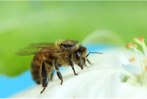
1.1 An example of a bee with a Radio Frequency Identification (RFID) micro-sensor (2.5mm × 2.5mm × 0.4mm, 5.4mg) mounted on its thorax. Credit: CSIRO. . . 2 1.2 An illustration of sensor networks to be developed within the SSP: (a)Sensor

nodes. An individual sensor that records environmental data, i.e., bees in this case; (b)Base station. Infrastructure acting as an “agent” that receives values from individual sensor nodes and sends them to the database to be stored; (c)Database. A medium that records the raw data collected, which always comes with a periodic backup system for security purposes. . . 3

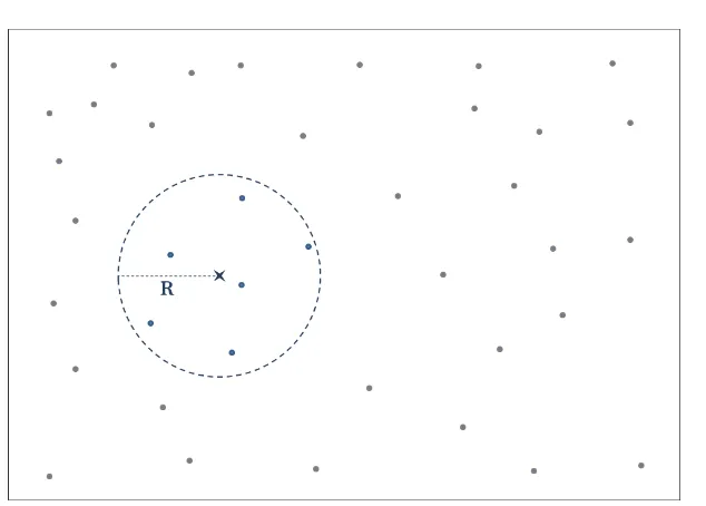
2.1 A demonstration of the improved IDW. The dots are the sample data points, and the ‘×’ is the point location to be interpolated. Ris a user-defined radius parameter that indicates the farthest distance to be included from the point×. On this case, only a total of six sample points will have an influence on the interpolation process. However, no empirical approach has been developed to obtain the optimal value for the parameterR. . . 13 2.2 An illustration of the TIN interpolation technique for pointxthat lies within

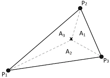
a triangle formed by pointsP₁,P₂, andP₃ (holding values ofv₁,v₂, andv₃ respectively). The weight for each point is calculated based on the corre-sponding area; for instance,P₁has the weight A1

A (whereA=∑ N=3

i=1 Ai) and

so on. . . 17

(20)

xx List of figures

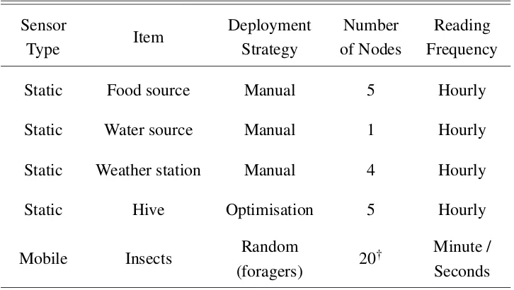
3.2 An overview of the swarm sensing field simulation to produce highly-dense observations (Section 3.4) to be utilised as an input for the spatio-temporal interpolation algorithm (Section 3.5). Spatial sampling to optimise the hives locations (Section 3.2) and modelling bee behaviour (Section 3.3) are acting as the “supporting components” in order to accomplish the field simulation. 28 3.3 A typical surface height data visualisation of Tasmania’s South Esk

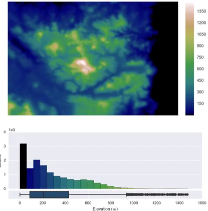
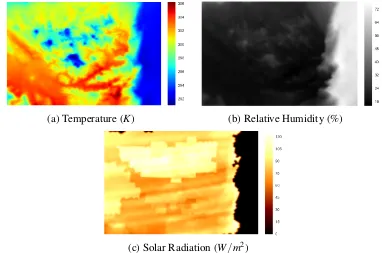
Hy-drological model: (top) The actual elevation data (meters) within the RoI; (bottom) The distribution of elevation values within the 151×101 grid. . . 30 3.4 Example of three environmental parameters that are utilised in this work: (a)

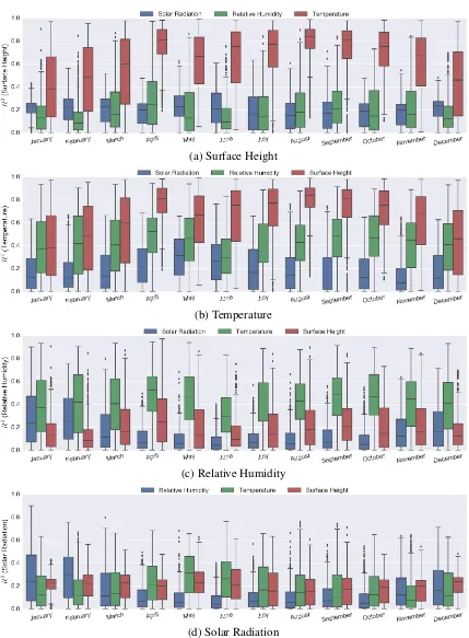
temperature; (b) relative humidity; and (c) solar radiation. The colour bar on the right of each image corresponds to each parameter’s value and unit. . . 32 3.5 Box plot demonstrating the monthly R2 value of hourly data (2-D map)

between parameters throughout the year 2013. The horizontal axis represents the months in a year and the vertical axis shows the correspondingR2value. 33 3.6 A snapshot visualisation of the output generated by the agent-based

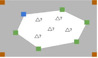
compu-tational bee foraging flight paths. . . 34 3.7 Illustration of the ‘convex hull’ generated bySN_{f ood}∪SN_water (white area),

in which the SN_hive is allowed to be optimised within. The squares are: weather stations at the map’s corners (brown), food (green) and water (blue) sources respectively; whilst the triangle denotes the locations of bee hives to be optimised. . . 36 3.8 A chromosome encoding and decoding example that consists of only the

hive nodes which are to be optimised. . . 37 3.9 An illustration of the chromosome design utilised in this work, where each

element within the individual holds a value between 0 and 1, andBdenotes the background (BKG). The encoding and decoding example of the intensity (I_i)parameter of distributionG_iis also presented. In this case, assume that we have elementI_iwith value 0.7615 (encoded) within the individual which is equivalent to 205.32 (decoded) after applying Equation 3.12. . . 43 3.10 Simulation procedure to generate an artificial bee. . . 44 3.11 Data pre-processing (spatial-only case). Left: 2D spatial map; Right:

’parti-tioned’ sub-area from the map. . . 51 3.12 Data pre-processing for 2D-spatial + 1D-temporal case. Left: 3D

(21)

List of figures xxi

3.13 Visual illustration of the proposed STI algorithm. In this example, the value at timet is to be interpolated. The algorithm first estimates the values at both t_lo=t2 (red) andthi=t3 (blue) utilising the extension approach (Equation 3.23); and then interpolates the value at timet (purple) using the reduction approach (3.22). . . 53 4.1 Demonstration of the EA-assisted ESN optimisation: (a) the RoI and the

pre-defined static nodes for execution; and (b) using the number of hives to be optimisedN=N(SN_hive) =5. The figure is labelled as follows: red square (SNcorner), green square (SNf ood), blue square (SNwater), yellow triangle

(SNhive), and the ‘convex hull’ area (dashed-line connecting nodes: SNf ood∪

SN_water) within whichSN_hive are to be optimised.. . . 59 4.2 Visual examples for the optimised sensor nodes (yellow triangles) within the

RoI bounded by the map’s corners (red squares). . . 60 4.3 Computational efficiency comparisons between distinct methods. The

fig-ure demonstrates the mean and its corresponding 95% confidence interval (vertical bar). . . 61 4.4 RMSE comparison of elevation data between different interpolators. . . 62 4.5 Visual assessment of different interpolators using the optimised sensor nodes

and the interpolated/estimated surface height data based on the design shown in Figure 4.2. Each row represents a different method and each column a different number of nodes. . . 62 4.6 Raw daily detections data from the bee experiment at Geeveston, Australia. 65 4.7 Bee behaviour data after applying the bee classification rules as described

in Section 3.3.1. These data will be used for the curve fitting optimisation process to be applied later. . . 65 4.8 Bee activities duration from the data in Figure 4.7. . . 66 4.9 Outcome of the curve fitting process for different bee behaviours. The dots

represents data and the solid-line denotes the curve fitted Gaussian PDF. Note that the black dots and black dashed-line denote the summation of data (D) and Gaussian PDF (GALL), respectively. . . 67

4.10 Normalised values (presented as percentages), based on Figure 4.9, of bees involved in different activities relative to the time-of-day. . . 67 4.11 An illustration of the sampled data (CSV output file) from the swarm sensing

(22)

xxii List of figures

4.12 A demonstration of the field simulation, showing the data collected within the RoI (X and Y spatial dimension) throughout the day (Z - time of day). Squares denote hourly data detections from the static sensor nodes: food (green) and/or water (blue) sources, the weather stations at the map’s corners (red). Triangles are the hives that are represented using different colours. Finally, the arrows represent bees’ flight paths and each of them is a particular datum obtained by ‘sensing’ the environment. Flight paths of a particular colour match the colour of the hive from which that bee originated. . . 70 4.13 A dashboard illustrating the data obtained from the proposed field simulation

framework. The left pane represents the time-line throughout the day for a single bee simulated from distinct hives, and includes the following compo-nents: (a) hourly data collected from each hive. (b) simulated bee activity in that day and its corresponding duration; (c) high-resolution data generated by ‘sensing’ the environment from mobile sensor nodes. The right pane is a top-down view based on Figure 4.12, that disregards the temporal dimension (time-of-day). . . 71 4.14 Spatio-temporal empirical variogram model generated using the static-only

nodes for the temperature data on 06 January 2013. . . 72 4.15 High resolution data obtained from the Swarm Sensing hybrid sensor network

(Section 4.3). Each dot is a data point ‘sensed’ by either a fixed or a mobile node. The data are denoted using different colours based on time-of-day (z-axis): early morning (00:00, blue); noon (12:00, red); and late night (24:00, green). . . 73 4.16 Visualisation of the data set after the ‘pre-processing’ procedure. Each dot

representing data holds the mean (µ) and the standard deviation (σ) value

that will be used for the interpolator’s estimation and its corresponding error, respectively. . . 74 4.17 Scatter plot based on Table 4.3: x-axis denotes the sites, and y-axis is the error

values for corresponding error measurements (i.e. Pearson’sr, MAE, and RMSE). The shapes are used to distinguish theScheme: square (Scheme 1), triangle (Scheme 2) and cross (Scheme 3); The colours represent distinct parameters: temperature (green), relative humidity (blue), and solar radiation (red). . . 75 4.18 Timeline plot showing the values from three different data sets: ‘benchmark’

(23)

List of figures xxiii

4.19 A visualisation demonstrating the ‘modelled’ (left) and ‘estimated’ (right) temperature data on 06 January 2013. It also presents the spatial locations of six weather stations (denoted using ‘×’) from the ‘benchmark’ data set. . . 77 4.20 Demonstration of high-resolution spatio-temporal environmental modelling.

(24)

(25)

List of tables

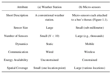
3.1 Distinct types of sensor nodes to be deployed: (a) static weather station; and (b) mobile micro-sensors.N indicates the number of sensor nodes. . . 26 3.2 This table shows the configuration of the field simulation to be deployed

within the area of interest (South Esk region of Tasmania, see Figure 3.1). . 27 3.3 List of data set notations and abbreviations that will be used throughout the

dissertation. . . 29 3.4 Sites information that was utilised as the ‘benchmark’ data set. Note that

within the ‘Parameters’ column, the following abbreviations are used: temp (temperature), rh (relative humidity), and rnet (solar radiation). . . 35 3.5 Summary of bee activity classification rules based on field observations.

Within the ‘Activity Duration’ column, if the durationx is more than the pre-determined range (e.g., by the entryx>30m), the data will be omitted. Note that the configurations may vary for different bee species. . . 39 3.6 Mathematical notations that will be used throughout this sub-section. . . 41 3.7 The empirical rules utilised for choosing the next activity (anext) of a bee

based on its current activity (acurr). TheInit denotes that thetcurr is the first

detection (detectionf irst) of that particular bee on that day. . . 45

3.8 Data sampling configuration for mobile sensor nodes – insects. Note that the ‘· · ·’ on row ‘Detections’ indicates that the data are collected continuously with a certain interval (column ‘Frequency’) between the start and end time-in-day. . . 47 4.1 EA parameter configuration to be utilised within the execution. . . 59 4.2 Parameter details for the curve fitting results shown in Figure 4.9. The

(26)

xxvi List of tables

5.1 Summary comparison of interpolators. The values are to be interpreted as: +1(most preferred),0(neutral), and-1(least preferred). . . 82 5.2 Summary of bee behaviour with the ‘possible’ activities for each

(27)

Chapter 1 Introduction

1.1 Background

Wireless sensor network is a set of interconnected sensor nodes deployed with the purpose of observing environmental conditions such as temperature, relative humidity, solar radiation. Such a system has become the key technology for the future of environmental monitoring, allowing us to observe environmental variables at difficult and hostile locations such as mountainous and deep marine region. This technology offers a significant contribution to our society, for instance, early warning system, weather forecast, and precision agriculture. However, the deployment of those fixed sensor nodes (e.g., weather stations) offer a low spatial coverage. Also, it requires an appropriate deployment strategy (also known asspatial samplingmethod) to obtain a cost-effective and a fit-for-purpose network (i.e., a required level of network representativeness).

A mobile sensor node, on the other hand, is more versatile than fixed sensor node. It makes observations while it moves through the area under study (e.g., aerial and autonomous underwater vehicle). It suffers from the limitation of having a small temporal coverage at discrete locations. With the advancements in the sensor technology, the cost and size of an individual sensor node have been decreased. For instance, the Smart Dust project [1] was envisioned to provide thousands of millimetre-scaled sensing with high spatial and temporal coverage (also known as swarm sensing). Such a network provides much more discrete measurements of the environment in a less intrusive way. Example applications using such a technology could be found in the military (e.g., unmanned aerial vehicles) and animal (or even insect) tracking.

(28)

2 Introduction

a continuous surface of the region under study, in which able to support a more accurate interpretation and decision making. Nonetheless, choosing a suitable interpolation method is a non-trivial task, and an in-depth investigation must be carried out for the applications in different purposes. This is because the performance of any interpolator can vary based on different data sets and requirements (e.g., accuracy and computation efficiency).

1.2 Motivation

CSIRO (Commonwealth Scientific Industrial Research Organisation) has commenced the development of the swarm sensing technology that attaches micro-sensor to insects (bee in this case). Such a configuration allow the mobile sensor nodes to make observations as the bees moving throughout the Region of Interest (RoI). As a result, highly dense data sample will be obtained, this has stimulated the demand for a computational method to process and visualise a large amount of data and to make sense of them. CSIRO’s Swarm Sensing Project (SSP) aims to better understand bees’ response to different stressors such as environment (e.g., strong wind, heavy rain, extreme weather, pollution) and the surroundings they are experiencing in (e.g., pesticide exposure, varroa mites, human intervention).

Fig. 1.1 An example of a bee with a Radio Frequency Identification (RFID) micro-sensor (2.5mm × 2.5mm × 0.4mm, 5.4mg) mounted on its thorax. Credit: CSIRO.

(29)

1.2 Motivation 3

utilise computational techniques to infer bee behaviour at colony level so that we can answer the following question: what is the probability of an individual bee in the colony to forage at a particular time of day (e.g. 6am, 1pm and 4pm)?

Fig. 1.2 An illustration of sensor networks to be developed within the SSP: (a)Sensor nodes. An individual sensor that records environmental data, i.e., bees in this case; (b)Base station. Infrastructure acting as an “agent” that receives values from individual sensor nodes and sends them to the database to be stored; (c)Database. A medium that records the raw data collected, which always comes with a periodic backup system for security purposes.

Figure 1.2 illustrates the sensor network design to be developed within the next phase of the SSP. The design consists of three components: (i)sensor nodesacting as individual entities scattered throughout the region to sense the environment; (ii) a base station that collects the data obtained from the sensors; and (iii) adatabaseto store the data collected from the networks.

In the Swarm Sensing project, a number of fixed sensor nodes (such as hive and the weather station) will be deployed within the region of interest to collect environmental data in a specific interval (e.g. 5 minutes, 15 minutes, or 1 hour). Nevertheless, aspatial samplingalgorithm is needed to obtain a set of representative locations depending on the number of weather stations to be deployed. On the other hand, the mobile sensor nodes are being attached to insects to collect environmental data as they move within the landscape. However, while the development of micro-sensor is still being undertaken and rich data set is not available as yet, and so this dissertation also proposes a framework that generates high-resolution irregularly spaced data points to allow initial statistical data analysis.

(30)

4 Introduction

area under study, interpolation and extrapolation of missing values is critical to estimate the value at locations without data sampling. Therefore, this dissertation proposes a suitable spatio-temporal interpolation algorithm to accurately model the environmental situation within the RoI.

1.3 Research Objectives

The main objective of this thesis is to develop a near-to-reality Swarm Sensing Project field simulation framework and high-resolution environmental modelling within a small-scaled RoI. This work focuses on the following research components to achieve the objective:

1 To propose aspatial samplingalgorithm to obtain representative locations for a set of static sensor nodes under the study region;

2 To propose a data-driven modelling to infer bee behaviour at the colony level;

3 To propose a Swarm Sensing field simulation framework to generate high-resolution observations (data sampling) within the region of interest from fixed (weather stations) and mobile (insects) sensor nodes.

4 To propose a spatio-temporal interpolation that suits the purpose for swarm sensing applications, based on the following factors: able to incorporate huge amount of data, low estimation error, and to create a smooth surface that accurately represents the real environmental situation.

1.4 Thesis Structure

(31)

Chapter 2 Literature Review

A comprehensive overview of current technologies relating the objectives of this dissertation will be presented in this chapter. As discussed in Chapter 1 (Introduction), the ultimate goal of this work is the construction of a close-to-reality environmental model using data acquired from hybrid (static and mobile) sensor networks (Section 1.3). As such, this chapter will be partitioned into three major themes: (a) environmental sensor networks and their deployment; (b) computational insect behaviour modelling; and (c) spatial and spatio-temporal interpolation techniques. A summary discussion on how each component would contribute to this work (i.e. the swarm sensing simulation framework in Chapter 3) will be reported at the last section.

2.1 Environmental Sensor Networks (ESN)

The environmental study is an important area that provides a better understanding of natural situation and also offers a significant contribution to our society. The collected data from the sensor network is crucial for environmental managers to support decisions for an effective use of natural resources for other significant applications of benefit to our society (e.g. hazard warning services). Institutions that provide warning services often do not have enough quality data (regarding spatial and temporal coverage) that can be used to support highly accurate predictions [2–4]. Therefore, ongoing enhancement of the system’s components (i.e. sensor nodes, communication engineering, power management, stability, security) is a demanding task. Hart and Martinez (2006) have provided an extensive review of ESN usage examples and they also envisioned that ESN could become a standard research tool in the near future [3].

(32)

6 Literature Review

control, industrial automation, and environmental monitoring [2, 3, 5]. It combines sensing, communicating, and computing capabilities (e.g., hardware, software, and algorithms). Such systems evolved from being passive logging systems (involving human-exhaustive effort, i.e. system maintenance and data collection) to ‘intelligent’ networks, where advances in cyber-infrastructure have driven the need for better sensor networks to suit different needs for designated applications or research studies. For example, enhancements in electronic miniaturisation and for wireless technologies over past decades have opened up the following unprecedented opportunities [4, 5]: (a) Making measurements at previously inaccessible and dangerous locations; (b) Improving the data quality in terms of spatial and temporal scales; (c) Obtaining unexpected observation results that led to the development of new paradigm; (d) Collaborating work between researchers across distinct professions.

An understanding of the following ESN components is required [2–6] prior to building a fit-for-purpose sensor network:

i The purpose of the sensor network. This includes the form of data collected and its interpretation, which has a significant effect on the entire design of the system network (e.g. communication technologies, security).

ii Technological capabilities and the physical environment.This relates to the deployment feasibility of sensor network, such as in mountainous or deep marine regions; and the hardware’s ability to withstand hazardous situations.

iii System standardisation and usability.Variations in data format, hardware and software design cause difficulties in interoperability, especially when the system requires consid-erable amount of technical knowledge to be operated and maintained by professionals from different backgrounds.

iv Other sensor node design goals, including types of data (e.g. use of biotechnology), sensor integration, size, robustness, power management.

Spatial samplingmethods in ESN deployments make an effort to locate sensor nodes in a way that meets desired design goals [6]. Those methods have attracted wide interest in the ESN deployments research area. The following sub-sections investigate the different types of spatial sampling and discuss the swarm sensing requirements for ESN design application.

2.1.1 Sampling with Fixed Nodes

(33)

2.1 Environmental Sensor Networks (ESN) 7

requirements. It has been categorised as an NP-hard (non-deterministic polynomial-time hard) problem [6, 7], where heuristic-based approaches (mathematical programming) have been extensively used to address this problem.

Evolutionary algorithms have been utilised to optimise the sensor node placement for distinct purposes [8–12]. This technique has been widely used for optimisation mainly owing to its capability for solving multi-objective problems, where a set of near-optimal solutions (the Pareto Front, PF) will be generated as the result. In some cases, the network manager is required to possess a certain level of domain knowledge to select a particular solution from the PF [10] by considering other factors, such as the desired network’s sparsity level or the feasibility of the sensor node deployments. In addition, spatial simulated annealing has also been utilised in several studies [13–17] and proven to be practical for spatial sampling purposes.

Despite the variety of optimisation techniques used for ESN deployments, the literature has reported a wide range (yet similar) of design goals. The aspects that are most-discussed and incorporated within the WSN deployment process [6]: (i) network lifetime [7, 18, 19]; (ii) connectivity [17–20]; (iii) coverage [19, 21]; (iv) relay count [19, 20]; (v) data fidelity [21, 22]; and other aspects such as cost, energy, and minimal sensor counts [7, 11, 17, 19, 21, 22].

2.1.2 Sampling with Mobile Nodes

(34)

8 Literature Review

2.2 Social Insect Modelling

This section reviews relevant topics regarding social insect behaviours (with particular an emphasis onApis mellifera, the European honeybee). The following review includes honey bee behaviour (i.e. bee’s foraging roles) and computational bee modelling applications. These components are crucial because one of the major contributions in this dissertation is to propose a swarm sensing field simulation, using insects as the mobile sensor nodes (bee in this case), to generate a highly dense data points in the region under study.

2.2.1 Bee Foraging Roles

The development of honey bee foraging can also be broken into several distinct roles depend-ing on the bee’s age and its knowledge of profitable food resources [29]. Initially, novice bees make several orientation flights to familiarise themselves with the landscape around the hive [30]. Such effort is crucial for successful homing after future foraging activities. Over time, bees may start to spontaneously search for food sources. These bees can be seen as ‘scouts’ as they are effectively naive to the availability and/or proximity of food resources in their foraging range [31]. Alternatively, the same bee whilst in the hive may observe a waggle dance, and utilise the positional information gleaned from the dance to locate food resources located by other scouts, and there-by become a ‘recruit’ [32–34].

Once the food source is found, the bee shifts to become an ‘exploiter’. It remembers the exact location of the source, flying backwards and forwards between the hive and the source to retrieve nectar, pollen, and/or water until the source becomes exhausted or the hive’s needs change. During this time, the bee may perform the waggle dance to inform other bees of the source’s profitability and location [35].

Bees will cease exploiting the resource once it is exhausted, and may either become restingforagers or perform reconnaissance flights (as an ‘inspector’) to examine whether the source has replenished and, if so, will start exploiting it again [36]. Alternatively, they may start to scout for unknown resources or observe waggle dances to again become a recruit. As a bee becomes more experienced, it tends to retain a constant trip duration but with much faster speed and larger area coverage [30].

(35)

2.2 Social Insect Modelling 9

2.2.2 Computational Modelling of Bee Behaviour

Numerous attempts have been made to model both in-hive and out-of-hive bee behaviours. Pirk et al. have provided a comprehensive review of statistical guidelines for in-hive bee experimental design [38]. They have concluded that parametric testing (i.e. regression, normal distribution) and multivariate analysis (i.e. principal component analysis) are suitable methods for data analysis purposes (statistical inference) in bee research.

A recent study proposed an algorithm to post-process bee experimental detection data, to reconstruct bee foraging behaviour, collected from RFID (Radio-Frequency Identification) tags with a reader installed at the hive and feeder entrances [39]. When developing this ‘Track-a-forager’ algorithm, two major issues needed to be addressed prior to data analysis: (a)rapid-successionscans where successive detections were recorded in a very short time interval; and (b)missed readingsmainly caused by the hardware limitation including small tag sizes leading to low detection ranges. Despite these issues, the ‘Track-a-Forager’ program has been successfully developed and is appropriate for analysing foraging bee behaviour based on the assumption that the minimal foraging duration is five minutes.

Vrieset al.modelled individual bee foraging behaviour by considering the in-hive com-munication between foragers to investigate the parameters that influence foraging behaviour in a bee colony [31]. The motivation for this simulation was the fact that food profitabil-ity information encoded in the bee’s waggle dance has a substantial influence on foraging behaviour at colony level [36]. It is also found that the food source positional information and the probability of a bee abandoning an exhausted source are important factors when developing an accurate foraging model. For this reason, Granovskiyet al. used both field experiments and a mathematical model to demonstrate the influence of the waggle dance on bee foraging behaviours at a colony level on both short and long timescales [36].

An out-of-hive foraging simulation has also been proposed by Adeva to model bee foraging behaviours during food resource depletion and replenishment [40]. This model also incorporated distinct weather parameters in its final version. The simulations generated lacked benchmark behavioural data, making it impossible to validate the model and therefore validating the accuracy of the system.

(36)

10 Literature Review

Application of these technologies to the problem of colony collapse disorder will not only help to further the development and improve the application of technology, but will also serve to assist in solving the crisis facing bee populations. Use of the technologies in this setting allows for field testing of ESNs and improvement of these devices. The data gathered during these experiments will also allow for monitoring of honey bee colony health, providing baseline data, and colony health can also be manipulated using commonly applied chemicals, for instance, to test their effects on bees in the field, furthering research into bee health and disease investigations.

2.3 Interpolation Algorithms

Interpolation is a method that is used to estimate any unknown values within known points. For example, given a set of data points/valuesV ={v₁,v₂,v₃,· · ·,v_i,· · ·,v_N}atN-locations based on a function f(x), for which we do not have an analytical expression of this function. The aim of an interpolation method is to construct the original function f to estimate any arbitrary spatial locations.

Interpolation is a crucial process where we want to get the information about meaningful values in the area of interest and has been widely used in many disciplines. It plays a critical role in the environmental sciences, because of the fact that the environmental analyst requires spatially continuous data over the area of interest to make valid and confident judgements.

The list below summarises the theoretical features associated with interpolation tech-niques [41]. Understanding these characteristics is crucial for the environmental manager because of the fact that there is no single interpolator that suits every situation. A thorough investigation is required to select the ‘best suited’ method for a particular purpose.

- Global versus local.Global methods utilise the entire observation sample for estimation to capture the general trend. Local methods, on the other hand, only considers the samples within a specified distance from the point to be estimated and so are capable of capturing the local variance [42].

- Exactness. This element is determined by whether or not the method will estimate the same value at sampled locations. Some examples of an ‘exact interpolator’ are the nearest neighbour (NN) and triangulation irregular network (TIN) methods [41]. In addition, some statistical error measurements (e.g. leave-one-out cross-validation) adopted the ‘exactness’ feature to determine the quality of ‘inexact interpolators’ [42]. - Deterministic versus stochastic. A stochastic method provides an estimation of the

(37)

2.3 Interpolation Algorithms 11

- Gradual versus abrupt. This defines the smoothness of the estimated continuous surface produced. Gradual methods generate smooth and gradual changes between the sample observations; In contrast, an ‘abrupt’ technique (i.e. nearest neighbour interpolation) will produce sharp boundaries in the interpolated surface.

- Convex versus non-convex. A ‘convex’ interpolator will estimate values between the minimum and maximum values of the samples (i.e. min≤estimate≤max). A ‘non-convex’ method, on the other hand, might produce estimations that are lower and greater than the minimum and the maximum values, respectively. An example of such occurrences is in Kriging where some samples could produce negative weighting values resulting from the ‘screen effect’ [43].

- Univariate versus multivariate. ‘Univariate’ methods use only one primary variable (i.e. values at the sampled locations) for estimation, some examples are inverse distance weighting, simple kriging, ordinary kriging, and triangle irregular network. ‘Multivariate’ interpolators utilise more than one variable within the process, for

instance, ordinary cokriging (OCK) and kriging with external drift (KED).

There has been an increased demand for interpolation techniques to incorporate spatio-temporal data. Many efforts have been initiated to address this research problem – the development of Spatio-Temporal Interpolation (STI) algorithm.These adopt either [44, 45]: (a) anextensionapproach – It converts the ‘temporal’ dimension into spatial-distance. On other words, it extends the STI problem into a higher spatial interpolation problem; or (b) areductionapproach – Such a method reduces the STI technique to a regular interpolation problem in a way that it estimates the values using spatial-only interpolation method, and then applies a time-function to incorporate the ‘temporal’ element within the estimation.

The following sub-sections will review some widely-used techniques providing, for each method, a description of both spatial-only and STI algorithms. Finally, a summary of applications and related research using these techniques will be presented.

2.3.1 Inverse Distance Weighting (IDW)

Inverse Distance Weighting (IDW) is one of the most widely used interpolation techniques, proposed by Shepard in 1968 [46, 47]. This technique is categorised as a deterministic method and is based on the assumption that the value to be interpolated is likely to be more similar to the nearer observed values than to those at a greater distance. This technique is expressed in the following:

ˆ

f(x,y) =

N

∑

i=1

(38)

λ(dsi)i=

d−us

si

∑N_i=1d

−us

si

(2.2)

d_s_i=

q

(x_i−x)2_{+ (}_y

i−y)2 (2.3)

where ˆf(x,y)indicates that we are estimating the value at locationx,y;λ(dsi)iis the weighting mechanism;dsiis the spatial distance (2-dimensional Euclidean distance) between the point to be interpolated (x,yin this case) and the known data point (vi);us is a user-defined parameter

that is used to adjust the diminishing strength in relation to increased spatial distance; and,N is the total number of known points. If the configurationus=2 is applied, this IDW becomes

the Inverse Distance Squared technique [48]. Yet, the parameterus need not always be to

two, and can be adjusted to improve performance [49]. The complexity of conventional IDW isO(N)which can be seen from Equation 2.1.

The so-called ‘zero distance problem’ has been discussed by de Mesnard [50]. For the case where location to be interpolated is exactly the same as one of the reference points (i.e. dsi =0), Shepard [46] does not interpolate that particular location because we already have full knowledge at that point – thediscretecase. Unfortunately, such implementations may not be realistic when the mean within a particular area (suburb, city, state, country) is being estimated (i.e.dsi→0) and, for these situations, utilising thecontinuouscase is more satisfactory.

Improved IDW

(39)

Fig. 2.1 A demonstration of the improved IDW. The dots are the sample data points, and the ‘×’ is the point location to be interpolated. Ris a user-defined radius parameter that indicates the farthest distance to be included from the point×. On this case, only a total of six sample points will have an influence on the interpolation process. However, no empirical approach has been developed to obtain the optimal value for the parameterR.

STI - Extension approach

The extension approach to the IDW’s STI method (2-D Space and 1-D Time problem) was described by Li and co-authors in 2014 [51]:

ˆ

f(t,x,y) =

stend

∑

tstart

N

∑

i=1

λ(dsti)st,i·vt,i (2.4)

λ(dsti)st,i=

d−ust

sti

∑N_i d−stiust

(2.5)

d_st_i=

q

(x_i−x)2_{+ (}_y

i−y)2+c2(ti−t)2 (2.6)

(40)

The extension of this approach to the 3-D space and 1-D time problem can be expressed in a slight variation based on Equation 2.6, so that it becomes:

d_st_i=

q

(x_i−x)2_{+ (}_y

i−y)2+ (zi−z)2+c2(ti−t)2 (2.7)

wherezis the 3rd spatial dimension in which always seen as the altitude (surface height).

STI - Reduction approach (ST Product Method)

This method was proposed by Liet al. and is constructed in the following way [45]:

ˆ

f(x,y,t) =

N

∑

i=1

λ(dsi)s,i · fˆ(t) (2.8) ˆ

f(t) = ti2−t t_i₂−t_i₁vi1+

t−t_i1

t_i₂−t_i₁vi2 (2.9) where the spatial weightingλ(dsi)s,iis equivalent to Equation 2.2; ˆf(t)is the estimated value at timet;t_i₁andt_i₂are the first (previous) and second (next) time indices, and similarly,v_i₁ andv_i₂are the first (previous) and second (next) value at corresponding timet.

It is important to note that such an algorithm (Equation 2.9) relies on the assumption that values at the same location (vi1andvi2) but at different times (ti1andti2) are provided. Nevertheless, one of the assumptions of this dissertation is that the data are not necessarily collected in a finely-gridded manner (in both the spatial and temporal dimensions). Due to the fact that this algorithm does not meet the assumptions of this thesis, it will not be considered and applied to the simulation in this work.

2.3.2 Kriging

The Kriging interpolation technique, also called the Kriging esimator, is categorised as a geo-statistical method because it takes the spatial patterns and the uncertainty of the surrounding surface into account during the interpolation process [42]. An observation Z(s,t) can be seen as a combination of a space-time mean componentm(s,t) and a stochastic residual componentY(s,t), written as:

Z(s,t) =m(s,t) +Y(s,t) (2.10)

(41)

and residual), and an example of the Ordinary Kriging (OK) calculation will be provided at the end.

Trend Characterisation

The behaviour of an observation variable is different at different spatial and temporal scales and so can be characterised using a combination of linear models as follows:

m(s,t) =

p

∑

i=0

βifi(s,t) (2.11)

whereβi is an unknown regression coefficient; fi represents the covariates that must be

known exhaustively over the space-time domain; and pis the number of covariates.

Stochastic Residual Modelling – Variogram

Asemi-varianceis generated to show how much a location point is related to its neighbour points within a particular distance (called thelag) by using the following equations for the spatial-only and the spatio-temporal cases:

ˆ

γs=

1 2E

Y(s)−Y(s+hs)2 (2.12)

ˆ

γst =

1 2E

Y(s,t)−Y(s+h_s,t+h_t)2 (2.13) whereEdenotes mathematical expectation;Y(s)andY(s+h_s)is the residual value at spatial locationsands+h_s(separated by spatial lag distanceh_s) respectively. The semi-variance

ˆ

γ(hs)is plotted againsths, and needs to be fitted in order to create the so-calledvariogram

modelfor the estimator process in the later stage.

Some widely-used spatio-temporal stochasticsemi-variancemodels are briefly discussed below:

(a) Sum-metric model. This model is based on the assumption that the three components (spatial, temporal, and spatio-temporal) are mutually independent [52]:

γst(hs,ht) =γs(hs) +γt(ht) +γst

q

h2

s+ (α×ht)2

(2.14)

whereht is the temporal distance lag; and α is the spatio-temporal anisotropy ratio that

(42)

(b) Product-sum model. Proposed by de Iaco [53] in the form of:

γst(hs,ht) =γst(hs,0) +γst(0,ht) +kγst(hs,0)γst(0,ht) (2.15)

with

k= sillγst(hs,0) +sillγst(0,ht)−sillγst(hs,ht) sillγst(hs,0)sillγst(0,ht)

(2.16) wheresillγst(hs,ht)denotes the ‘global’ sill estimated by ‘eye-fit’ after plotting the sample

variogram surface (γst(hs,ht)) or by fitting to minimise the least-squares error of Equation

2.15 [53]. Also, the following must be met in order to satisfy the admissibility condition for k:

0<k≤1/max{sillγst(hs,0),sillγst(0,ht)} (2.17)

Ordinary Kriging (OK) Estimation

The weighting mechanism for the OK estimator is formulated by solving the equation:

A−1·b=

"

λ

φ

#

, A=variogram_model(D_N,N) (2.18)

DN,N=

     

d₁_,₁ d₁_,₂ · · · d₁_,_N d₂_,₁ d₂_,₂ · · · d₂_,_N

..

. ... . .. ... d_N,1 dN,2 · · · dN,N

      (2.19)

whereDN,Nis aN×Ndistance matrix between the known points, andAis the matrix holding

the values after applying thevariogram modeltoDN,N;λ represents the weights between the

location to be interpolated and the known points (∑λ =1); andφ is the Lagrange multiplier.

Finally, the estimation variance ( ˆσ_e2) of the OK estimator can be calculated using:

ˆ

σ_e2=

n

∑

i=1

λiγ(dsi) +φ (2.20)

(43)

Fig. 2.2 An illustration of the TIN interpolation technique for pointxthat lies within a triangle formed by pointsP1,P2, andP3(holding values ofv1,v2, andv3respectively). The weight for each point is calculated based on the corresponding area; for instance,P₁has the weight

A1

A (whereA=∑ N=3

i=1 Ai) and so on.

2.3.3 Shape Functions (SF)

A Shape Function (SF) based spatial interpolation technique employs a Triangular Irregular Network (TIN) for 2-D spatial-only interpolation purposes [45]. TIN is a digital means of representing surface morphology and has been extensively used in the GIS (Geographic Information System) community. It is produced by connecting edges between vertices that eventually form a network of triangles, and is normally constructed using the Delaunay triangulation algorithm.

This surface analysis technique can be further extended as a linear approximation in-terpolation algorithm as proposed by Peuker and co-workers in 1978 for digital elevation modelling [54]. It was described in the work done by Li in 2003, which uses area divisions for the weighting mechanism [45] [Figure 2.2]. As it is based on triangle meshes, the total number of included observed points is 3. It is in the form of:

ˆ

f(x,y) =λ1v1+λ2v2+λ3v3, λi=

A_i

A (2.21)

whereAis the area of the entire triangle according to:

A1

A =N1(x,y) =

[(x2y3−x3y2) +x(y2−y3) +y(x3−x2)] 2A

A₂

A =N2(x,y) =

[(x₃y₁−x₁y₃) +x(y₃−y₁) +y(x₁−x₃)] 2A

A₃

A =N3(x,y) =

[(x₁y₂−x₂y₁) +x(y₁−y₂) +y(x₂−x₁)] 2A

(44)

A= 1 2 det     

1 x1 y1 1 x₂ y₂ 1 x₃ y₃

     (2.23)

whereAiis theith sub-triangle’s area formed by the point to be interpolated (xin Figure 2.2);

xiandyiis theithnode (i.e. known point at locationxandy).

STI - Extension approach

Li extended the SF-based STI technique to become a 3-D triangular object (2-D space and 1-D time) called a tetrahedra mesh [45]. Such a function can be generated automatically using the Delaunay refinement algorithm [55] and its improvement using swapping and smoothing [56]. Similar to the spatial-only SF interpolation technique described previously, Eq. 2.21 and Eq. 2.23 now become:

ˆ

f(x,y,t) =λ1v1+λ2v2+λ3v3+λ4v4, λi=

Vi

V (2.24)

V = 1 6 det       

1 x1 y1 t1 1 x₂ y₂ t₂ 1 x₃ y₃ t₃ 1 x4 y4 t4

       (2.25)

whereViis theith sub-component volume based on the entire tetrahedra volumeV; andtiis

theith node at timet.

STI - Reduction approach

(45)

applying Equation 2.22 to Equation 2.8, the final form of SF’s reduction based STI technique can be re-written as [45]:

ˆ

f(x,y,t) = N₁(x,y)

t₂−t t₂−t₁v1,1+

t−t1 t₂−t₁v1,2

+N₂(x,y)

t₂−t t₂−t₁v2,1+

t−t1 t₂−t₁v2,2

+N₃(x,y)

t₂−t t₂−t₁v3,1+

t−t1 t₂−t₁v3,2

= t2−t

t₂−t₁[N1(x,y)v1,1+N2(x,y)v2,1+N3(x,y)v3,1]

+ t−t1 t2−t1

[N₁(x,y)v₁_,₂+N₂(x,y)v₂_,₂+N₃(x,y)v₃_,₂]

(2.26)

wheret1andt2are the first (previous) and second (next) time index before / after the time (t) to be interpolated;vi,jis the value at nodeiand time jwhere j={1,2}(note that j=1 and

j=2 is equivalent tot1andt2respectively).

2.3.4 Applications and Related Work

This subsection reviews related work involving spatial-only and spatio-temporal interpolation techniques and applications. For the purpose of this dissertation, the works reviewed mainly focus on the environmental sciences area.

Spatial-only interpolators

Inverse Distance Weighting (IDW) is one of the earliest deterministic interpolation techniques to encompass simplicity and effectiveness during the estimation and interpretation process. It has been utilised to identify trends and variability in the mean at unsampled locations for particular climate variables [57]. The continuous surface generated is critical to assist stakeholders and managers to identify the risks and vulnerabilities for better decision making. Using the same approach, Chen and Liu (2012) proposed that the spatial distance-decay parameterus in Equation 2.2 could highly influence the accuracy of this method so should

be chosen carefully [49]. They also adapted the ‘improved’ IDW technique (Section 2.3.1) to limit the search area and concluded that the number of weather stations also affect the performance of the technique.

(46)

samples’ sparsity by varying the constant distance-decay parameter (u). They believed that the parameterushould be lower in a less-dense area [58]. Overall, their experimental results show that Kriging > AIDW > IDW (where ‘>’ denotes ‘better than’), despite the case where AIDW > Kriging in one of their empirical studies due to high spatial heterogeneity (i.e. unable to effectively model variogram functions). It is noted that AIDW surpasses pure IDW when IDW yields an acceptable outcome.

One of the main deficiencies of IDW is the fact that it is unable to provide a confidence interval for the estimation. Joseph and Kang (2011) addressed this limitation issue by developing a Regression-based IDW (RIDW) algorithm so that a Confidence Interval (CI) error measurement for IDW estimation is possible [59]. They have shown that RIDW has a similar prediction accuracy to Kriging and, interestingly, also indicated that the CI for RIDW is much better than the Kriging’s CI.

Starting from the early 20th century, a widely used application of the IDW-based method is to utilise historical data to generate regularly-spaced gridded environmental data sets at different resolution levels [60–62]. Despite using a purely distance weighting mechanism (Equation 2.2), the authors employed the so-called Angular IDW (AIDW) algorithm that incorporates directional isolation between the sample points to update the weights. Caesar and Alexander (2006) suggested that the distance-decay parameteru_s=4 (as in Equation 2.2) is favourable in order to compromise for an acceptable statistical error and helping to reduce spatial smoothing [61]. Other spatial interpolation methods such as isolation and combination between Thin-Plate Splines (TPS) and Kriging-based methods (Indicator Kriging, Universal Kriging, and Kriging with external drift) were also utilised for spatially continuous climate data reconstruction for Australia [63] and for Europe [64].

A number of other spatial interpolation methods have been compared to assess the suit-ability of different techniques for mapping rainfall spatial varisuit-ability. Kriging-based methods provide the most consistent results, while spline and trend surface fitting (using polynomial regression) performed poorly in most cases under one empirical study [65]. Plouffeet al. utilised rainfall data for different months (May and September) and suggested that Bayesian Kriging and splines provide good estimation at low and high rainfall, respectively [66]. It is concluded that there is no ‘optimal’ method for this purpose and the interpolator’s performance depends on the setting and the characteristics of a specific data set.

(47)

accurate prediction with the cost of heavy computational effort. Meul and Meirvenne studied the stationarity component of soil properties using geostatistical analysis [68]. They compared the performance of Kriging-based methods under different forms of nonstationarity – Universal Kriging (UK), Simple Kriging with varying local means (SKlm) and Ordinary CoKriging (OCK). They reported that different methods performed better under distinct circumstances: (i) OCK is preferable when there is a high correlation between the primary and secondary variables; and (ii) UK is best when local nonstationarity is present. In addition, they have found that Kriging yields the highest precision when utilising a combination of UK and OCK. In spite of the aforementioned interpolation applications for soil properties, Schloeder et al. (2001) doubted the accuracy of interpolators because of the following factors: spatially independent data, limited data, sample spacing, extreme values, and erratic behaviour [69].

As well as the application of deterministic and geostatistic mechanisms for interpolators, some authors have proposed Machine Learning (ML) based interpolation algorithms. For instance, Sunet al. not only compared the performance of various Kriging-based techniques (simple kriging, OK, UK) and IDW, but also included the Radial Basis Function (RBF). Their result indicates that ML-based methods (RBF in this case) may not necessarily be better than the conventional interpolators: SK > IDW > RBF > OK > UK [70]. In 2013, Matoset al.have also proposed several ML-based techniques in addition to RBF, they are: Support Vector Regression (SVR) and Least Squares Support Vector Regression (LS-SVR). They concluded that ML-based methods could produce superior outcome under certain condition [70, 71] in which has been shown in [72]. However, one should also consider the excessive amount of time required for the process of ML-based estimator.

Lastly, a hybrid method has been proposed and compared by Sanabriaet al. [73] for wildfire risk assessment in Australia. They have investigated IDW (non-geostatistical), OK (geostatistical), Random Forest (RF, machine learning), and also a combination of methods – RFIDW and RFOK. They concluded that the proposed hybrid method achieved better estimation than any of the isolated methods, even though RF-based method is more computationally demanding.

Spatio-temporal Interpolators

(48)

pricing varies in a way that does not necessarily involve gradual changes over the surface (as environmental variables do). It is interesting to see that, reduction-based IDW surpasses Kriging’s performance. The extension-based IDW exhibited the worst performance probably because the space-time interaction component has not been extensively studied (i.e. the anisotropy ratio between space and time). Liet al. (2011) utilised an identical extension-based TIN method to that described for an air pollution application [75]. Within the study, the authors ‘scaled’ the temporal data in an effort to increase the prediction accuracy; However, an ‘optimal’ time-scaling method for the data set has yet to be found.

A fast extension-based IDW STI algorithm was proposed by Liet al.[51]. They put the main focus on the computational efficiency of the algorithm and it has been successfully achieved by utilising the following practices: (i) using the ‘improved’ IDW technique, as discussed in Section 2.3.1, which only includesknearest neighbours within the estimation process; (ii) usingkd-treedata structure; and (c) using parallel programming techniques.

In the case of geostatistical STI algorithms, Kilibardaet al. (2014) have successfully modelled global temperature data at high resolution (e.g., 1km2) using STI regression-kriging and a sum-metric variogram structure [76]. The only disadvantage of such methods is that the ‘optimal’ estimation of the anisotropy ratio that converts the temporal unit to a spatial-distance unit has yet to be found [51]. An alternative is the product-sum variogram model, which has been utilised by Zenget al.(2012) within STI OK to estimate the carbon dioxide distribution in China [77].

2.4 Summary of the Literature

This section provides a discussion on how each of the previously reviewed components would contribute to the research work in this dissertation.

2.4.1 Hybrid ESN for the Swarm Sensing Project (SSP)

(49)

2.4 Summary of the Literature 23

2.4.2 Computational bee modelling

The current literature for bee modelling mostly addresses the influence of individual bee behaviour, with the help of ‘waggle dance’ for in-hive communication, on colony-level foraging behaviour. For example, the encoded information within a bee’s dance can be used to assess the profitability of a single food source and to determine whether it is more beneficial to keep exploiting it or to abandon the exhausted source [31, 36, 78].

Despite the extensive research done, however, there is little information that could be usefully incorporated into the SSP’s field simulation. For example, the model’s ability so that individual bees could sense and collect the environmental situation data (i.e. data sampling) as they fly through the landscape. Another issue is the feasibility of simulating an artificial bee behaviours throughout the day without any empirical evidence on which to base the simulation. To illustrate, assuming no domain knowledge of bee behaviour, one could ask: at what time of the day is a bee most active? and, what is the probability of a bee foraging in the morning, noon, or late at night?

This work proposes a data-driven statistical modelling framework to address these issues so that simulating an artificial bee is possible.

2.4.3 Interpolation algorithm

It is widely recognised that there is no ‘optimal’ interpolation technique that is perfectly suitable for all purposes [42, 65, 66, 71] and the performance of interpolators varies depending on (and not limited to): sampling density, sampling pattern, spatial structure of primary variable, and surface type [41, 48, 79]. Therefore, a careful investigation is required in order to select the most appropriate algorithm for a certain objective [42]. Nevertheless, it is also noted that some subjective aspects regarding the selection of interpolation method are also significant, such as: (i) the required level of computational efficiency in the case of extremely large data set; (ii) the applicability of the interpolator for a specific task – it is unrealistic to map temperature data using a triangular irregular network algorithm because it produces abrupt surface discontinuities; and (iii) the availability of particular information required prior to the interpolation process – Simple Kriging requires a known mean of the region under study.

(50)

high-resolution environmental modelling over the region under study, then the characteristics of the algorithm output must match those of the real environmental situation being modelled. For instance, it is expected that the temperature over a small region would vary gradually and that a smooth surface would be obtained.

(51)

Chapter 3 Methodology

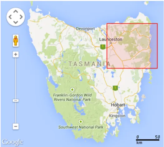
The main objective of this dissertation is to propose and to develop a computational field sim-ulation framework and environmental modelling application for swarm sensing application. Figure 3.1 depicts the Region of Interest (RoI) on which the field simulation will be based the South Esk region, Tasmania. To begin with, Table 3.1 presents summary attributes based on different sensor types to be deployed.

Fig. 3.1 Map of the state of Tasmania. The red rectangle (in the north-eastern corner of the map) is where Tasmanian’s South Esk region is located. (Image source: Google map)

(52)

26 Methodology

Attribute (a) Weather Station (b) Micro-sensors

Short Description A conventional weather station.

Micro-sensors each attached to a bee’s thorax (Figure 1.1).

Sensor Size Large Small (sub-millimetre)

Number of Sensors Small (N<10) Large (e.g., thousands)

Dynamics Static Mobile

Communication Wired Wireless

Energy Availability Unconstrained Constrained

Spatial Coverage Small (one location point) Large (various locations)

Table 3.1 Distinct types of sensor nodes to be deployed: (a) static weather station; and (b) mobile micro-sensors. Nindicates the number of sensor nodes.

to a base station), so that network connectivity and relay capability are not issues. Regular maintenance of the system will be conducted throughout the experiment to minimise data loss during system downtime. Since it is quite costly to set up a weather station, the number of deployments is usually low. This kind of sensor node only has a very small spatial coverage but could be configured to make high frequency measurements. Considering other factors such as power consumption and data storage, it is often set up in a way that data collection occurs only within a pre-defined time interval (5m, 30m, 1h, daily, etc) under the assumption of having unconstrained energy. For the purpose of this work, weather stations are categorised as the following entities: food and/or water sources, and bee hives (Table 3.2). Note that weather stations are placed at each of these entities/locations.

(53)

27

of this thesis, and is impractical to do so in this case (since it would require us to manipulate the insect flight paths). Since one of the main objectives of this dissertation is to propose a framework to simulate artificial bees, bee foraging flight path data is crucial. Therefore, this work will employ the modelled bee foraging flight paths data set which have been developed by the CSIRO’s Swarm Sensing team [80]. Further description of this component will be given in Section 3.1.3.

Sensor Type Item Deployment Strategy Number of Nodes Reading Frequency

Static Food source Manual 5 Hourly

Static Water source Manual 1 Hourly

Static Weather station Manual 4 Hourly

Static Hive Optimisation 5 Hourly

Mobile Insects Random

(foragers) 20

† Minute / Seconds †_{Number of nodes deployed each day, from a single hive.}

Table 3.2 This table shows the configuration of the field simulation to be deployed within the area of interest (South Esk region of Tasmania, see Figure 3.1).

Table 3.2 presents the configuration of our proposed hybrid environmental sensor net-works (ESN) field simulation at our Region of Interest (RoI). Based on the table, three types of stationary sensor nodes will be deployed for different purposes: (a) bee hive; (b) food and water sources for the bees; and (c) four extra weather stations located at the RoI’s map corner because the environmental modelling on the later stage is aninterpolationissue (instead of extrapolation). In addition, note that the table shows 20 bees will be created each day in each hive, which indicates that a total of 100 bees (5 hives×20 bees) will be generated every day.

Lastly, the research design being undertaken in this work is as follows:

1 Data collection.

High Resolution Environmental Modelling Application Using a Swarm of Sensor Nodes