Parallel Popular Crime Pattern Mining in Multidimensional Databases

(1)

Parallel Popular Crime Pattern Mining in

Multidimensional Databases

BVS. Varma#1_{, V. Valli Kumari}*2 #

Department of CSE, Sri Venkateswara Institute of Science & Information Technology Tadepalligudem, India

*

Department of CS&SE, AU College of Engineering, Andhra University Visakhapatnam, India

Abstract— Discovering interesting patterns like popular crime patterns from various geographical locations plays an important role in data mining and knowledge discovery process. The researchers have been extended the frequent patterns to different useful patterns such as sequential, cyclic, emerging, periodic and many other interesting patterns. PPCrime-growth algorithm has been introduced and it involves in mining popular crime patterns from various geographical locations. In performing, it captures the popularity of individual crimes among their peers or groups or crimes at their local site. PPCrime-tree will be constructed at every local node in the first phase which captures the essential data for the global mining process. In the next phase popular crime patterns will be extracted from PPCrime-tree in parallel. PPCrime-algorithm will work in parallel at each local site in order to reduce I/O cost and also Inter-process communication between nodes. Our method generates all

popular crime patterns in the final phase. The experiment

results show that our PPCrime-method is highly efficient in multidimensional databases.

Keywords—Popular patterns, crime patterns, geographical locations, inter-process communication, parallel algorithms, large databases.

I. INTRODUCTION

In today’s information era databases are essentially distributed. The organizations that operate in global markets need to perform data mining on either homogeneous or heterogeneous distributed data sources. The distributed data mining is the process of mining data that has been partitioned into one or more physically / geographically distributed compartments. Distributed data mining provides a framework for scalability into smaller subsets that require computational resources individually. In the literature, one of two statements is commonly accepts as how data is distributed across the sites either in homogeneously or heterogeneously. Both the viewpoints accept the conceptual view point that the data tables at each site are partitions of a single global table. In the homogeneous database, the global table is horizontally partitioned. The tables at each site are subsets of a global table and they have exactly the same attributes. In the heterogeneous database, the global table is vertically partitioned and each site contains a collection of columns that do not have same attributes. But, each tuple at each site is assumed to contain a unique identifier to facilitate matching. Distributed data mining addresses the impact of distribution of users, software’s and computational resources on the data mining process.

The size and high dimensionality of datasets normally available as input to the problem of pattern detection, makes it an ideal problem of solving multiple nodes in parallel. Memory and CPU speed limitations are the primary reasons that faced by a single node. So it is significant to design efficient parallel algorithm to do the job. The other reason comes from the fact that many transactional databases are already available in parallel databases or they are distributed at multiple nodes. The cost of bringing them all at one node or one computer for discovering various patterns can be prohibitively expensive.

However, tree based approaches have been adopted in most of the studies in this field on finding frequent patterns or other interesting patterns. In this paper we are proposing an efficient method to extract popular crime patterns using PPCrime-algorithm that obtains global popular crime patterns from various nodes. The rest of the paper is organized as follows. Section 2 discussed with related work and section 3 summarizes the problem definition and Section 4 describes PPCrime – method to find popular crime patterns in large databases. Our experimental analysis will be shown in section 5. Finally, we conclude the paper in section 6.

II. RELATED WORK

(2)

normally generated when support threshold is set to low, and most of them are found to be insignificant depending on the application or user constraint. As a result several techniques have been proposed recently to reduce the desire result set by some of the user interesting parameters such as closed [3] , kmost [4 ], maximum length [5] etc., are found to be useful in discovering frequent patterns of special interest among users. The other user interesting time interval parameter may be a regular pattern. Users may perhaps be interested on frequent patterns that occur at regular intervals. For example, a web site administrator to improve web page design may be interested in regularly visited web pages rather than on the heavily hit web pages for a specific period of time. The idea of maximal frequent itemset [6] was proposed in the year 1998, an itemset is maximal frequent if its support is frequent and it should not be a subset by any other frequent itemset. After the frequent patterns came into existence, numerous techniques have been introduced. These works are categorized into two main “categories”. First “category” mainly focuses on algorithmic efficiency i.e., to avoid the candidate generation-and-test approach of the Apriori algorithm, a tree-based algorithm called FP-growth was proposed to build an FP-tree to capture the contents of trans-actional database (TDB) so that frequent patterns can be mined recursively from the FP-tree with a restricted test-only approach. Techniques in the second “category” mainly focused on extending the notion of frequent patterns to other interesting or important existing patterns such as, episodes, maximal, clusters and closed item sets. However, the mining of these patterns are based on the support/frequency measure. While support/frequency is a useful metric, support-based frequent pattern mining may not be sufficient to discover. Crime pattern algorithms [7][8][9][10] used to derive crime patterns in order to assist public safety and security agencies in achieving their objective of deterring crime and promoting citizen’s safety. Leung C.K.S. et. al [11] [12] introduced popular pattern mining in transactions and in popular friends in social groups.

III.PROBLEM DEFINITION

In this section the basic definitions of the problem described.

Crime Transaction Popularity: Pop(X, ctj) of a pattern X

in crime transaction ctj measures the membership degree of

X in ctj. We compute the membership degree based on the

difference between the crime transaction length |ctj| and

pattern size |X|.

, | |

Long Crime Transaction Popularity: Pop(X, ctmaxCTL(X))

of a pattern X in crime transaction ctmaxCTL(X) measures the

membership degree of X in ctmaxCTL, where ctmaxCTL(x) is the

crime transaction having maximum length in DBX .

, max | | | |

Popularity: Pop(X) of a pattern X in the CTDB measures an aggregated membership degree of X in all crime transaction in the CTDB. It is defined as an average of all crime transaction popularities of X.

| | ∑ ∈ ,

Popular Crime: A user specified minimum popularity threshold min_pop is given, a crime X is considered popular if its popularity is atleast min_pop ( i.e Pop(X) ≥ minpop).

Popularity Pop(X): of a pattern X in the CTDB measures an aggregate membership degree of X in the CTDB. It is defined in terms of = ∑ _∈ | | as follows.

1

| | ,

∈

1

| | |

∈

| | |

| | | |

The proposed parallel mining technique to extract popular crime patterns from various geographical locations which was incorporated in multi-dimensional database. Performing popular crime pattern mining which captures the popularity of individual crimes among their peers or groups or crimes. The procedure works in parallel at each local site in order to reduce I/O cost and inter-process communication generates all popular crime patterns in the final phase.

IV.PARALLEL POPULAR CRIME MINING PROCESS

In this section we describe our proposed method called PPCrime approach to extract popular crime patterns in parallel at different locations. Different nodes indicate different locations, data where each node maintains resources like processor, memory, etc. Accumulate different databases from different resources and then divide this database into specified number of partitions with non-overlapping partitions in order to maintain data in multi dimensions at specified locations. Consider the instance crime database in the process of mining popular crime patterns in parallel.

Assume DB = {p1, p2, p3,……pn} be a number of partitions in parallel in a homogeneous distributed system. The database DB is alienated into equal number of n partitions like D1, D2, D3,……Dn, and each partition Di is

assigned to each individual partition pi. Let popularity of

Crime C is represented as Popi(C) in dbi and support count

of Crime C is represented as supi(C) and maximum

transaction length as maxTLi(C) in dbi. Pop(C), sup(C),

(3)

in database DB respectively. Let λ is user given minimum popularity threshold. To accumulate all regi(S) and supi(S)

from each partition to find global popularity Pop(C), global support count sup(S) and global maximal transaction length maxTL(C) respectively. Popular crime pattern C is mined which satisfies user given global popularity.

TABLE 1 CRIME DATABASES AT MULTIPLE LOCATIONS

In this process first databases are scanned once to get the count of every single item in every dimension. Finding popular 1-items are those whose calculations pass their corresponding threshold. In the second step, < x: support(x), maxCTL(x), Pop(x)> information is acquired at each domain items. The crimes with popularity which are less than given popularity are not eliminated as in frequent pattern mining instead their super pattern mining will takes place into considerations and checked whether they are popular crimes or not. Hence, super-pattern popularity checking is required to find the crimes that are popular or not. Now crimes appear in the pop-tree as long as their counts pass their corresponding threshold. Thus, a popular crime pattern which includes the whole taxonomy information about a crime is also interesting to the user. Finally, all popular crime patterns are generated by using recursively mining the pop-tree. This procedure is continued until all popular patterns for all single crimes are generated. The popular crimes which are generated at every dimension are accumulated at header node and then popular crimes are extracted based on user given popularity threshold globally.

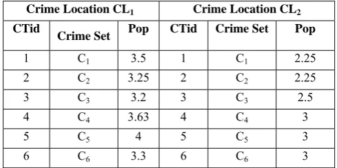
Consider the database Table 1, which indicates a list of crime data in two different locations. Table 2 represents popularity of each crime which is in two separate locations. Here, database is scanned once to get the count of every single crime in every single dimension. The popularity 1-dimensions are those whose counts pass their corresponding minimum popularity threshold. The minimum popularity threshold considered as 1.5 and the crimes whose count is less than minpop value are not eliminated as in frequent patterns instead their superset popularity checkup is considered. If its superset value exceeds minpop value then that crime will not be eliminated satisfies downward closure property. This process is repeated for n-dimensions.

Mining of popular crime patterns has been proposed by PPCrime-growth algorithm which consists of two key methods.

1. Construction of global PPCrime-tree

2. Mining of popular patterns from global PPCrime-tree Recall that, to mine popular crime patterns, the PPCrime-growth algorithm applies two key procedures: (i)

construction of a PPCrime-tree at local and (ii) mining of popular crime patterns from the PPCrime-tree. The PPCrime-growth finds popular crime patterns from the PPCrime-tree, in which each tree node captures its occurrence count, total transaction length, and maximum crime transaction length. The algorithm finds popular crime patterns by constructing the projected database for potential popular crime itemsets and recursively mining their

extensions. While constructing the conditional database from a projected database, perform a super-pattern popularity check for extensions of any unpopular crime, and delete the crime only when it fails the check. Such pruning technique was called as a lazy pruning. Recall that the PPCrime-growth recursively mines the projected databases of all items in Header table Table 4. Before constructing the projected database for a crime C in Header table, output the crime as a popular crime pattern if its popularity is at least minpop.

From Crime Location 1, calculate the popularities of each individual crime as follows

Pop(C1) = 18/4 – 1 = 3.5

Pop(C2) = 17/4 – 1 = 2.25

Pop(C3) = 21/5 – 1 = 3.2

Pop(C4) = 14/3 – 1 = 3.63

Pop(C5) = 10/2 – 1 = 4

Pop(C6) = 13/3 – 1 = 3.3

From Crime Location 2, calculate the popularities of each individual crime as follows

Pop(C1) = 13/4 – 1 = 2.25

Pop(C2) = 13/4 – 1 = 2.25

Pop(C3) = 14/4 – 1 = 2.5

Pop(C4) = 4/1 – 1 = 3

Pop(C5) = 7/2 – 1 = 2.5

Pop(C6) = 3/1 – 1 = 2

The popularities of each individual crimes of various crime locations are collected and stored at one place or in one tabe as a multidimensional database can be seen in Table 2.

TABLE 2 CRIME DATABASES AT MULTIPLE LOCATIONS WITH POPULARITY

Crime Location CL1 Crime Location CL2

CTid Crime Set CTid Crime Set

1 C1,C2, C3, C4, C5, C6 1 C3, C5, C6

2 C1,C2, C3, C4 2 C1,C2, C3, C4

3 C1,C2, C3, C5 3 C1,C2

4 C2, C3, C6 4 C1,C2, C3

5 C1, C3, C4, C6, 5 C1,C2, C3, C5

CTid

Crime Set Pop CTid Crime Set Pop

1 C1 3.5 1 C1 2.25

2 C2 3.25 2 C2 2.25

3 C3 3.2 3 C3 2.5

4 C4 3.63 4 C4 3

5 C5 4 5 C5 3

(4)

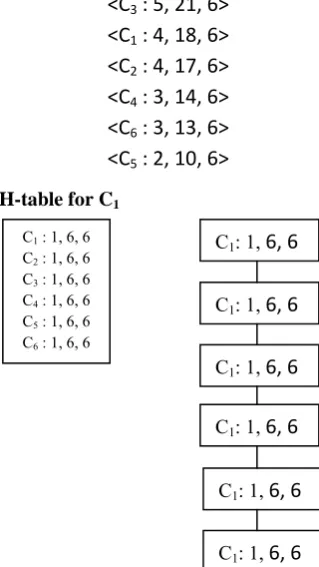
So here all crimes are popular. Now construct H table as follows <x:support(x), SumTL(x), maxTL(x)>

Arrange them in support descending order

H-table for C1

Fig 1. Length-1 PPCrime-tree Consider {C4}as projected database

(C4, C1) – 14/3 – 2 = 2.6

(C4, C2) – 10/2 – 2 = 3

(C4, C3) – 14/3 – 2 = 2.6

(C4, C5) – 6/1 – 2 = 3

(C4, C6) – 10/2 – 2 = 3

All length-2 crime itemsets are popular since all pop values are greater than minpop i.e., 1.5. Now consider the

projected database as {C3, C4}

{C1, C3, C4} ---- 14/3 – 3 = 1.6

{C2, C3, C4} ---- 10/2 – 3 = 2

{C5, C3, C4} ---- 6/1 – 3 = 3

{C6, C3, C4} ---- 10/2 – 3 = 2

The above length-3 crime itemsets are popular since all pop values are greater than minpop i.e., 1.5. Now consider the projected database as {C3, C4, C5}

{C1, C3, C4, C5} ---- 6/1 – 4 = 2

{C2, C3, C4, C5} ---- 6/1 – 4 = 2

{C6, C3, C4, C5} ---- 6/1 – 4 = 2

The above length-4 crime itemsets are also popular since all pop values are greater than minpop i.e., 1.5. Now consider the projected database as {C3, C4, C5, C6}

{C1, C3, C4, C5, C6} ---- 6/1 – 5 = 1

{C2, C3, C4, C5, C6} ---- 6/1 – 5 = 1

The above length-5 crime itemsets are not popular since all pop values are less than minpop i.e., 1.5. Fig 2 shows the local header table and local complete ppcrime-tree for Crime Location CL1.

H-table for C1 to C6

Fig 2. Complete PPCrime-tree for CL1

By using the above process mine the crime location CL2 to

find out the local header table and local ppcrime-tree. Fig 3 shows the local header table and local ppcrime-tree.

Header Table for C1 to C6

Fig 3. Complete PPCrime-tree CL2

C1: 3,14, 6

C2: 4,17, 6

C3: 2,10, 6 C3: 2, 7, 6

C4: 2,10, 6 C5: 1, 4, 6

C6: 1,3, 6

C5: 1,6, 6

C6: 1,6, 6

C3 : 5, 21, 6 C1 : 4, 18, 6 C2 : 4, 17, 6 C4 : 3, 14, 6 C6 : 3, 13, 6 C5 : 2, 10, 6

C1: 1,4, 6

C6: 1,4, 6

C4 1,4, 6

C3: 1,4, 6

C1: 1, 6, 6

C1 : 1, 6, 6 C2 : 1, 6, 6 C3 : 1, 6, 6 C4 : 1, 6, 6 C5 : 1, 6, 6 C6 : 1, 6, 6

C1 : 4, 13, 4

C2 : 4, 13, 4

C3 : 4, 14, 4

C4 : 1, 4, 4

C3: 1,4, 6 C1: 3, 9, 4

C2: 3, 9, 4

C3: 2, 7, 4

(5)

In crime location CL2, C5 and C6 are not popular since they

are less than minpop. The remaining crimes C1, C2, C3, C4

are popular.

TABLE 3. PPCRIME GLOBAL HEADER TABLE

Table 3 shows the global header table to find popular crime patterns from both the locations i.e., CL1 ad CL2. In fig 2

and fig 3 we find local popular crime patterns at each location. But our problem is to find global popular crime patterns. For this process global header table is useful to extract popular crime patterns. Table 4 shows the global popular crime patterns. The crime patterns (C4, C1), (C4,

C2), (C4, C3) are length-2 crimes which are popular in both

the locations CL1 ad CL2.

TABLE 4. LENGTH-2 POPULAR CRIME PATTERNS AT MULTIPLE LOCATIONS

In crime location CL1 (C4, C5) and (C4, C6) are popular

crimes but are not popular in CL2. These two patterns are

popular in local but are not in global. In this crime database the global maximum length crime patterns are (C4, C1), (C4,

C2), (C4, C3).

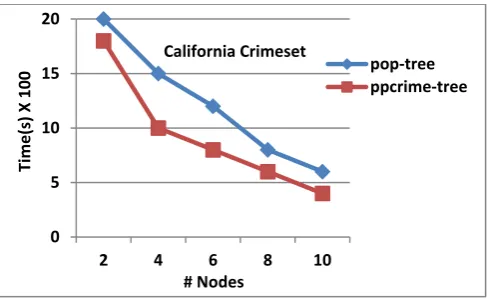
V. EXPERIMENT RESULTS

Fig 4. Execution time over 50K

Fig 5. Execution time over 100K

Our experimentation results are performed over crime dataset i.e., California crime dataset which is available as open source. Our algorithm PPCrime compared with the results of POP-tree which shows our algorithm is more efficient and fast in finding the popular crime patterns. All experiments are done in java on windows XP containing 2.7GHwith 2GB of main memory.

Fig 4 shows the execution time over California crime dataset on 50K records and 100K records in fig 5. The above two figures show our algorithm is more efficient than the existing pop-tree.

VI.CONCLUSION

Parallel computing is a necessary component in any large-scale data mining application. In large databases the performance of the parallel algorithms completely based on I/O cost and inter-process communication. In this paper we introduced a new mining method called PPCrime to mine popular crime patterns from different locations. This method works at each local node supporting to popularity and support counts which reduces inter process communication among the nodes and getting high degree of parallelism generates complete set of popular patterns at global. Experiments are conducted on crime data sets at various measures and also show that this method is efficient in terms of memory usage and execution.

REFERENCES

1. Agarwal, R., Imielinski, T., Swamy, A.N.: Mining Association Rules between sets of Items in Large Databases, ACM, SIGMOD Conference of Management of Data, pp. 207 – 216 (1993).

2. Han, J., Pei, J., Yin, Y.: Mining frequent patterns without candidate generation. In: ACM SIGMOD 2000, pp. 1–12 (2000).

3. Zaki, Mohammed J., and Ching-Jui Hsiao. Charm: an efficient algorithm for closed association rule mining, Vol. 10, Technical Report 99, 1999.

4. Minh, Q.T., Oyanagi, S., and Yamazaki K,” Mining the K-Most Interesting Frequent Patterns Sequentially” IDEAL 2006. LNCS, Springer, Heidelberg 2006, pp. 620 – 628.

5. Gouda Karam, and Mohammed Javeed Zaki. "Efficiently mining maximal frequent itemsets” Data Mining, 2001. ICDM 2001, Proceedings IEEE International Conference on. IEEE, 2001.

6. Chi Yun, Yirong Yang, Yi Xia and Richard R. Muntz.

“Cmtreeminer: Mining both closed and maximal frequent subtrees” Advances in Knowledge Discovery and Data Mining, Springer Berlin Heidelberg, 2004, pp. 63 – 73.

7. N. G. Khan, V. Bhaga, Effective data mining approach for crime-terrorpattern detection using clustering algorithm technique, 0

15 30 45 60

2 4 6 8

pop‐tree ppcrime‐tree

Time(sec)

# Nodes California Crimeset

0 5 10 15 20

2 4 6 8 10

pop‐tree ppcrime‐tree

# Nodes

Time

(s)

X

100

California Crimeset

Crime CL1 CL2 -- CLn Total

c1 pop1(c1) pop2(c1) -- popn(cn) i ( popi(c1))

c2 pop1(c2) pop2(c2) -- popn(cn) i (popi(c2))

--- --- _--- -- --- ---

cm pop1(cm) pop2(cm) -- popn(cm) i(popi(cm))

CTid Crime Set Pop CTid Crime Set Pop

1 C4, C1 2.6 1 C4, C1 2

2 C4, C2 3 2 C4, C2 2

3 C4, C3 2.6 3 C4, C3 2

4 C4, C5 3 4 - -

(6)

Engineering Research and Technology International Journal Vol 2 (4) (2013), pp. 2043–2048.

8. P. Phillips, I. Lee, Mining co-distribution patterns for large crime datasets, Expert Systems with Applications International Journal 39 (14) (2012) 11556–11563.

9. O. Isafiade, A. Bagula, Citisafe: Adaptive spatial pattern knowledge using fp-growth algorithm for crime situation recognition, in: Proc. IEEE International Conference on Ubiquitous Intelligence and Computing, IEEE, 2013, pp. 551–556.

10. D. Wang, W. Ding, H. Lo, T. Stepinski, J. Salazar, M. Morabito, Crime hotspot mapping using the crime related factors- a spatial data mining approach, Applied Intelligence Journal 39 (4) (2013) 772– 781.

11. Leung C.K.-S., Tanbeer S.K.: Mining Popular Patterns from Transactional Databases. Springer DaWak 2012, 291-302 (2012). 12. Leung C.K.-S., Tanbeer S.K.: Finding Popular Friends in Social